A Mixed-Fractal Model for Network Traffic

Abstract

In this short paper, we propose a new multi-fractal flow model, aiming to provide a possible explanation for the crossover phenomena that appear in the estimation of Hurst exponent for network traffic. It is shown that crossover occurs if the network flow consists of several components with different Hurst components. Our results indicate that this model might be useful in network traffic modeling and simulation.

1 Introduction

The fractal properties of network traffic were extensively studied in many literatures during the last decade. It is widely believed that the dynamic behavior of network flow under re-scaling needs to be carefully considered in performance analysis and control.

There are numerous explanations and models for the origins and appearances of fractality for network traffic; see e.g. [1]-[11] and the references therein. Under the multi-fractality assumption for Internet traffic, we propose a new flow model to explain the crossover phenomena found in the estimation of Hurst exponent [5], [11] (the crossover phenomenon is defined in the next section). Results indicate that this model help gain more insights into the actual network traffic dynamics. Moreover, we can use this model to better simulate network traffic in a simple way.

2 Self-Similarity and Multi-Fractality of Network Flow

In data networks, the traffic flow is often viewed a certain self-similar stochastic process $Y(k)$, which by definition satisfies [12]-[13]

$$Y(ak)\stackrel{{\scriptstyle d}}{{=}}a^{H}Y(k)$$ (1)

where $a>0$, and $\stackrel{{\scriptstyle d}}{{=}}$ denotes the equality of finite-dimensional distributions. $H>0$ is the so called Hurst exponent.

A self-similar process with stationary increments can then be defined by multiplexing the increments $X(k)=Y(k+1)-Y(k)$ over non-overlapping blocks of size $n$ as

$$X^{(n)}(k)=\sum_{j=0}^{n-1}X(kn-j),\indent k\in\mathbb{Z}$$ (2)

The aggregated process $X^{(n)}(k)$ is called a stationary self-similar $H$-SSS process with Hurst exponent $H$. It has finite-dimensional distributions similar to $X(k)$

$$X^{(n)}(k)\stackrel{{\scriptstyle d}}{{=}}n^{H}X(k),\indent n\in\mathbb{N}$$ (3)

There are various ways to study the stochastic properties of $X^{(n)}(k)$. [11] considers the cumulants of the aggregated series, which are defined as the Taylor coefficients of the cumulant-generating function

$$g(t)=\log\left(E(e^{tX})\right)=\sum_{m=1}^{\infty}\textrm{cum}_{m}(X)\frac{t^{m}}{m!}$$ (4)

with $\textrm{cum}_{m}(X)=g^{(m)}(0)$. In [14], [15], it is shown that the $m^{\textrm{th}}$ order cumulants of an aggregated $H$-sss process usually scales as

$$\textrm{cum}_{m}\left(X^{(n)}\right)\stackrel{{\scriptstyle\Delta}}{{=}}n^{mH(m)}\textrm{cum}_{m}\left(X(k)\right)$$ (5)

As pointed out in [11], Eq.(5) implies that for each $n,m\in\mathbb{N}$ the logarithm of the modulus of $\textrm{cum}_{m}\left(X^{(n)}(k)\right)$ scales linearly with $\log(n)$ with slope $mH(m)$ as

$$\log\left(\left|\textrm{cum}_{m}\left(X^{(n)}(k)\right)\right|\right)=mH(m)\log(n)+c(m)$$ (6)

The simplest form of $mH(m)$ is a linear function of $m$, i.e.

$$mH(m)=Am+B.$$ (7)

In [11], (7) is called linear-fractal model, where the coefficients $A$ and $B$ are directly estimated (interpolated) during the fittings to the cumulants.

A special case of the linear-fractal model is the uni-fractal model [6][11], which has the form

$$mH(m)=m+2(H-1)$$ (8)

where $H$ is the corresponding Hurst exponent.

[11] compared the linear-fractal model and the uni-fractal model using empirical network flow data. As shown in Fig.3 and Fig.4 of [11], although both models catch the main trends of the real data in the estimation of Hurst exponent., neither of them can perfectly match the so-called crossover phenomenon.

Fig.1 gives an illustration of the crossover phenomenon. In the current case the X-axis stands for $\log(n)$ and the Y-axis stands for $\log$ cumulant. The slope of the fitting curve crossovers from a small value to a notably larger value. Therefore the curve consists of three parts: a line segment with a gentler slope when $\log(n)$ is small, the intermediate transition part, and another line segment with a steeper slope when $\log(n)$ is large.

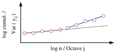
Figure 1: An illustration of the crossover phenomena of Hurst exponent which appears in the fractal model fitting to the cumulants and the logscale Diagram of wavelet based estimation.

The crossover phenomenon can also be observed in the wavelet-based Hurst coefficient estimation for network flow [5], [16]. As shown in [5], a self-similar process has the following power law

$$\textrm{Var}(y_{j})=C_{y}j^{(2H+1)}$$ (9)

where $C_{y}$ is a constant, $\textrm{octave}~{}j=\log_{2}(\textrm{scale})$, and $\textrm{Var}(y_{j})$ is a specially defined measuring variance on $\textrm{octave}~{}j$. Eq.(9) indicates that the logarithm of $\textrm{Var}(y_{j})$ scales linearly with $\log(j)$ with slope $(2H+1)$ as

$$\log\textrm{Var}(y_{j})=(2H+1)\log(j)+\log C_{y}$$ (10)

However, real flow data again exhibits the unexpected crossover phenomenon as illustrated in Fig.1, (in this case the X-axis stands for $\log(j)$ and the Y-axis stands for $\log$ cumulant). An example can be found in Fig.2.3 of [5].

There are numerous physical models for the origin of the self-similarities in network traffic flows, but few of them can explain the crossover phenomenon. This gap calls for a finer model that accounts for the crossover phenomenon, as it will not only enhance our understanding of the underlying mechanism of the network traffic, but may also lead to improvements of network performance.

3 A Mixed-Fractal Flow Model Yielding Crossover Phenomena

Our previous study [17] shows that the PCA eigen-spectrum of the mixed fBm signals with different Hurst exponents may yield bi-scaling/multi-scaling behavior. Inspired by that finding, we propose a mixed-fractal flow model, which reproduces the above crossover phenomena and sheds light on its origin.

We assume that the network flow process $W(k)$ is the sum of two independent self-similar processes $X_{1}(k)$ and $X_{2}(k)$ with different Hurst exponents $H_{1}$ and $H_{2}$, respectively:

$$W(k)=\lambda_{1}X_{1}(k)+\lambda_{1}X_{2}(k)$$ (11)

It is assumed that $\textrm{Var}\left\{X_{1}\right\}=\textrm{Var}\left\{X_{2}\right\}=1$ and thus $\lambda_{1}$ , $\lambda_{2}>0$ control the variance of the two components. Without loss of generality, we assume $H_{1}<H_{2}$.

Similarly to Eq. (2), we can define $Z^{(n)}(k)$ by multiplexing the increments $Z(k)=W(k+1)-W(k)$ over non-overlapping blocks of size $n\in\mathbb{N}$ as

$$Z^{(n)}(k)=\sum_{j=0}^{n-1}Z(kn-j),\indent k\in\mathbb{Z}$$ (12)

For the linear-fractal and uni-fratal models, we obtain by independence

$$\left|\textrm{cum}_{m}\left(Z^{(n)}(k)\right)\right|$$ (13)

$$= \left|\textrm{cum}_{m}\left(\lambda_{1}X_{1}^{(n)}(k)\right)\right|+\left|\textrm{cum}_{m}\left(\lambda_{2}X_{2}^{(n)}(k)\right)\right|$$

$$= c_{1}(m)n^{mH_{1}(m)}+c_{2}(m)n^{mH_{2}(m)}$$

$$= c_{1}(m)n^{\left[m+2(H_{1}-1)\right]}+c_{2}(m)n^{\left[m+2(H_{2}-1)\right]}$$

where $c_{1}(m)$ and $c_{2}(m)$ are partly determined by $\lambda_{1}$ and $\lambda_{2}$, respectively. In general, a larger $\lambda_{i}$ leads to a larger $c_{i}(m)$.

If $c_{1}(m)>c_{2}(m)$, there is a unique positive solution $n^{*}$ (not necessarily an integer) for the following equation in variable $n$

$$c_{1}(m)n^{\left[m+2(H_{1}-1)\right]}=c_{2}(m)n^{\left[m+2(H_{2}-1)\right]}$$ (14)

It is easy to find

$$\left|\textrm{cum}_{m}\left(Z^{(n)}(k)\right)\right|\approx\left\{\begin{array}[]{ll}c_{1}(m)n^{\left[m+2(H_{1}-1)\right]}\textrm{, for }n\ll n^{*}\\ c_{2}(m)n^{\left[m+2(H_{2}-1)\right]}\textrm{, for }n\gg n^{*}\end{array}\right.$$ (15)

Therefore, for each $m$, the logscale diagram of the $m^{\textrm{th}}$-order cumulants of $Z^{(n)}(k)$ consist of three parts: one line segment with slope $m+2(H_{1}-1)$ when $n$ is small, the intermediate transition part (which is often short), and another line segments with slope $m+2(H_{2}-1)$ when $n$ is large. This is precisely the crossover phenomenon. An example from simulation is given in Fig.2 below.

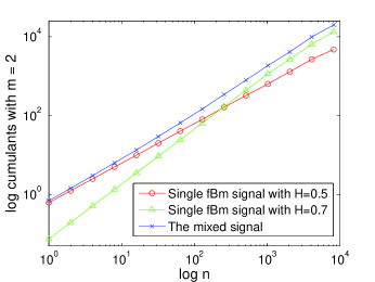
Figure 2: The crossover phenomena of Hurst exponent appears in the cumulant plot, where two self-similar processes with $H_{1}=0.5$ and $H_{2}=0.7$ are mixed with $\lambda_{1}=2\lambda_{2}$.

Similarly, for the wavelet model, we obtain by independence

$$\textrm{Var}(z_{j})=c_{3}j^{(2H_{1}+1)}+c_{4}j^{(2H_{2}+1)}$$ (16)

where $c_{3}$ and $c_{4}$ are partly determined by $\lambda_{1}$ and $\lambda_{2}$, respectively. In general, a larger $\lambda_{i}$ leads to a larger $c_{i}$.

If $c_{3}>c_{4}$, there exists a unique positive solution $j^{*}$ (not necessarily an integer) for the following equation in variable $j$

$$c_{3}j^{(2H_{1}+1)}=c_{4}j^{(2H_{2}+1)}$$ (17)

It is easy to find

$$\textrm{Var}(z_{j})\approx\left\{\begin{array}[]{ll}c_{3}j^{(2H_{1}+1)}\textrm{, for }j\ll j^{*}\\ c_{4}j^{(2H_{2}+1)}\textrm{, for }j\gg j^{*}\end{array}\right.$$ (18)

Therefore, the logscale diagram of $Z(k)$ consist of three parts: one line segment with slope $(2H_{1}+1)$ when $j$ is small, the intermediate transition part (which is often short), and another line segments with slope $(2H_{2}+1)$ when $j$ is large. An example from simulation is given in Fig.3.

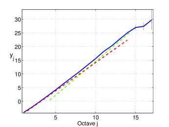
Figure 3: The crossover phenomena of Hurst exponent appears in the logscale Diagram of wavelet based estimation, where two self-similar processes with $H_{1}=0.5$ and $H_{2}=0.7$ are mixed with $\lambda_{1}=2\lambda_{2}$. We apply the Matlab code from [18] to obtain the logscale Diagram here.

In sum, we have shown that if the traffic flow process consists of two independent additive components with different Hurst exponents, we may observe the crossover phenomenon in the estimation of the Hurst exponents using cumulants or wavelets. It is not hard to see that this conclusion can be extended to the case with more than two components.

4 Concluding Remarks

In this section, we would like to index the following points:

First, it is interesting to find that the inconsistence of theoretical unique-fractal value of the Hurst exponent and the crossover phenomenon in real data may be resolved by a simple mixed-fractal model. Moreover, to simulate the mixed-fractal model, we can generate several processes with different Hurst exponents, using any of the existing methods for generating uni-fractal self-similar series, and then add them up. This is in accordance with the conclusion in [19] that we should multiplex multiple flow sources to generate more appropriate simulated traffic flows.

Secondly, most of the previous physical models for the origins of self-similarities in network traffic can be adopted to account for the co-existence of multiple heterogeneous self-similar components. For example, in the On/Off model [20], if it is further assumed that there exist two different values of the exponent parameters controlling the Pareto distributions of the ON-period/OFF-period of sources, then the aggregated flow will have two self-similar components with different Hurst exponents and thus exhibits crossover phenomenon. In general, in most complicated data networks, a channel is shared by many data sources (users) in an approximately independent and additive way. Due to the diversities of users and data transfer mechanisms, the inflow from different data sources might possess different Hurst components. This leads to the following conjecture: it is more likely to observe the crossover phenomenon in the traffic flows on backbone networks .

Thirdly, using either the cumulant or the wavelet based Hurst coefficient estimation, we can estimate the approximate varying range of the Hurst exponents. This work is very helpful, because a more appropriate and more accurate physical model often allows for a potential qualitative improvements on network performance [12], [21]-[22].

References

- [1] W. E. Leland, M. S. Taqqu, W. Willinger, and D. V. Wilson, “On the self-similar nature of Ethernet traffic (extended version),” IEEE/ACM Transactions on Networking, vol. 2, no. 1, pp. 1-5, Feb. 1994.
- [2] A. Erramilli, O. Narayan, and W. Willinger, “Experimental queueing analysis with long-range dependent packet traffic,” IEEE/ACM Transactions on Networking, vol. 4, no. 2, pp. 209-223, Apr. 1996.
- [3] M. S. Taqqu, V. Teverovsky, and W. Willinger, “Is network traffic selfsimilar or multifractal?” Fractals, vol. 5, no. 1, pp. 63-73, 1997.
- [4] P. Abry and D. Veitch, “Wavelet analysis of long-range dependent traffic,” IEEE Transactions on Information Theory, vol. 44, no. 1, pp. 2-15, Jan. 1998.
- [5] P. Abry, P. Flandrin, M. S. Taqqu, and D. Veitch, “Wavelets for the analysis, estimation and synthesis of scaling data,” in Self Similar Network Traffic Analysis and Performance Evaluation, K. Park and W. Willinger, eds., Wiley, 2000.
- [6] S. Molnár and G. Terdik, “A general fractal model of Internet traffic,” Proceedings of IEEE Conference on Local Computer Networks, Tampa, FL, pp. 492-499, Nov. 2001.
- [7] T. Karagiannis, M. Molle, M. Faloutsos, and A. Broido, “A nonstationary Poisson view of Internet traffic,” Proceedings of IEEE INFOCOM, Hong Kong, vol. 3, pp. 1558-1569, Mar. 2004.
- [8] Y. Chen, L. Li, Y. Zhang, and J. Hu, “Fluctuations and pseudo long range dependence in network flows: A non-stationary Poisson model,” Chinese Physics B, vol. 18, no. 4, pp. 1373-1379, 2009.
- [9] D. Veitch, N. Hohn, and P. Abry, “Multifractality in TCP/IP traffic: the case against,” Computer Networks, vol. 48, no. 3, pp. 293-313, June 2005.
- [10] W.-B. Gong, Y. Liu, V. Misra, and D. Towsley, “Self-similarity and long range dependence on the Internet: A second look at the evidence, origins and implications,” Computer Networks, vol. 48, no. 3, pp. 377-399, June 2005.
- [11] G. Terdik and T. Gyires, “Lévy flights and fractal modeling of Internet traffic,” IEEE/ACM Transactions on Networking, vol. 17, no. 1, pp. 120-129, Feb. 2009.
- [12] K. Park and W. Willinger, eds., Self-Similar Network Traffic and Performance Evaluation, John Wiley & Sons, Inc., 2000.
- [13] O. Sheluhin, S. Smolskiy, and A. Osin, Self-Similar Processes in Telecommunications, Wiley, 2007.
- [14] G. Samorodnitski and M. S. Taqqu, Stable Non-Gaussian Random Processes: Stochastic Models with Infinite Variance, Chapman & Hall/CRC, New York, 1994.
- [15] G. Terdik, Bilinear Stochastic Models and Related Problems of Nonlinear Time Series Analysis: A Frequency Domain Approach, Lecture Notes in Statistics, vol. 142, Springer Verlag, New York, 1999.
- [16] D. Veitch and P. Abry, “A wavelet based joint estimator of the parameters of long-range dependence,” IEEE Transactions on Information Theory, vol. 45, no. 3, pp. 878-897, April 1999.
- [17] L. Li, J. Hu, Y. Chen, and Y. Zhang, “PCA based Hurst exponent estimator for fBm signals under disturbances,” IEEE Transactions on Signal Processing, in press. (an online pre-print can be download from http://ieeexplore.ieee.org/xpl/tocpreprint.jsp?isnumber=4359509&punumber=78)
-
[18]
Matlab code for obtaining the Logscale Diagram is from
http://www.cubinlab.ee.unimelb.edu.au/~darryl/secondorder_code.html - [19] G. Horna, A. Kvalbeina, J. Blomskøld, and E. Nilsenb, “An empirical comparison of generators for self similar simulated traffic,” Performance Evaluation, vol. 64, no. 2, pp. 162-190, Feb. 2007.
- [20] W. Willinger, M. S. Taqqu, R. Sherman, D. V. Wilson, “Self-similarity through high-variability: statistical analysis of Ethernet LAN traffic at the source level,” IEEE/ACM Transactions on Networking, vol. 5, no. 1, pp. 71-86, Feb. 1997.
- [21] K. Park, T. Tuan, “Performance evaluation of multiple time scale TCP under self-similar traffic conditions,” ACM Transactions on Modeling and Computer, vol. 10, no. 2, pp. 152-177, April 2000.
- [22] G. He, Y. Gao, J. C. Hou, K. Park, “A case for exploiting self-similarity of network traffic in TCP congestion control,” Computer Networks, vol. 45, no. 6, pp. 743-766, Aug. 2004.