Reconstructing galaxy fundamental distributions and scaling relations from photometric redshift surveys. Applications to the SDSS early-type sample

Abstract

Noisy distance estimates associated with photometric rather than spectroscopic redshifts lead to a biased estimate of the luminosity distribution, and produce a correlated mis-estimate of the sizes. We consider a sample of early-type galaxies from the SDSS DR6 for which both spectroscopic and photometric information is available, and apply the generalization of the $V_{\rm max}$ method to correct for these biases. We show that our technique recovers the true redshift, magnitude and size distributions, as well as the true size-luminosity relation. We find that using only $10\%$ of the spectroscopic information randomly spaced in our catalog is sufficient for the reconstructions to be accurate within $\sim 3\%$, when the photometric redshift error is $\delta z\simeq 0.038$. We then address the problem of extending our method to deep redshift catalogs, where only photometric information is available. In addition to the specific applications outlined here, our technique impacts a broader range of studies, when at least one distance-dependent quantity is involved. It is particularly relevant for the next generation of surveys, some of which will only have photometric information.

1 Introduction

The redshift and luminosity distributions of galaxies, and galaxy scaling relations, such as the color-magnitude relation, the size-surface brightness relation, the luminosity-size relation or the Fundamental Plane, play a crucial role in constraining galaxy formation models. However, a bias will be intrinsically present in all these correlations if the transformation from observable to physical quantity involves one or more distance-dependent observables, due to noise in the distance estimate. Distances are only known approximately if photometric redshifts are available, but spectroscopic redshifts are not. This is already the case of many current surveys (e.g. SDSS, COMBO-17, MUSYC, COSMOS, CFHTLS), where the number of objects with photometric redshifts is more than an order of magnitude bigger than that of spectroscopic redshifts, and will be increasingly true of the next generations of deep multicolor wide-area photometric surveys (e.g. DES, LSST, SNAP, JDEM), which will increase the number of galaxies with multi-band photometry to a few billions.

Photometric information is essential and statistically more significant for studying cosmological evolution at a fraction of the cost of a full spectroscopic survey. Therefore, many efforts are currently devoted to improve photometric redshift estimations (see for example Feldmann et al. 2006; Carliles et al. 2008; Hildebrandt et al. 2008; Oyaizu et al. 2008a,b; Stabenau et al. 2008; Budavari 2009; Ilbert et al. 2009; Jouvel et al. 2009; Salvato et al. 2009), especially because accurate photometric redshifts are among the key requirements for precision weak lensing measurements (Banerji et al. 2008; Ma & Bernstein 2008; Mandelbaum et al. 2008). Well-understood photometric redshifts and errors are also vital in resolving redshift ambiguities where spectroscopy shows only a single spectral line (Lilly et al. 2007), and are especially crucial to dark energy science (Bernstein & Huterer 2009; Sun et al. 2009).

Hence, methods for recovering unbiased estimates of the redshift distribution (Padmanabhan et al. 2005; Sheth 2007; Lima et al. 2008), the luminosity function (Sheth 2007), and galaxy scaling relations (Rossi & Sheth 2008) from magnitude limited photometric redshift datasets are indeed necessary. In particular, in Rossi & Sheth (2008) we described two techniques which can handle this complication (i.e. a non-parametric deconvolution method and a maximum likelihood approach), and the extension of the $V_{\rm max}$ algorithm (Lucy 1974) was tested on a mock catalog. Here we apply the same method to the SDSS DR6, and investigate the bias present in the fundamental distributions and in the luminosity-size relation for early-type galaxies, which arises when computing these relations from photometric data. The technique is insensitive to the actual quality of photo-$z$ estimates, but it relies on the knowledge of the conditional probability $p(z_{\rm photo}|z_{\rm spectro})$. In essence, if photo-$z$ errors are at least known, our technique is applicable.

We have two main goals in this study. The first is to use a selected sample of early types from the SDSS DR6, for which both photo-$z$s and spectro-$z$s are known, and apply our deconvolution technique to derive the unbiased redshift, magnitude and size distributions, and the magnitude-size relation. We refer to this procedure as the “calibration” part. The second and more challenging goal is to use our calibration in order to infer information when spectroscopic data is poor or not available (i.e. deep redshift catalogs).

The outline of the paper is as follows. Section 2 describes the SDSS galaxy catalog used in this analysis, and highlights the criteria adopted for the early-type selection. Section 3 presents the reconstruction of the redshift, magnitude, size, and size-magnitude distributions from photometric data, for the early-type sample. A brief summary of the deconvolution method is provided – while we point out in an appendix the relation between our deconvolution procedure and a convolution-based approach –, the dependence of $p(z_{\rm photo}|z_{\rm spectro})$ on magnitude is also discussed, as well as other technical details. Section 4 deals with extending our technique when spectroscopic information is poor, or when only photometry is available. Some tests are performed on the early-type “calibration” catalog, and in particular it is found that, by using only $10\%$ of the spectroscopic information randomly spaced in redshift space, one can reconstruct accurately the galaxy fundamental distributions. Finally, Section 5 summarizes our findings, and indicate ongoing and future studies and applications.

Whenever necessary, we assume a spatially flat cosmological model with $(\Omega_{\rm M},\Omega_{\rm\Lambda},h)=(0.3,0.7,0.7)$, where $\Omega_{\rm M}$ and $\Omega_{\rm\Lambda}$ are the present day densities of matter and cosmological constant scaled to the critical density, and write the Hubble constant as $H_{0}=100~{}h~{}$ km s^-1 Mpc^-1.

2 The SDSS Early-Type Sample

The catalog we use is based on the Sloan Digital Sky Survey (SDSS) Data Release 6 (DR6, $http://www.sdss.org/$), available online through the Catalog Archive Server Jobs System (CasJobs). We adopt selection criteria suitable to early-type galaxies, as described in Bernardi et al. (2003). Specifically, from the DR6 galaxy photometric sample (PhotoObjAll in the Galaxy view, which contains primary objects that are classified as galaxies), we select objects according to these general criteria:

• Petrosian magnitudes in the range $14.50\leq m\leq 17.45$ for the $r$ band.

• Concentration index $R_{\rm petro,90}/R_{\rm petro,50}>2.5$ in the $i$ band.

• Likelihood of the de Vaucouleur’s model $>0.8$.

• Objects with both photometric and spectroscopic redshifts available.

No redshift or velocity dispersion cuts were made, although we tested the effect of a velocity dispersion cut ($\sigma>0$, so good S/N) and found no substantial difference. Our catalog contains 163,718 objects, and consists of model magnitudes, petrosian radii, de Vaucouleurs and exponential fit scale radii along with their corresponding axis ratios in the $r$ band, photometric and spectroscopic redshifts and their quoted errors.

Model magnitudes are obtained by measuring galaxy fluxes through equivalent apertures in all bands, and by fitting the exponential or de Vaucouleurs model of higher likelihood in the $r$ filter and applying it in the other bands, after convolution with a PSF in each band (for more details, see Blanton et al. 2003). The previous fitting procedures yield also the effective radii of the models and the axis ratio of the best fit model. In particular, the Petrosian ratio $R_{\rm P}$ at a radius $r$ from the center of an object is defined to be the ratio of the local surface brightness in an annulus at $r$ to the mean surface brightness within $r$, as described by Blanton et al. (2001) and by Yasuda et al. (2001). The Petrosian radius $r_{\rm P}$ is the radius at which $R_{\rm P}(r_{\rm P})$ equals some specified value $R_{\rm P,lim}$, set to $0.2$ in our case.

We select photometric redshifts from the SDSS Photoz table. This set of photometric redshifts has been obtained with the template fitting method, which simply compares the expected colors of a galaxy (derived from template spectral energy distributions) with those observed for an individual galaxy. The empirical templates of Coleman, Wu & Weedman (1980), extended with spectral synthesis models, are used. These templates were adjusted to fit the calibrations, as explained in Budavari et al. (2000). More detailed information about the photo-$z$ catalog used here is also provided in Csabai et al. (2003), and references therein. The main advantage of this technique in computing photo-$z$s is a broader redshift range coverage for all types of galaxies, and the additional information like spectral type, K-correction and absolute magnitudes. However, its accuracy is severely limited by the lack of perfect spectral energy distribution (SED) models. In fact, the quality of photometric redshift estimation of faint objects (or with large photometric errors) is weak. More generally, the standard scenario for template fitting is to take a small number of spectral templates and choose the best fit by optimizing the likelihood of the fit as a function of redshift, type and luminosity. Variations of this approach have been developed in the last few decades. For example, in the recent SDSS DR7 photometric redshifts are obtained with a hybrid method, namely a combination of the template fitting procedure and of a technique which compares the observed colors of galaxies to a reference set that has both colors and spectroscopic redshifts observed.

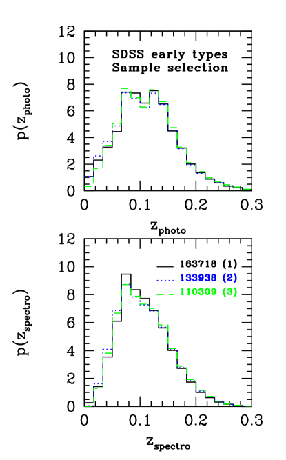
Figure 1: Photometric and spectroscopic SDSS redshift distributions for the early-type sample: effect of the selection criteria. Solid lines represent the redshift distributions of the sample considered in this study (Sample 1). Dotted lines are the result of using only spectra of good quality (Sample 2). Dashed lines denote a more sophisticated selection process, as explained in the main text (Sample 3).

Table 1: Median spectroscopic and photometric redshifts, corresponding median absolute deviations (MAD), standard normalized median absolute deviations (NMAD) and dispersions for the three early-type samples illustrated in Figure 1.

	SAMPLE 1	SAMPLE 2	SAMPLE 3
median $z_{\rm spectro}$	0.1021	0.1021	0.1040
median $z_{\rm photo}$	0.1107	0.1093	0.1131
MAD $z_{\rm spectro}$	0.0307	0.0328	0.0327
MAD $z_{\rm photo}$	0.0348	0.0361	0.0358
NMAD	0.0172	0.0173	0.0154
$\sigma_{\rm\Delta z/(1+z_{\rm spectro})}$	0.0340	0.0263	0.0219

We finally cross-correlate the photometric information with the SDSS DR6 spectroscopic sample (SpecObjAll), and select only those photometric objects for which spectroscopic information is also available. The spectroscopic pipeline (spectro1d) assigns a final redshift to each object spectrum by choosing the emission or cross-correlation redshift with the highest likelihood and stores this as $z$ in the specObj table. In addition to spectral classification based on measured lines, galaxies are classified by a Principal Component Analysis (PCA), using cross correlation with eigentemplates constructed from the SDSS spectroscopic data. In the selection of our sample we use only photometric criteria, but more robust constraints can be applied in order to reduce galaxy-type errors, and their effect is illustrated in Figure 1. In both panels, solid lines represent the redshift distributions of the calibration sample used in this study (Sample 1). However, if in addition we require spectra of good quality or without masked regions (SDSS warning flag for spectra of low quality set to zero), then the number of galaxies drops to $133,938$ (dotted lines in Figure 1, Sample 2). Finally, if we consider only spectra with PCA classification numbers $a<-0.1$, typical of early-type galaxy spectra (Connolly & Szalay 1999), we find $110,309$ objects (dashed lines in Figure 1, Sample 3). For all these samples, we provide in Table 1 the median spectroscopic and photometric redshifts, their corresponding median absolute deviations (MAD), the standard normalized median absolute deviation (NMAD) defined as in Hoaglin et al. (1983) by $1.48\times median[|\Delta z|/(1+z_{\rm spectro})]$, and the dispersion $\sigma_{\rm\Delta z/(1+z_{\rm spectro})}$, where $\Delta z=z_{\rm spectro}-z_{\rm photo}$.

In our study we consider the sample obtained with the photometric-only selection process (Sample 1). This is because our second goal is to rely on this “calibration” subset to infer information when only photometry is available.

More sophisticated criteria for obtaining a well-controlled sample of early-type galaxies are presented in Park and Choi (2005) who used color, color-gradient, and concentration index to classify galaxies into early and late types with reliability and completeness exceeding $90\%$. See also Hyde & Bernardi (2009), where problems like contamination by later-type galaxies and systematic effects due to the use of Petrosian quantities are addressed in detail. However, since we are not attempting to make a precision measurement of scaling relations, but rather our main goal is to show how to correct for photo-$z$ biases, more robust selection criteria do not affect the nature of the problems investigated in this study.

3 Deconvolutions from photometric data

In this section we apply our reconstruction technique based on the generalization of the $V_{\rm max}$ method (Sheth 2007; Rossi & Sheth 2008) and briefly summarized here to the redshift, magnitude and size distributions, and to the size-luminosity relation of the early-type sample. A new deconvolution code named DeFaST (acronym for Deconvolution Fast, with the convention of using capital letters for consonants), which performs a fast integral deconvolution, has been developed for this study. Lucy’s (1974) iterative scheme is implemented, in one or two dimensions. Appropriate variations have been carried out in order to handle correctly different choices of the conditional probability functions. In particular, for the SDSS early-type sample the conditional distributions are measured directly from the data and then used in the deconvolution algorithm. Splines fits to the pdf’s are performed in those cases. For technical details we refer the reader to a trial version of the one-dimensional software, freely available for download online at the web address $http://www.physics.upenn.edu/\sim grossi/research/software.htm$.

3.1 Extended $V_{\rm max}$ method as a non-parametric deconvolution-like technique

The $V_{\rm max}$ method, originally devised by Schmidt (1968), is a way of testing the uniformity of spatial distributions. In particular, if $V$ is the comoving volume between an object in a flux-limited catalog at redshift $z$ and the observer located at $z=0$, and $V_{\rm max}$ is the corresponding total survey volume over which the same object could have been seen at $z_{\rm max}$, then clearly the ratio $V/V_{\rm max}$ is a measure of the position of the source. Therefore, if a distribution is uniform then the average value over all the objects in the catalog, $\langle V/V_{\rm max}\rangle$, must be 0.5. The $V_{\rm max}$ method allows one to correct for selection effects present in magnitude-limited datasets, where fainter objects are seen only at closer distances. In fact, in order to properly estimate for example the luminosity function one must sum over all the objects in the catalog and weight each source separately by the inverse of $V_{\rm max}$ (or the inverse of $V_{\rm max}-V_{\rm min}$ if the catalog is limited at both ends). This is the basis of the procedure developed by Schmidt (1968).

Generalizations of this method to include distance errors have been carried out in Sheth (2007) for the luminosity function (1D case), and in Rossi & Sheth (2008) for galaxy scaling relations (2D case, or full $n$-dimensional manifold). To summarize, in a flux-limited survey the quantities affected by the photometric redshift errors are the intrinsic luminosity distribution rather than the luminosity function itself (which differs from the previous one by the inclusion of a $1/V_{\rm max}$ weighting), and the intrinsic joint distribution of luminosities and sizes – or in general the joint distribution of two (or more) observables affected by the same distance errors. However, in a real experiment one measures their noisy counterparts. Therefore it is necessary to reconstruct the intrinsic distributions first, before applying the $V_{\rm max}$ prescription. This is achieved by recognizing the deconvolution nature of this class of problems, hence an iterative algorithm is suitable for the reconstructions.

In fact, adopting Lucy’s (1974) formalism, the general $n$-dimensional problem is that of estimating the frequency distribution $\Psi({{\mbox{\boldmath$\xi$}}})$ of the intrinsic $n$-dimensional vector $\xi$ when the available observed measures, denoted by the vector $x$, are a finite sample drawn from an infinite population characterized by

$$\Phi({{\mbox{\boldmath$x$}}})=\int\Psi({{\mbox{\boldmath$\xi$}}})~{}p({{\mbox{\boldmath$x$}}}|{{\mbox{\boldmath$\xi$}}})~{}{\rm d}{{\mbox{\boldmath$\xi$}}},$$ (1)

where $\Phi({{\mbox{\boldmath$x$}}})$ is the data function accessible to measurements and $p({{\mbox{\boldmath$x$}}}|{{\mbox{\boldmath$\xi$}}})$ is the conditional probability of estimating $x$ when the true value is $\xi$. The iterative procedure to invert the previous expression is

$$\Psi^{\rm r+1}({{\mbox{\boldmath$\xi$}}})=\Psi^{\rm r}({{\mbox{\boldmath$\xi$}}})\int{\rm d}{{\mbox{\boldmath$x$}}}~{}\frac{\tilde{\Phi}({{\mbox{\boldmath$x$}}})}{\Phi^{r}({{\mbox{\boldmath$x$}}})}~{}p({{\mbox{\boldmath$x$}}}|{{\mbox{\boldmath$\xi$}}}),$$ (2)

where

$$\Phi^{\rm r}({{\mbox{\boldmath$x$}}})=\int{\rm d}{{\mbox{\boldmath$\xi$}}}~{}\Psi^{\rm r}({{\mbox{\boldmath$\xi$}}})~{}p({{\mbox{\boldmath$x$}}}|{{\mbox{\boldmath$\xi$}}}).$$ (3)

The index $r$ indicates the $r$th iteration in the sequence of estimates, and $\tilde{\Phi}$ is an approximation to $\Phi$ obtained from the observed sample. The starting value $\Psi^{0}({\mbox{\boldmath$\xi$}})$, which initializes the iteration, should be a smooth, non-negative function having the same integrated density as the observed distribution. In our deconvolution procedure, we always use the observed histograms (i.e. photo-$z$ derived distributions) as convenient starting guesses.

Clearly, the outlined formalism is readily applicable to the size-luminosity correlation if we interpret $x$ as the 2D vector of the estimated absolute magnitudes and sizes, and $\xi$ as the vector of the corresponding true (or intrinsic) quantities. Similarly for the redshift, magnitude and size distributions, where now vectors simply reduce to scalar quantities (1D case).

3.2 Redshift distribution

Following Rossi & Sheth (2008), we indicate with $\zeta$ and $z$ the photometric and spectroscopic redshifts, respectively. As argued before, the problem of estimating the intrinsic redshift distribution $N(z)$ – number of objects which lie at redshift $z$ – is best thought of as a deconvolution problem, and if $p(\zeta|z)$ is the probability of estimating the redshift as $\zeta$ when the true value is $z$, then the distribution of estimated redshifts is ${\cal N}(\zeta)=\int N(z)~{}p(\zeta|z)~{}{\rm d}z$. Note that this is just a particular 1D case of equation (1), where ${{\mbox{\boldmath$\xi$}}}\rightarrow z$, ${{\mbox{\boldmath$x$}}}\rightarrow\zeta$, $\Phi\rightarrow{\cal N}$ and $\Psi\rightarrow N$. If $p(\zeta|z)$ is known and ${\cal N}(\zeta)$ is measured, then the previous relation is a Fredholm equation of the first kind, easily solvable with a one-dimensional inversion algorithm. Before showing the reconstructed intrinsic redshift distribution, we focus our attention on the conditional probability $p(\zeta|z)$. In reality, this distribution does depend weakly on apparent magnitude. To illustrate the effect, we split our early-type sample in three intervals of apparent magnitudes, approximately spaced in bins of $1.5$ magnitude width, i.e. $13.81\leq m<15.31$ (solid lines in Figure 2), $15.31\leq m<16.81$ (dotted lines in Figure 2), $16.81\leq m<18.27$ (dashed lines in Figure 2). In the left panel of Figure 2, contours show levels which are $1/2^{n}$ times the height of the maximum value of the density of sources, with $n$ running from $1$ to $5$, for the three magnitude bins. In the same figure, the right panel shows an example of $p(\zeta|z,m)$ for each of the three bins in magnitude and a spectroscopic redshift bin centered on $z=0.0572$.

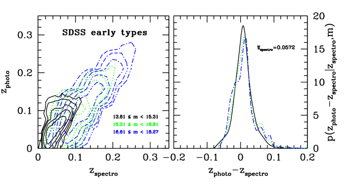
Figure 2: Apparent magnitude dependence of the conditional probability $p(\zeta|z)$. [Left panel] Contours show levels which are $1/2^{n}$ times the height of the maximum value of the density of sources, with $n$ running from $1$ to $5$, for the three magnitude bins specified in the figure. [Right panel] Example of $p(\zeta-z|z,m)$ for $z=0.0572$ and for the three previous bins in magnitude.

Neglecting this small dependence of magnitude does not affect the reconstruction of the intrinsic redshift distribution significantly. Results are shown in Figure 3, where in the left panel we compare $\zeta$ and $z$, whereas in the right panel we show the photometric or observed redshift distribution (dotted line), the spectroscopic or intrinsic distribution (solid line) and its reconstruction after a few iterations (dashed line), obtained by applying the one-dimensional deconvolution algorithm based on the Lucy’s (1974) inversion technique. The error distributions used in the reconstruction are inferred directly from the SDSS early-type data. The median redshift of the spectroscopic sample is 0.1021 (see Table 1), while the median redshift of the deconvolved photo-$z$ distribution is 0.1002. This value is calculated as follows. We find the bin which divides the reconstructed spectroscopic distribution in two roughly equal area parts. Within that bin, we then interpolate with splines and provide the exact value of z for which the area of the reconstructed distribution is split into two equal parts.

Accurately characterizing $p(\zeta|z)$ is necessary for a reliable deconvolution. After testing different methods, we have achieved good results using cubic splines and found that simple Gaussian fits provide unsatisfactory mapping of the conditional distributions (see also Section 4.3).

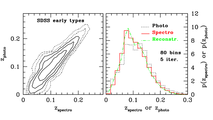
Figure 3: [Left panel] Distribution of spectroscopic and photometric redshifts in our SDSS early-type catalog. Contours as in Figure 2. [Right panel] Observed, intrinsic and reconstructed redshift distributions. The dotted histogram was used as a starting guess for the one-dimensional deconvolution algorithm. Convergence is achieved after a few iterations.

3.3 Magnitude distribution

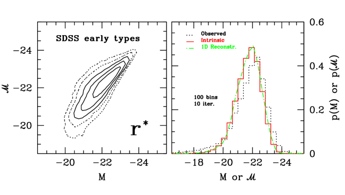
Figure 4: [Left] Distributions of intrinsic and estimated absolute magnitudes in the SDSS early-type catalog, which result from the differences between spectroscopic and photometric redshifts shown in the previous figure. [Right] One-dimensional reconstruction of the intrinsic absolute magnitude distribution from the distribution of estimated redshifts. Dotted histogram shows the observed absolute magnitude distribution, used as a starting guess. Jagged line is the reconstructed intrinsic distribution, after $10$ iterations.

The previously outlined dependence of $p(\zeta|z)$ on apparent magnitude suggests that one should expect, similarly, a redshift dependence in the corresponding magnitude conditional distributions. Therefore, it may appear difficult to characterize and measure the appropriate conditional probabilities, and apply the one-dimensional deconvolution algorithm to reconstruct the magnitude distribution. However the problem is simpler, as we show with the following algebra. Let $M$ denote the true absolute magnitude and $\cal M$ that estimated using $\zeta$ rather than $z$. Use $D_{\rm L}(z)$ to denote the luminosity distance, and $\phi(M)$ to indicate the number density of galaxies with absolute magnitudes $M$. Evolution is neglected. Let $V_{\rm max}$ denote the largest comoving volume out of which an object of absolute magnitude $M$ can be seen, and $V_{\rm min}$ the analogous if the catalog is also limited at the lower end. The (true) number of galaxies with absolute magnitude $M$ (i.e. the intrinsic luminosity distribution) is:

$$N(M)=\phi(M)[V_{\rm max}(M)-V_{\rm min}(M)],$$ (4)

and the total number of objects with estimated absolute magnitudes $\cal M$ is:

$${\cal N}(\cal M) = \int{\rm d}M~{}\phi(M)~{}\Theta[V_{\rm max}(M),V_{\rm min}(M),M,{\cal M}]$$

$$= \int{\rm d}M~{}N(M)~{}\frac{\Theta[V_{\rm max}(M),V_{\rm min}(M),M,{\cal M}]}{[V_{\rm max}(M)-V_{\rm min}(M)]},$$

where

$$\Theta=\int_{D_{\rm L}(V_{\rm min})}^{D_{\rm L}(V_{\rm max})}{\rm d}D_{\rm L}~{}\frac{{\rm d}V_{\rm com}}{{\rm d}D_{\rm L}}~{}p(M-{\cal M}|M,D_{\rm L}).$$ (6)

Note that since $V_{\rm max}$ and $V_{\rm min}$ are known functions of $M$, $\Theta$ itself is just a complicated function of $M$ and ${\cal M}$. Dividing (6) by $[V_{\rm max}(M)-V_{\rm min}(M)]$ yields:

$$\frac{\Theta}{[V_{\rm max}-V_{\rm min}]} = \int{\rm d}D_{\rm L}~{}\frac{{\rm d}V_{\rm com}/{\rm d}D_{\rm L}}{[V_{\rm max}-V_{\rm min}]}~{}p(M-{\cal M}|M,D_{\rm L})$$ (7)

$$= \int{\rm d}D_{\rm L}~{}p(D_{\rm L})~{}p(M-{\cal M}|M,D_{\rm L})$$

$$= p(M-{\cal M}|M)\equiv p({\cal M}|M).$$

Therefore, equation (5) becomes a simple one-dimensional deconvolution, namely:

$${\cal N}({\cal M})=\int N(M)~{}p({\cal M}|M)~{}{\rm d}M.$$ (8)

The above expression (8) is again another particular 1D case of (1), where now ${{\mbox{\boldmath$\xi$}}}\rightarrow M$, ${{\mbox{\boldmath$x$}}}\rightarrow{\cal M}$, $\Phi\rightarrow{\cal N}$ and $\Psi\rightarrow N$. Hence, by measuring the conditional probability $p({\cal M}|M)$ from the catalog, it is possible to apply directly the one-dimensional deconvolution algorithm – as in the previous section. Note that this conclusion is particularly relevant when attempting to reconstruct the luminosity function from photometric data. Results of this applications are shown in Figure 4, where the left panel compares ${\cal M}$ and $M$, while the right panel shows the one-dimensional reconstruction after $10$ iterations (jagged line) of the intrinsic distribution of absolute magnitudes (solid histogram). The observed distribution of $\cal M$ (dotted histogram) was used as a convenient starting guess in the deconvolution algorithm. We use model magnitudes in the r band, corrected for reddening and extinction, and assume a standard cosmology in the conversion from apparent to absolute magnitudes – but we neglect evolution and K-corrections. In particular, while K-corrections are necessary to properly characterize the absolute magnitude distribution, in this paper we do not apply them to our de-reddened model magnitudes because the only purpose of our work is to describe a deconvolution technique, which is independent of those corrections.

3.4 Size distribution

Figure 5: [Upper left] Distribution of seeing-corrected effective angular sizes of galaxies in our early-type SDSS sample. [Upper right] Corresponding distribution of axis ratios $b/a$. [Lower left] Effective angular sizes $r_{\rm deV}$ as a function of the axis ratio $b/a$. [Lower right] Distribution of effective circular radii $r_{\rm 0,deV}$, as defined in the main text.

As for the magnitude distribution, it is possible to reconstruct the intrinsic distribution of sizes with a one-dimensional deconvolution algorithm (for more details, see also Section 3.3 in Rossi & Sheth 2008). In what follows, we use $R$ to denote $\log_{\rm 10}$ of the physical size, and $\cal R$ to denote the estimated size based on the photometric redshift $\zeta$. We apply one correction to convert the (seeing-corrected) effective angular radii, $r_{\rm deV}$, output by the SDSS pipeline to physical radii. Following Bernardi et al. (2003), we define the equivalent circular effective radius $r_{\rm 0}=\sqrt{b/a}~{}r_{\rm deV}$, where $b/a$ is the corresponding axis ratio of the de Vaucouleurs radius. Then $R=\log_{\rm 10}[r_{\rm 0}D_{\rm L}(z)/(1+z)^{2}]$, and similarly ${\cal R}=\log_{\rm 10}[r_{\rm 0}D_{\rm L}(\zeta)/(1+\zeta)^{2}]$. We do not apply a second correction, analogous to the K-correction we would ideally have applied to the magnitude of each galaxy, to account for the fact that galaxies appear slightly larger in the bluer bands (i.e. Hyde & Bernardi 2009). Figure 5 shows the distribution of seeing-corrected effective angular sizes of galaxies in our SDSS early-type sample (upper left panel), the corresponding distribution of axis ratios $b/a$ (upper right panel), the effective angular sizes $r_{\rm deV}$ as a function of axis ratio $b/a$ (lower left panel), and the distribution of equivalent circular effective radii $r_{\rm 0,deV}$ (lower right panel).

In analogy with the magnitude case, we think of ${\cal N}({\cal R})$, the number of observed objects with estimated ${\cal R}$, as being a convolution of the true number of objects with size $R$, $N(R)$, with the probability that an object with size $R$ is thought to have size ${\cal R}$. We measure $p({\cal R}|R)$ directly from the catalog and run the one-dimensional deconvolution algorithm, the result of which is presented in Figure 6. The left panel compares ${\cal R}$ and $R$, and the right panel shows the one-dimensional reconstruction (jagged line). The intrinsic distribution of physical sizes (solid line) is recovered after a few iterations, when the observed distribution of $\cal M$ (dotted line) is used as a convenient starting guess in the inversion algorithm. Note that although the difference between the intrinsic and the observed distribution is small, this departure will suffice to bias the size-luminosity relation – as we show next.

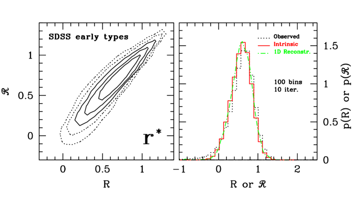
Figure 6: [Left panel] Distributions of intrinsic and estimated physical sizes in the SDSS early-type catalog. [Right panel] One-dimensional reconstruction of the intrinsic size distribution from the distribution of estimated redshifts. Dotted histogram shows the observed size distribution, used as a starting guess. Jagged line shows the reconstructed intrinsic distribution after $10$ iterations. Line styles same as Figure 4.

3.5 Size-magnitude correlation

Photometric redshift errors broaden both the magnitude and size distributions, as evident from Figures 4 and 6, but changes to the estimated absolute magnitudes and sizes are clearly not independent. These correlated changes have an important effect on the size-luminosity relation, even when the broadening of one of the two distributions is not severe. This is the case of our SDSS sample, where the size distribution (Figure 6) is not severely biased, but the size-luminosity relation is still biased. In fact, in our SDSS catalog $\langle{\cal R}|{\cal M}\rangle\propto-0.226$, whereas $\langle R|M\rangle\propto-0.257$, as shown in Figure 7.

Reconstructing an unbiased estimate of size and luminosity from photometric data is also best thought of as a non-parametric two-dimensional deconvolution (again, see Rossi & Sheth 2008), and application of the extended $V_{\rm max}$ 2D algorithm to the SDSS early-type sample is presented in Figure 7, where it is shown that the use of photo-$z$s introduces a bias in the size-luminosity relation (shallower slope in panel on left). Contours and solid lines indicate respectively the ${\cal R}-{\cal M}$ relation associated with photo-$z$ (left), and the expected intrinsic $R-M$ relation (right). Squares in left panel show the binned starting guess for the two-dimensional deconvolution algorithm (obtained from photometric information), triangles in right panel show the result after $7$ iterations and circles are the expected binned intrinsic relation, obtained from spectroscopic information. Convergence to the true solution is clearly seen.

As pointed out in Hyde & Bernardi (2009), most of the scaling relations for early types show evidence for curvature. In this respect, our technique also accounts for it, as we reconstruct intrinsic relations within each bin, without performing any fits.

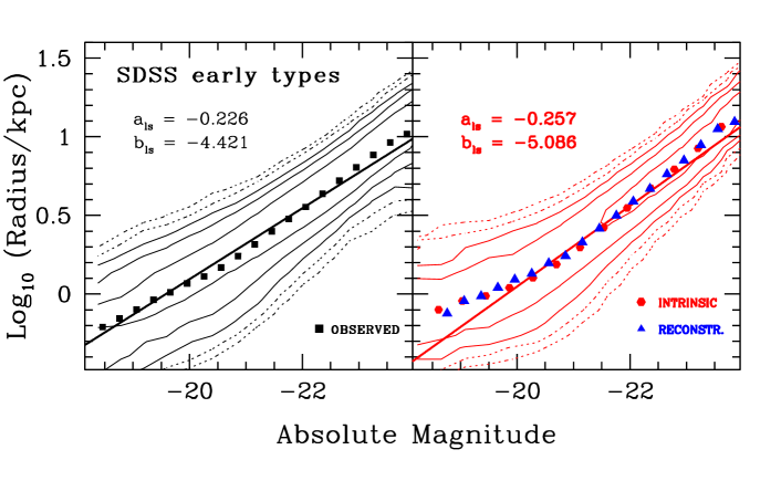
Figure 7: Effect of photo-$z$s on the size-luminosity correlation in our SDSS early-type catalog. In the left panel, contours and solid line show the ${\cal R}-{\cal M}$ relation associated with photo-$z$s, whereas the right panel shows the intrinsic $R-M$ relation. Note the bias (shallower slope in panel on left) which results from the fact that the photo-$z$ distance error moves points down and left or up and right on this plot. Squares in left panel show the binned starting guess for the 2D deconvolution algorithm, triangles in right panel show the result of reconstruction after 7 iterations. Circles are the expected binned intrinsic relation, obtained from spectroscopic information. Convergence to the true solution is clearly seen.

4 EXTENSIONS TO DEEP REDSHIFT CATALOGS

4.1 Challenges

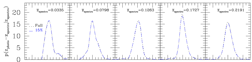
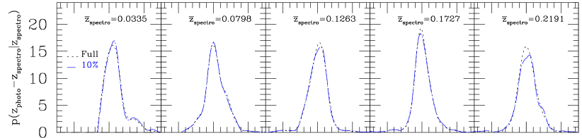
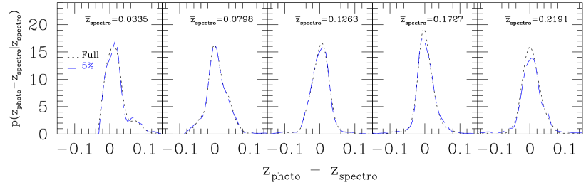
Figure 8: Measurements of the conditional probabilities $p(\zeta-z|z)$’s for five different spectroscopic redshift bins, as indicated in the panels. Dotted lines are spline fits to the pdf’s when the full spectroscopic information is used; long-dashed lines are spline fits when only $15\%$ [upper panel], $10\%$ [middle panel], or $5\%$ [lower panel] of the spectral information is used from the original early-type catalog.

If we derive galaxy fundamental distributions and scaling relations using only photometry, a bias will be intrinsically present – as was shown in the previous section. With our deconvolution procedure we can account and correct for it. However, our $V_{\rm max}$ reconstruction method assumes that the distribution of photo-$z$ errors is known accurately. This means that spectroscopic redshifts are available for a subset of the data, as it happens with our SDSS “calibration” sample. Suppose now that we only have limited spectroscopic data available. Can we still correct for the bias in a reliable way, using the information contained in the spectroscopic “calibration” set?

There are essentially two nontrivial issues to this end. As we pointed out in Rossi & Sheth (2008), one concern is as to whether or not the number of spectra which must be taken to specify the error distribution reliably is sufficient to also provide a reliable spectroscopic estimate of these fundamental distributions and scaling relations. In this case, the basis for deciding that it is worth reconstructing these relations from photo-$z$ data is not clear. However, as long as the spectroscopic sample spans the entire range of photometric observables, we show in the next subsection that a detailed knowledge of the photo-$z$ error distribution (Figure 8) can be inferred with only $10\%$ of randomly spaced spectra in redshift space. This rather conservative choice will guarantee an accurate reconstruction of the intrinsic relations. Cross-correlations with other surveys may also provide enough reliable information to specify $p(\zeta|z)$ accurately.

The second problem is more challenging. If the spectra are not simply a random subset of the magnitude limited photometric sample, then it may be difficult to quantify and so correct for the selection effects associated with the spectroscopic subset. In particular, if the spectroscopic sub-sample does not span the entire range of photometric observables, it is problematic to perform the reconstruction. However, in this situation one may rely on photo-$z$ error estimates for the range where spectral information is missing, and still apply the deconvolution procedure. We investigate this idea further in the second subsection, and discuss its applicability and limitations.

4.2 How many spectra?

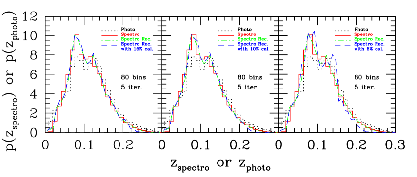
Figure 9: Reconstructions of the intrinsic redshift distribution (long-dashed lines) when only $15\%$ [left panel], $10\%$ [middle panel], or $5\%$ [right panel] of the original spectral information is used. For comparisons, the reconstruction performed with the full early-type spectroscopic information is also plotted (“fiducial” distribution), with jagged dot-dashed lines. The solid and dotted histograms are the redshift distributions of the early-type spectroscopic and photometric catalogs, respectively.

The accuracy in the reconstruction of the intrinsic redshift distribution depends both on the quality of photometric redshifts, and on the size of the calibration sample with spectral information. To study how this accuracy depends on the size of the calibration sample, we consider the early-type “calibration” catalog and randomly remove $85\%$, $90\%$, or $95\%$ of the available spectroscopic information, respectively. By this we mean that we are picking random $15\%$, $10\%$ or $5\%$ from the apparent magnitude limited sample. We refer to this part as the “degradation” of the catalog. We then measure the $p(\zeta|z)$’s conditional distributions for five different spectroscopic redshift bins, and compare them with those computed when the full spectroscopic information is available. Figure 8 is the result of this test. Dotted lines in all the panels are the error probability functions measured in different bins when all the spectral information is available; long-dashed lines represent the cases when the catalog is degraded to $15\%$, $10\%$, or $5\%$ of its original size.

We now ask how accurately we can reconstruct the intrinsic redshift distribution using these sub-samples, when the error in the photometric redshift is given as in Figure 8 (the root-mean-square (RMS) $\delta z=z_{\rm photo}-z_{\rm spectro}$ is typically $\simeq 0.038$). To this end, we use those “degraded” error probabilities to recover the intrinsic redshift distribution from photometric data, the result of which is displayed in Figure 9. Jagged dot-dashed lines show the reconstruction when the full catalog is used, and long-dashed lines are results of the deconvolutions performed with limited random spectroscopic subsets. We quantify the scatter/convergence of the deconvolution procedure in Figure 10, where we plot the difference (within each bin) between the reconstructed intrinsic distributions obtained when partial versus full spectroscopic information (i.e. “fiducial” distribution) is used, normalized by the maximum value of the reconstructed fiducial distribution. Within the figure, we provide the RMS fluctuations of the difference, in the redshift range $0.02\leq z\leq 0.22$ marked by the horizontal arrow in the panel. We find that a safe and reliable reconstruction is guaranteed when the spectral information is restricted up to $10\%$ of its original size (i.e. $\sim 3\%$ scatter), for randomly spaced data in redshift space.

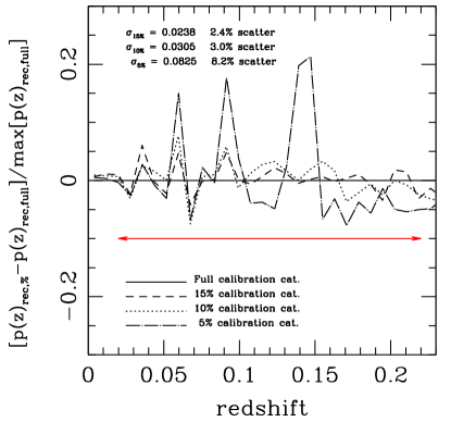
Figure 10: Convergence study of the reconstructed solutions presented in Figure 9, for different spectroscopic “degradation” levels. The root mean square fluctuations of the difference expressed in the $y$-axis are also given, in the redshift range $0.02\leq z\leq 0.22$ denoted by the horizontal arrow, as explained in the main text.

4.3 Can we use Gaussian approximations?

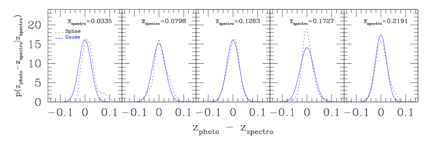
Figure 11: Measurements of the conditional probabilities $p(\zeta-z|z)$’s for five different redshift bins, as indicated in the panels. Dotted lines are spline fits to the pdf’s (the full early-type catalog is used), solid lines are unbiased Gaussian approximations with widths determined by quadratically averaging the SDSS photo-$z$ quoted errors within each redshift bin.

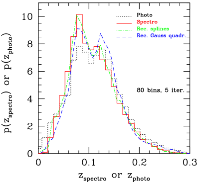
Figure 12: Reconstruction of the redshift distribution when Gaussian approximations are used for the pdf’s (long-dashed line), as opposed to the case when the pdf’s are measured directly from the data (jagged dot-dashed line).

Suppose now that we are missing spectroscopic information in some redshift interval, but that we have photometry available along with photo-$z$ quoted errors in that range. Can we still use our deconvolution technique? In principle, our method is always readily applicable, provided the knowledge of $p(\zeta|z)$. How can we infer it, given the lack of spectral information? In effect, the reconstruction of the intrinsic redshift distribution depends not only on the calibration sample size and on the size of the photometric redshift error $\delta z$, but also on the shape of the distribution $\delta z$. Without relying on other surveys which may cover missing spectral area, we would need to make some assumptions on its shape. The easiest solution is to derive the conditional distributions $p(\zeta|z)$’s by using quoted photo-$z$ errors. Specifically, one may assume the $p(\zeta|z)$’s to be unbiased (i.e. $\bar{\zeta}\equiv\bar{z}$) Gaussians, with widths $\sigma_{\rm z,i}$ determined by quadratically averaging the SDSS photo-$z$ quoted errors within each redshift bin. The question arises as to whether this is a good approximation or not, since there is no a priori reason for the error distributions to be Gaussian and unbiased (Oyaizu et al. 2008). We test this idea on the early-type “calibration” catalog, and the result is displayed in Figure 11. In each panel, we show with dotted lines spline fits to the error probability functions measured from the early-type catalog (all the spectral information is used in this case), and with solid lines their unbiased Gaussian approximations. As it appears evident from the figure, Gaussian approximations are almost always reasonable fits to the data (excluding small tail departures or catastrophic photo-$z$ failures), but with the exception of the redshift interval $z_{\rm spectro}=0.1727$, where the Gaussian fit is rather poor. Unfortunately, this departure is sufficient to make the overall reconstruction of the intrinsic redshift distribution problematic. In Figure 12 we show, with long-dashed lines, the outcome of the deconvolution algorithm when unbiased Gaussian fits are assumed for the pdf’s, and report again for comparison the accurate reconstruction (jagged dot-dashed line), as described in Section 3.2. The deconvolution is critical particularly in the redshift interval where the Gaussian approximation fails (i.e. around $z_{\rm spectro}=0.1727$), and the overall result is of a poor recovery of the intrinsic relation. Therefore, an accurate knowledge of the distribution of photo-$z$ errors is essential for our method to work.

Nevertheless, improving photo-$z$ uncertainties may help to characterize $p(\zeta|z)$ more accurately. It is also worth noticing that, in complete absence of spectroscopic counterpart, we are in principle still able to apply our technique, provided that we have a physically motivated model for the conditional error distribution. This is the real power of this method. On the opposite, the weighting technique proposed by Lima et al. (2008), which addresses similar goals, always requires the spectroscopic sub-sample to span the entire range of photometric observables covered by the photometric sample.

5 Discussion

Using a selected sample of early-type galaxies from the SDSS DR6, for which both photo-$z$s and spectro-$z$s are known, we applied our one- and two-dimensional deconvolution techniques (Sheth 2007; Rossi & Sheth 2008) to reconstruct the unbiased redshift, magnitude and size distributions, as well as the magnitude-size relation (Section 3).

This is a novel approach in recognizing that theoretical predictions, such as the difference between photometric and spectroscopic distance estimates, can be represented as integral equations and solved using deconvolution techniques. In the past, these techniques have been used only observationally, for instance in handling the PSF of telescopes.

We showed that our technique recovers all the true distributions and the joint relation, to a good degree of accuracy. We discussed the magnitude dependence of the error conditional probabilities (Section 3.2), and argued that the problem of reconstructing the true magnitude or size distribution is best thought of as a one-dimensional deconvolution problem (Sections 3.3 and 3.4). We showed that even if the distribution of physical sizes is not severely biased, a significant bias in the magnitude distribution suffices to compromise the size-luminosity relation (Section 3.5). We used our 2D deconvolution technique to correct for this effect.

We then discuss how to extend our procedure to deep redshift catalogs, where limited spectroscopic information, or only photometric data, is available (Section 4). For this part, we performed two tests using the early-type “calibration” sample. We found that using only $10\%$ of the spectroscopic information randomly spaced in our catalog is sufficient for the reconstructions to be accurate with about $3\%$ scatter, when the error in the photometric redshift is typically $\delta z\simeq 0.038$. We also showed that assuming unbiased Gaussians for the $p(\zeta|z)$’s distributions, with widths determined by quadratically averaging the SDSS photo-$z$ quoted errors within each redshift bin, is not always a good approximation. However we argued that, provided one has a detailed knowledge of the pdf from other surveys or from empirically motivated models (see for instance van der Wel et al. 2009), our technique can still be used, even when the spectroscopic sample does not span the entire range of photometric observables covered by the photometric sample.

We address in more detail the problem of handling photo-$z$s when spectroscopic information is missing (for example using a “blind” deconvolution approach) in a forthcoming publication, where we also apply our technique to reconstruct the luminosity function in deep redshift catalogs such as the MegaZ-LRG (Collister et al. 2007).

Even though our discussion was mainly phrased in terms of fundamental distributions and scaling relations for early-type galaxies, so it may be useful for detailed studies of early-types (for example van den Bosch & van de Ven 2008; Bernardi 2009), the method developed here is quite general and can be applied to recover any intrinsic correlations between distance-dependent quantities (even for $n$-correlated variables); potentially, it can impact a broader range of studies, when at least one distance-dependent quantity is involved. In fact, our algorithms can be readily adapted to study the luminosity function in relatively shallow peculiar velocity surveys with noisy Fundamental Plane or $D_{\rm n}-\sigma$ distance estimates (Faber et al. 2007; Tully et al. 2009), or to handle correctly uncertainties in supernova measurements (Krauss et al. 2007; Frieman et al. 2008; Sako et al. 2008), which can bias the redshift-dependent equation of state (Bridle & King 2007; Fosalba & Dore 2007).

A variety of other correlations can be re-analyzed along these lines (see for example Saracco et al. 2009), such as the $R-L$ relation for blue galaxies (Melbourne et al. 2007), the photometric Fundamental Plane (Bolton et al. 2007), and also correlations that do not involve luminosity, such as the Kormendy (1977) relation.Other possible applications involve quasars (Croom et al. 2009; Richards et al. 2009), black-hole $M-L$ correlations, correlations with environment, and potentially future baryonic acoustic oscillation and dark energy surveys.

Appendix A Direct Reconstructions

A widely used method for extracting the redshift probability distribution function (PDFz) from a $\chi^{2}$ minimization is the following (see for example Bolzonella et al. 2000). A $\chi^{2}$ is formed, typically as

$$\chi^{2}=\sum_{\rm f=1}^{\rm N_{f}}\Big{(}{F_{\rm obs}^{\rm f}-A\cdot F_{\rm pred}^{\rm f}(z,T)\cdot 10^{-0.4s_{\rm f}}\over\sigma_{\rm obs}^{\rm f}}\Big{)}^{2}$$ (9)

where $F_{\rm pred}^{f}(z,T)$ is the flux predicted for a template T at redshift z, $F_{\rm obs}^{\rm f}$ is the observed flux, $\sigma_{\rm obs}^{\rm f}$ is the associated error, $f$ refers to each specific filter and $s_{\rm f}$ is the zero-point offset. The photo-$z$ is estimated from the $\chi^{2}$ minimization with respect to the free parameters z, T, and the normalization factor A; namely, the photo-$z$ is the redshift value which minimizes the merit function $\chi^{2}(z,T,A)$. The associated PDFz, or $p(z|\zeta$), is derived from (9),

$$p(z|\zeta)\propto e^{-[\chi^{2}(z)-\chi^{2}_{\rm min}(\zeta)]/2}\,.$$ (10)

There is a main conceptual point in adopting this approach. Photo-$z$s are noisy distance estimates, as opposed to spectroscopic redshifts, which are intrinsic or “true” solutions. Therefore, while $\langle z_{\rm photo}|z_{\rm spectro}\rangle\rightarrow z_{\rm spectro}$ (i.e. convergence of the noisy distribution to the true value), it is certainly not true that $\langle z_{\rm spectro}|z_{\rm photo}\rangle\rightarrow z_{\rm photo}$. This is equivalent to say that the distribution $p(z|\zeta)$, obtained by binning horizontally the plane [$z_{\rm photo}$, $z_{\rm spectro}$] shown in the left panel of Figure 3, is biased by definition. Hence, it is more meaningful to estimate $p(\zeta|z)$ rather than attempting to derive $p(z|\zeta)$.

However, since current photo-$z$ codes output $p(z|\zeta)$ rather than $p(\zeta|z)$, one may wonder if we can apply our technique using the PDFz. In effect, our deconvolution method relies on Bayes’s theorem. For example, if we consider the redshift distribution, application of this theorem yields

$$p(z,\zeta)=N(z)\cdot p(\zeta|z)\equiv p(\zeta,z)={\cal N}(\zeta)\cdot p(z|\zeta).$$ (11)

From the previous relation, it is immediate to show that

$$N(z)=\int{\cal N}(\zeta)~{}p(z|\zeta)~{}{\rm d}\zeta\,.$$ (12)

In this respect, the true (spectroscopic) redshift distribution can be alternatively viewed as a convolution of the noisy photo-$z$ distribution times the PDFz. Therefore, assuming that the PDFz is known from the output of photometric redshift codes and given the observed photo-$z$ distribution, one can obtain the intrinsic $N(z)$ by simply performing the integration (12). This idea is further explored in Sheth & Rossi (2009), where examples of these calculations are presented using the SDSS sample described here.

Similarly, one can obtain the magnitude distribution with a direct integration, since

$$N(M)=\int{\cal N}({\cal M})~{}p(M|{\cal M})~{}{\rm d}{\cal M}\,,$$ (13)

and in principle recover scaling relations as well. However, we would like to remind the reader that when dealing with a real dataset, a noisy observation needs to be “deconvolved” into an intrinsic signal, namely from ${\cal N}(\zeta)$ one needs to reconstruct $N(z)$; $p(z|\zeta)$ is usually not known while $p(\zeta|z)$ can be inferred reliably with a proper “spectroscopic training set” – this is our main motivation for providing a deconvolution approach.

References

- (1)
- Banerji et al. (2008) Banerji, M., Abdalla, F. B., Lahav, O., & Lin, H. 2008, MNRAS, 386, 1219
- Bernardi et al. (2003) Bernardi M., et al., 2003, AJ, 125, 1849
- Bernardi (2009) Bernardi, M. 2009, MNRAS, 510
- Bernstein & Huterer (2009) Bernstein, G., & Huterer, D. 2009, arXiv:0902.2782
- Blanton et al. (2001) Blanton, M. R., et al. 2001, AJ, 121, 235
- Blanton et al. (2003) Blanton, M. R., et al. 2003, ApJ, 592, 819
- Bridle & King (2007) Bridle, S., & King, L. 2007, New Journal of Physics, 9, 444
- Bolton et al. (2007) Bolton, A. S., Burles, S., Treu, T., Koopmans, L. V. E., & Moustakas, L. A. 2007, ApJ, 665, L105
- Bolzonella et al. (2000) Bolzonella, M., Miralles, J.-M., & Pelló, R. 2000, AA, 363, 476
- Budavári et al. (2000) Budavári, T., Szalay, A. S., Connolly, A. J., Csabai, I., & Dickinson, M. 2000, AJ, 120, 1588
- Budavári (2009) Budavári, T. 2009, ApJ, 695, 747
- Carliles et al. (2008) Carliles, S., Budavári, T., Heinis, S., Priebe, C., & Szalay, A. 2008, Astronomical Data Analysis Software and Systems XVII, 394, 521
- Coleman et al. (1980) Coleman, G. D., Wu, C.-C., & Weedman, D. W. 1980, ApJS, 43, 393
- Collister et al. (2007) Collister, A., et al. 2007, MNRAS, 375, 68
- Connolly & Szalay (1999) Connolly, A. J., & Szalay, A. S. 1999, AJ, 117, 2052
- Croom et al. (2009) Croom, S. M., et al. 2009, MNRAS, 392, 19
- Csabai et al. (2003) Csabai, I., et al. 2003, AJ, 125, 580
- Faber et al. (2007) Faber, S. M., et al. 2007, ApJ, 665, 265
- Feldmann et al. (2006) Feldmann, R., et al. 2006, MNRAS, 372, 565
- Fosalba & Doré (2007) Fosalba, P., & Doré, O. 2007, Phys. Rev. D, 76, 103523
- Frieman et al. (2008) Frieman, J. A., et al. 2008, AJ, 135, 338
- Hildebrandt et al. (2008) Hildebrandt, H., Wolf, C., & Benítez, N. 2008, AA, 480, 703
- Hoaglin et al. (1983) Hoaglin, D. C., Mosteller, F., & Tukey, J. W. 1983, Wiley Series in Probability and Mathematical Statistics, New York: Wiley, 1983, edited by Hoaglin, David C.; Mosteller, Frederick; Tukey, John W.,
- Hyde & Bernardi (2009) Hyde, J. B., & Bernardi, M. 2009, MNRAS, 349
- Ilbert et al. (2009) Ilbert, O., et al. 2009, ApJ, 690, 1236
- Jouvel et al. (2009) Jouvel, S., et al. 2009, arXiv:0902.0625
- Krauss et al. (2007) Krauss, L. M., Jones-Smith, K., & Huterer, D. 2007, New Journal of Physics, 9, 141
- Kormendy (1977) Kormendy, J. 1977, ApJ, 218, 333
- Lilly et al. (2007) Lilly, S. J., et al. 2007, ApJS, 172, 70
- Lima et al. (2008) Lima, M., Cunha, C. E., Oyaizu, H., Frieman, J., Lin, H., & Sheldon, E. S. 2008, MNRAS,390, 118
- Lucy (1974) Lucy L. B., 1974, AJ, 79, 745
- Ma & Bernstein (2008) Ma, Z., & Bernstein, G. 2008, ApJ, 682, 39
- Mandelbaum et al. (2008) Mandelbaum, R., et al. 2008, MNRAS, 386, 781
- Melbourne et al. (2007) Melbourne, J., Phillips, A. C., Harker, J., Novak, G., Koo, D. C., & Faber, S. M. 2007, ApJ, 660, 81
- Oyaizu et al. (2008) Oyaizu, H., Lima, M., Cunha, C. E., Lin, H., Frieman, J., & Sheldon, E. S. 2008, ApJ, 674, 768
- Oyaizu et al. (2008) Oyaizu, H., Lima, M., Cunha, C. E., Lin, H., & Frieman, J. 2008, ApJ, 689, 709
- Padmanabhan et al. (2005) Padmanabhan, N., et al. 2005, MNRAS, 359, 237
- Park & Choi (2005) Park, C., & Choi, Y.-Y. 2005, ApJ, 635, L29
- Richards et al. (2009) Richards, G. T., et al. 2009, ApJS, 180, 67
- Rossi & Sheth (2008) Rossi, G., & Sheth, R. K. 2008, MNRAS, 387, 735
- Salvato et al. (2009) Salvato, M., et al. 2009, ApJ, 690, 1250
- Sako et al. (2008) Sako, M., et al. 2008, AJ, 135, 348
- Saracco et al. (2009) Saracco, P., Longhetti, M., & Andreon, S. 2009, MNRAS, 392, 718
- Schmidt (1968) Schmidt, M. 1968, ApJ, 151, 393
- Sheth (2007) Sheth, R. K. 2007, MNRAS, 378, 709
- Sheth & Rossi (2009) Sheth, R. K., & Rossi, G. 2009, MNRAS, submitted
- Stabenau et al. (2008) Stabenau, H. F., Connolly, A., & Jain, B. 2008, MNRAS, 387, 1215
- Sun et al. (2009) Sun, L., Fan, Z.-H., Tao, C., Kneib, J.-P., Jouvel, S., & Tilquin, A. 2009, ApJ, 699, 958
- Tully et al. (2009) Tully, R. B., Rizzi, L., Shaya, E. J., Courtois, H. M., Makarov, D. I., & Jacobs, B. A. 2009, AJ, 138, 323
- van den Bosch & van de Ven (2008) van den Bosch, R. C. E., & van de Ven, G. 2008, arXiv:0811.3474
- van der Wel et al. (2009) van der Wel, A., Bell, E. F., van den Bosch, F. C., Gallazzi, A., & Rix, H.-W. 2009, ApJ, 698, 1232
- Yasuda et al. (2001) Yasuda, N., et al. 2001, AJ, 122, 1104