On convergence rates equivalency and sampling strategies in functional deconvolution models

Abstract

Using the asymptotical minimax framework, we examine convergence rates equivalency between a continuous functional deconvolution model and its real-life discrete counterpart over a wide range of Besov balls and for the $L^{2}$-risk. For this purpose, all possible models are divided into three groups. For the models in the first group, which we call uniform, the convergence rates in the discrete and the continuous models coincide no matter what the sampling scheme is chosen, and hence the replacement of the discrete model by its continuous counterpart is legitimate. For the models in the second group, to which we refer as regular, one can point out the best sampling strategy in the discrete model, but not every sampling scheme leads to the same convergence rates; there are at least two sampling schemes which deliver different convergence rates in the discrete model (i.e., at least one of the discrete models leads to convergence rates that are different from the convergence rates in the continuous model). The third group consists of models for which, in general, it is impossible to devise the best sampling strategy; we call these models irregular.

We formulate the conditions when each of these situations takes place. In the regular case, we not only point out the number and the selection of sampling points which deliver the fastest convergence rates in the discrete model but also investigate when, in the case of an arbitrary sampling scheme, the convergence rates in the continuous model coincide or do not coincide with the convergence rates in the discrete model. We also study what happens if one chooses a uniform, or a more general pseudo-uniform, sampling scheme which can be viewed as an intuitive replacement of the continuous model. Finally, as a representative of the irregular case, we study functional deconvolution with a boxcar-like blurring function since this model has a number of important applications. All theoretical results presented in the paper are illustrated by numerous examples; many of which are motivated directly by a multitude of inverse problems in mathematical physics where one needs to recover initial or boundary conditions on the basis of observations from a noisy solution of a partial differential equation. The theoretical performance of the suggested estimator in the multichannel deconvolution model with a boxcar-like blurring function is also supplemented by a limited simulation study and compared to an estimator available in the current literature. The paper concludes that in both regular and irregular cases one should be extremely careful when replacing a discrete functional deconvolution model by its continuous counterpart.

and

t1Supported in part by NSF Grants DMS-05-05133 and DMS-06-52524.

1 Introduction

We consider the estimation problem of the unknown response function $f(\cdot)$ based on observations from the following noisy convolutions:

$$y(u,t)=f*g(u,t)+\frac{1}{\sqrt{n}}z(u,t),\qquad u\in U,t\in T,$$ (1)

where $U=[a,b]$, $-\infty<a\leq b<\infty$ and $T=[0,1]$. Here, $z(u,t)$ is assumed to be a two-dimensional Gaussian white noise, that is, a generalized two-dimensional Gaussian field with covariance function ${\mathbb{E}}[z(u_{1},t_{1})z(u_{2},t_{2})]=\delta(u_{1}-u_{2})\delta(t_{1}-t_{2})$, where $\delta(\cdot)$ denotes the Dirac $\delta$-function, and

$$f*g(u,t)=\int_{T}f(x)g(u,t-x)\,dx$$

with the blurring (or kernel) function $g(\cdot,\cdot)$ also assumed to be known.

The model (1) has been recently introduced by Pensky and Sapatinas (2009a) and can be viewed as a functional deconvolution model. If $a=b$, it reduces to the standard deconvolution model which attracted the attention of a number of researchers, for example, Donoho (1995), Abramovich and Silverman (1998), Kalifa and Mallat (2003), Johnstone et al. (2004), Donoho and Raimondo (2004), Johnstone and Raimondo (2004), Neelamani, Choi and Baraniuk (2004), Kerkyacharian, Picard and Raimondo (2007), Cavalier and Raimondo (2007) and Chesneau (2008).

The functional deconvolution model (1) can be viewed as a generalization of a multitude of inverse problems in mathematical physics where one needs to recover initial or boundary conditions on the basis of observations of a noisy solution of a partial differential equation. Lattes and Lions (1967) initiated research in the problem of recovering the initial condition for parabolic equations based on observations in a fixed-time strip, while this problem and the problem of recovering the boundary condition for elliptic equations based on observations in an internal domain were studied in Golubev and Khasminskii (1999); the latter problem was also discussed in Golubev (2004). These and other specific models in mathematical physics were discussed in detail in Pensky and Sapatinas (2009a).

However, model (1) is just an idealization of a real-life situation. One can make observations only at particular points $(u_{l},t_{i})$, $l=1,2,\ldots,M$, $i=1,2,\ldots,N$, so that the actual problem can be formulated as follows: recover the unknown response function $f(\cdot)$ from observations $y(u_{l},t_{i})$, where

$$y(u_{l},t_{i})=\int_{T}f(x)g(u_{l},t_{i}-x)\,dx+\varepsilon_{li},\qquad u_{l}\in U,t_{i}=i/N,$$ (2)

with $\varepsilon_{li}$ being standard Gaussian random variables, independent for different $l$ and $i$. Model (2) can be viewed as a discrete version of the continuous functional deconvolution model (1).

It is well documented in the literature that asymptotic equivalence between discrete and continuous models holds in some nonparametric models. In particular, Brown and Low (1996) and Brown et al. (2002) in the univariate case and Reiss (2008) in the multivariate case established, under some restrictions, asymptotic equivalence (in the Le Cam sense) between nonparametric regression and Gaussian white noise models. Although, to the best of our knowledge, such an asymptotic equivalence between continuous and discrete models, in the functional deconvolution setting, has not yet been explored, it has been documented in the literature a convergence rate equivalency, in the asymptotical minimax sense, between standard continuous and discrete deconvolution models, that is, when $a=b$, $M=1$ and $N=n$ in (1) and (2), over a wide range of Besov balls and for the $L^{r}$-risks, $1\leq r<\infty$ [e.g., Chesneau (2008), Pensky and Sapatinas (2009a) and Petsa and Sapatinas (2009)].

For the above reason, and using the asymptotical minimax framework, one may attempt to study the continuous functional deconvolution model (1) instead of its discrete counterpart (2), assuming that the convergence rates between these models coincide. However, in this case, this equivalence has only a limited scope. Indeed, Pensky and Sapatinas (2009a) only touched upon the issue, showing that, under very restrictive conditions, a convergence rate equivalence between the continuous functional deconvolution model (1) and its discrete counterpart (2) models holds when $n=NM$, over a wide range of Besov balls and for the $L^{2}$-risk. Nevertheless, in majority of practical situations, these conditions are violated and it remains to be seen how legitimate the replacement of the real life model (2) by its idealization (1) is, even in the case of inverse problems in mathematical physics, presented in Pensky and Sapatinas (2009a). In fact, in many situations, the convergence rates in the two models depend on the choice of $M$ and the selection of sampling points $u_{1},u_{2},\ldots,u_{M}$ and may coincide with the convergence rates in the continuous model for one selection and be different for another. Also, from a practical point of view, the objective is not to find $M$ and $u_{1},u_{2},\ldots,u_{M}$ which make the two models equivalent from the convergence rate viewpoint, but rather to point out $M$ and $u_{1},u_{2},\ldots,u_{M}$ which deliver the fastest possible convergence rates in the real life model (2). Note that the discrete model (2) can also be viewed as a multichannel deconvolution model where the number of channels $M=M_{n}$ is fixed or, possibly, $M_{n}\rightarrow\infty$ as the sample size $n\rightarrow\infty$; the case when $M\geq 2$ (finite) was considered in, for example, Casey and Walnut (1994) and De Canditiis and Pensky (2004, 2006). Hence if the kernel $g(\cdot,\cdot)$ is fixed, the choice of $M$ and the selection of sampling points $u_{1},u_{2},\ldots,u_{M}$ which provide the fastest convergence rates is of extreme importance in signal processing.

Using the asymptotical minimax framework, our objective is to evaluate how legitimate it is to replace the real-life discrete model (2) by its continuous counterpart (1). For this purpose, we shall divide all possible models into three groups. For the models in the first group, which we call uniform, the convergence rates in discrete and continuous functional deconvolution models coincide no matter what the sampling scheme is chosen, and hence the replacement of the discrete model by its continuous counterpart is legitimate. For the models in the second group, to which we refer as regular, one can point out the best sampling strategy in the discrete model (i.e., the strategy which leads to the fastest convergence rate), but not every sampling scheme leads to the same convergence rates: there are at least two sampling schemes which deliver different convergence rates in the discrete model (i.e., at least one of the discrete models leads to convergence rates that are different from the convergence rates in the continuous functional deconvolution model). The third group consists of models for which, in general, it is impossible to devise the best sampling strategy; we call these models irregular.

We formulate the conditions when each of these situations takes place. In the regular case, we not only point out the choice of $M$ and the selection of sampling points $u_{1},u_{2},\ldots,u_{M}$ which deliver the fastest convergence rates in the discrete model but also investigate when, in the case of an arbitrary sampling scheme, the convergence rates in the continuous functional deconvolution model coincide or do not coincide with the convergence rates of its discrete counterpart. We also study what happens if one chooses a uniform, or a more general pseudo-uniform, sampling scheme which can be viewed as an intuitive replacement of the continuous model. Finally, as a representative of the irregular case, we study functional deconvolution with a boxcar-like kernel since this model has a number of important applications. All theoretical results presented are illustrated by numerous examples; many of which are motivated directly by a multitude of inverse problems in mathematical physics where one needs to recover initial or boundary conditions on the basis of observations from a noisy solution of a partial differential equation.

As in Pensky and Sapatinas (2009a), we consider functional deconvolution in a periodic setting; that is, we assume that $f(\cdot)$ and, for fixed $u\in U$, $g(u,\cdot)$ are periodic functions with period on the unit interval $T$. Note that the periodicity assumption appears naturally in the above mentioned special models which (1) and (2) generalize and allows one to explore ideas considered in the above cited papers to the proposed functional deconvolution framework. Moreover, not only for theoretical reasons but also for practical convenience [see Johnstone et al. (2004), Sections 2.3, 3.1 and 3.2], we use band-limited wavelet bases and in particular the periodized Meyer wavelet basis for which fast algorithms exist [see Kolaczyk (1994) and Donoho and Raimondo (2004)]. In order to also allow inhomogeneous functions $f(\cdot)$ into our study, we consider a wide range of Besov balls, as it is common in the wavelet literature, and, for simplicity, we work with the $L^{2}$-risk only. However, the results of this paper can be extended to a more general class of $L^{r}$-risks, $1\leq r<\infty$, using the unconditionality and Temlyakov properties of Meyer wavelets [e.g., Johnstone et al. (2004) and Petsa and Sapatinas (2009)].

The rest of the paper is organized as follows. In Section 2, we describe the construction of wavelet estimators of $f(\cdot)$ derived by Pensky and Sapatinas (2009a) both for the continuous functional deconvolution model (1) and its discrete counterpart (2). In Section 3, for the continuous model and for a discrete model with any particular design of sampling points, using the asymptotical minimax framework, we provide lower bounds for the $L^{2}$-risk over a wide range of Besov balls and show that those bounds are attained by the wavelet estimators constructed in Section 2. Section 4 is devoted to the discussion of the interplay between continuous and discrete functional deconvolution models. First, Section 4.1 formulates the necessary and sufficient conditions for the convergence rates in continuous and discrete functional deconvolution models to coincide and to be independent of the choice of $M$ and the selection of points $u_{1},u_{2},\ldots,u_{M}$. Then Section 4.2 provides examples where these conditions do or do not take place, and Section 4.3 sorts all possible situations into the uniform, regular and irregular cases. Section 5 studies the regular case. In particular, Section 5.1 designs the best possible sampling strategy. Section 5.2 provides some motivating examples. Section 5.3 investigates the relation between the $L^{2}$-risks in the continuous and the discrete models under an arbitrary sampling scheme and formulates conditions when the convergence rates do or do not coincide. Section 5.4 formulates sufficient conditions when the convergence rates in both models coincide under a pseudo-uniform sampling scheme in the discrete model. Section 5.5 provides a variety of examples where the convergence rates coincide or differ depending on what sampling scheme is employed. Section 6 explores the interplay between continuous and discrete functional deconvolution models in the case of a boxcar-like blurring function. Section 7 supplements the theory with a limited simulation study in the case of a boxcar-like blurring function and compares performance of the suggested estimator to the estimator proposed by De Canditiis and Pensky (2006). Concluding remarks are given in Section 8. Finally, the Appendix provides the proofs of the theoretical results obtained in the previous sections.

In the rest of the paper, the continuous functional deconvolution model (1) is referred to as the “continuous model” and its discrete counterpart (2) is referred to as the “discrete model.”

2 Wavelet estimators

For both the continuous model and the discrete model, we use the wavelet estimator derived in Pensky and Sapatinas (2009a), described as follows.

Let $\varphi^{*}(\cdot)$ and $\psi^{*}(\cdot)$ be the Meyer scaling and mother wavelet functions, respectively, in the real line [see, e.g., Meyer (1992)] and obtain a periodized version of Meyer wavelet basis as in Johnstone et al. (2004); that is, for $j\geq 0$ and $k=0,1,\ldots,2^{j}-1$,

$$\varphi_{jk}(x) = \sum_{i\in\mathbb{Z}}2^{j/2}\varphi^{*}\bigl{(}2^{j}(x+i)-k\bigr{)},$$

$$\psi_{jk}(x) = \sum_{i\in\mathbb{Z}}2^{j/2}\psi^{*}\bigl{(}2^{j}(x+i)-k\bigr{)},\qquad x\in T.$$

Denote $\langle f,g\rangle=\int_{T}f(t)\overline{g(t)}\,dt$, the inner product in the Hilbert space $L^{2}(T)$. Let $e_{m}(t)=e^{i2\pi mt}$, $m\in\mathbb{Z}$, and, for any (primary resolution level) $j_{0}\geq 0$ and any $j\geq j_{0}$, let $\varphi_{mj_{0}k}=\langle e_{m},\varphi_{j_{0}k}\rangle,\psi_{mjk}=\langle e_{m},\psi_{jk}\rangle,f_{m}=\langle e_{m},f\rangle$ be the Fourier coefficients of $\varphi_{jk}(\cdot)$, $\psi_{jk}(\cdot)$ and $f(\cdot)$, respectively. For each $u\in U$, denote the functional Fourier coefficients by

$$y_{m}(u)=\langle e_{m},y(u,\cdot)\rangle,\qquad g_{m}(u)=\langle e_{m},g(u,\cdot)\rangle.$$

In what follows we assume that function $g(u,t)$ is such that $g_{m}(u)$ are continuous functions of $u$ for every $m$. (This condition is not restrictive and holds in all examples considered below.)

If we have the continuous model (1), then, by using properties of the Fourier transform, for each $u\in U$, we have $h_{m}(u)=g_{m}(u)f_{m}$ and

$$y_{m}(u)=g_{m}(u)f_{m}+n^{-1/2}z_{m}(u),$$ (3)

where $z_{m}(u)$ are generalized one-dimensional (complex-valued) Gaussian processes such that ${\mathbb{E}}[z_{m_{1}}(u_{1})\overline{z_{m_{2}}(u_{2})}]=\delta_{m_{1},m_{2}}\delta(u_{1}-u_{2})$, where $\delta_{m_{1},m_{2}}$ is Kronecker’s delta. If we have the discrete model (2), then, by using properties of the discrete Fourier transform, for each $l=1,2,\ldots,M$, (3) takes the form

$$y_{m}(u_{l})=g_{m}(u_{l})f_{m}+N^{-1/2}z_{ml},$$ (4)

where $z_{ml}$ are standard (complex-valued) Gaussian random variables, independent for different $m$ and $l$.

Estimate the Fourier coefficients $f_{m}$ of $f(\cdot)$ by

$$\hat{f}_{m} = \biggl{(}\int_{a}^{b}\overline{g_{m}(u)}y_{m}(u)\,du\biggr{)}\bigg{/}\biggl{(}\int_{a}^{b}|g_{m}(u)|^{2}\,du\biggr{)}$$

$$\eqntext{\mbox{in the continuous model},}$$ (6)

$$\hat{f}_{m} = \Biggl{(}\sum_{l=1}^{M}\overline{g_{m}(u_{l})}y_{m}(u_{l})\Biggr{)}\Bigg{/}\Biggl{(}\sum_{l=1}^{M}|g_{m}(u_{l})|^{2}\Biggr{)}$$

$$\eqntext{\mbox{in the discrete model.}}$$ (8)

Here, we adopt the convention that when $a=b$, $\hat{f}_{m}$ takes the form $\hat{f}_{m}=(\overline{g_{m}(a)}y_{m}(a)/|g_{m}(a)|^{2}$ and somewhat abuse notation using $f_{m}$ for both functional Fourier coefficients and their discrete counterparts.

Note that, using the periodized Meyer wavelet basis described above and for any $j_{0}\geq 0$, any (periodic) $f(\cdot)\in L^{2}(T)$ can be expanded as

$$f(t)=\sum_{k=0}^{2^{j_{0}}-1}a_{j_{0}k}\varphi_{j_{0}k}(t)+\sum_{j=j_{0}}^{\infty}\sum_{k=0}^{2^{j}-1}b_{jk}\psi_{jk}(t),\qquad t\in T.$$ (9)

Furthermore, by Plancherel’s formula, the scaling coefficients, $a_{j_{0}k}=\langle f,\varphi_{j_{0}k}\rangle$, and the wavelet coefficients, $b_{jk}=\langle f,\psi_{jk}\rangle$, of $f(\cdot)$ can be represented as

$$a_{j_{0}k}=\sum_{m\in C_{j_{0}}}f_{m}\overline{\varphi_{mj_{0}k}},\qquad b_{jk}=\sum_{m\in C_{j}}f_{m}\overline{\psi_{mjk}},$$ (10)

where $C_{j_{0}}=\{m\dvtx\varphi_{mj_{0}k}\neq 0\}$ and, for any $j\geq j_{0}$, $C_{j}=\{m\dvtx\psi_{mjk}\neq 0\}$. We estimate $a_{j_{0}k}$ and $b_{jk}$ by substituting $f_{m}$ in (10) with (2) or (2), that is,

$$\hat{a}_{j_{0}k}=\sum_{m\in C_{j_{0}}}\hat{f}_{m}\overline{\varphi_{mj_{0}k}},\qquad\hat{b}_{jk}=\sum_{m\in C_{j}}\hat{f}_{m}\overline{\psi_{mjk}}.$$ (11)

We now construct a (block thresholding) wavelet estimator of $f(\cdot)$, suggested by Pensky and Sapatinas (2009a). For this purpose, we divide the wavelet coefficients at each resolution level into blocks of length $\ln n$. Let $A_{j}$ and $U_{jr}$ be the following sets of indices: $A_{j}=\{r\mid r=1,2,\ldots,2^{j}/\ln n\},$ $U_{jr}=\{k\mid k=0,1,\ldots,2^{j}-1;(r-1)\ln n\leq k\leq r\ln n-1\}.$ Denote

$$B_{jr}=\sum_{k\in U_{jr}}b_{jk}^{2},\qquad\hat{B}_{jr}=\sum_{k\in U_{jr}}\hat{b}_{jk}^{2}.$$ (12)

Finally, for any $j_{0}\geq 0$, $f(\cdot)$ is constructed as

$$\hat{f}_{n}(t) = \sum_{k=0}^{2^{j_{0}}-1}\hat{a}_{j_{0}k}\varphi_{j_{0}k}(t)$$

$${}+\sum_{j=j_{0}}^{J-1}\sum_{r\in A_{j}}\sum_{k\in U_{jr}}\hat{b}_{jk}{\mathbb{I}}(|\hat{B}_{jr}|\geq\lambda_{j})\psi_{jk}(t),\qquad t\in T,$$

where ${\mathbb{I}}(A)$ is the indicator function of the set $A$, and the resolution levels $j_{0}$ and $J$ and the thresholds $\lambda_{j}$ will be defined in Section 3.2.

In what follows, the symbol $C$ is used for a generic positive constant, independent of $n$, while the symbol $K$ is used for a generic positive constant, independent of $m$, $n$, $M$ and $u_{1},u_{2},\ldots,u_{M}$, which either of them may take different values at different places.

3 Minimax lower and upper bounds for the $L^{2}$-risk over Besov balls

Among the various characterizations of Besov spaces for periodic functions defined on $L^{p}(T)$ in terms of wavelet bases, we recall that for an $r$-regular multiresolution analysis with $0<s<r$ and for a Besov ball, $B_{p,q}^{s}(A)=\{f(\cdot)\in L^{p}(T)\dvtx f\in B_{p,q}^{s},\|f\|_{B_{p,q}^{s}}\leq A\}$, of radius $A>0$ with $1\leq p,q\leq\infty$, one has that, with $s^{\prime}=s+1/2-1/p$,

$$B_{p,q}^{s}(A) = \Biggl{\{}f(\cdot)\in L^{p}(T)\dvtx\Biggl{(}{\sum_{k=0}^{2^{j_{0}}-1}}|a_{j_{0}k}|^{p}\Biggr{)}^{{1}/{p}}$$

$$\hskip 4.8pt{}+\Biggl{(}\sum_{j=j_{0}}^{\infty}2^{js^{\prime}q}\Biggl{(}{\sum_{k=0}^{2^{j}-1}|b_{jk}}|^{p}\Biggr{)}^{q/p}\Biggr{)}^{{1/q}}\leq A\Biggr{\}}$$

with respective sum(s) replaced by maximum if $p=\infty$ or $q=\infty$ [see, e.g., Johnstone et al. (2004), Section 2.4]. (Note that, for the Meyer wavelet basis, considered in Section 2, $r=\infty$.)

We construct below asymptotical minimax lower bounds for the $L^{2}$-risk based on observations from either the continuous model or the discrete model. For this purpose, we define the corresponding minimax $L^{2}$-risks over the set $\Omega$ as

$$R_{n}^{c}(\Omega) = \inf_{\tilde{f}_{n}^{c}}\sup_{f\in\Omega}{\mathbb{E}}\|\tilde{f}_{n}^{c}-f\|^{2},$$ (15)

$$R_{n}^{d}(\Omega,\underline{u},M) = \inf_{\tilde{f}_{n}^{d}}\sup_{f\in\Omega}{\mathbb{E}}\|\tilde{f}_{n}^{d}-f\|^{2},$$ (16)

$$R_{n}^{d}(\Omega) = \inf_{\underline{u},M}R_{n}^{d}(\Omega,\underline{u},M),$$ (17)

where the infimum in (15) is taken over all possible estimators (i.e., measurable functions) $\tilde{f}_{n}^{c}(\cdot)$ of $f(\cdot)$ from the continuous model, the infimum in (17) is taken over all possible estimators $\tilde{f}_{n}^{d}(\cdot)$ of $f(\cdot)$ from the discrete model, based on a sample at $M$ points $\underline{u}=(u_{1},u_{2},\ldots,u_{M})$ and the infimum in (17) is evaluated over all possible estimators $\tilde{f}_{n}^{d}(\cdot)$ of $f(\cdot)$ and the choices of $M$ and $\underline{u}$. Note that, since the asymptotical minimax convergence rates for the $L^{2}$-risk in the discrete model depends on $M$ and $\underline{u}$ if these quantities are fixed, we are interested in the selection of $M$ and $\underline{u}$, minimizing the asymptotical minimax convergence rates for the $L^{2}$-risk.

Denote $s^{*}=s+1/2-1/p^{\prime},p^{\prime}=\min(p,2)$ and, for $\kappa=1,2$, define

$$\quad\tau_{\kappa}^{c}(m)={\int_{a}^{b}}|g_{m}(u)|^{2\kappa}\,du\quad\mbox{and}\quad\tau_{\kappa}^{d}(m,\underline{u},M)=\frac{1}{M}\sum_{l=1}^{M}|g_{m}(u_{l})|^{2\kappa},$$ (18)

where $\tau_{1}^{c}(m)=|g_{m}(a)|^{2}$ when $a=b$.

Pensky and Sapatinas (2009a) constructed asymptotical minimax lower and upper bounds for the $L^{2}$-risk for the continuous model. The corresponding bounds for the discrete model were obtained under the very restrictive conditions that the upper and the lower bounds on $\tau_{1}^{d}(m,\underline{u},M)$ do not depend on $n$, $M$ and $\underline{u}$. Below we shall need asymptotic lower and upper bounds for the $L^{2}$-risk in the case of much more general expressions for $\tau_{1}^{c}(m)$ and $\tau_{1}^{d}(m,\underline{u},M)$, than in Pensky and Sapatinas (2009a).

3.1 Minimax lower bounds: Particular choice of sampling points

Let, with some abuse of notation, $\tau_{1}(m)=\tau_{1}^{c}(m)$, $R_{n}^{*}(B_{p,q}^{s}(A))=R_{n}^{c}(B_{p,q}^{s}(A))$, in the continuous model, and $\tau_{1}(m)=\tau_{1}^{d}(m,\underline{u},M)$, $R_{n}^{*}(B_{p,q}^{s}(A))=\break R_{n}^{d}(B_{p,q}^{s}(A),\underline{u},M)$, in the discrete model.

Assume that for some constants $\nu\in\mathbb{R}$, $\lambda\in\mathbb{R}$, $\alpha\geq 0$ and $\beta>0$, independent of $m$ and $n$, and for some sequence $\varepsilon_{n}>0$, independent of $m$,

$$\tau_{1}(m)\leq K\varepsilon_{n}|m|^{-2\nu}({\ln}|m|)^{-\lambda}\exp(-\alpha|m|^{\beta}),\qquad\nu>0\mbox{ if }\alpha=0.$$ (19)

Denote ${n^{*}}=n\varepsilon_{n}$ and assume that the sequence $\varepsilon_{n}$ is such that

$${n^{*}}=n\varepsilon_{n}\rightarrow\infty\qquad\mbox{as }n\rightarrow\infty.$$ (20)

Then the following statement is true.

Theorem 1

Let $\{\phi_{j_{0},k}(\cdot),\psi_{j,k}(\cdot)\}$ be the periodic Meyer wavelet basis discussed in Section 2. Let $s>\max(0,1/p-1/2)$, $1\leq p\leq\infty$, $1\leq q\leq\infty$ and $A>0$. Let assumptions (19) and (20) hold. Then, as $n\rightarrow\infty$,

$$R_{n}^{*}(B_{p,q}^{s}(A))\geq\cases{C({n^{*}})^{-{2s}/({2s+2\nu+1})}(\ln{n^{*}})^{{2s\lambda}/({2s+2\nu+1})},\cr\hskip 92.8pt\mbox{if $\alpha=0,\nu(2-p)<p{s^{*}}$,}\cr C\biggl{(}\dfrac{\ln{n^{*}}}{{n^{*}}}\biggr{)}^{{2{s^{*}}}/({2s^{*}+2\nu})}(\ln{n^{*}})^{{2{s^{*}\lambda}}/({2s^{*}+2\nu})},\cr\hskip 92.8pt\mbox{if $\alpha=0,\nu(2-p)\geq p{s^{*}}$,}\cr C(\ln{n^{*}})^{-{2{s^{*}}}/{\beta}},\qquad\mbox{if $\alpha>0$.}}$$ (21)

3.2 Minimax upper bounds: Particular choice of sampling points

Assume that for the constants $\nu\in\mathbb{R}$, $\lambda\in\mathbb{R}$, $\alpha\geq 0$ and $\beta>0$ and the sequence $\varepsilon_{n}>0$ in (19)

$$\tau_{1}(m)\geq K\varepsilon_{n}|m|^{-2\nu}({\ln}|m|)^{-\lambda}\exp(-\alpha|m|^{\beta}),\qquad\nu>0\mbox{ if }\alpha=0.$$ (22)

Let $\hat{f}_{n}(\cdot)$ be the wavelet estimator defined by (2). Let, as before, ${n^{*}}=n\varepsilon_{n}$ satisfy condition (20), and assume that in the case of $\alpha=0$ in (22) the sequence $\varepsilon_{n}$ is such that

$$-h_{1}\ln n\leq\ln(1/\varepsilon_{n})\leq(1-h_{2})\ln n$$ (23)

for some constants $h_{1}>0$ and $h_{2}\in(0,1)$. Observe that condition (23) implies (20) and that $\ln{n^{*}}\asymp\ln n$ as $n\rightarrow\infty$. Here, and in what follows, $u(n)\asymp v(n)$ means that there exist constants $C_{1}>0$ and $C_{2}>0$, independent of $n$, such that $0<C_{1}v(n)\leq u(n)\leq C_{2}v(n)<\infty$ for $n$ large enough.

Choose ${j_{0}}$ and $J$ such that

$$2^{j_{0}} = \ln({n^{*}}),\qquad 2^{J}=({n^{*}})^{{1}/({2\nu+1})}\qquad\mbox{if }\alpha=0,$$ (24)

$$2^{j_{0}} = \frac{3}{8\pi}\biggl{(}\frac{\ln({n^{*}})}{2\alpha}\biggr{)}^{{1}/{\beta}},\qquad 2^{J}=2^{{j_{0}}}\qquad\mbox{if }\alpha>0.$$ (25)

[Since ${j_{0}}>J-1$ when $\alpha>0$, the estimator (2) only consists of the first (linear) part, and hence $\lambda_{j}$ does not need to be selected in this case.] Set, for some constant $\mu>0$, large enough,

$$\lambda_{j}=\mu^{2}({n^{*}})^{-1}\ln({n^{*}})2^{2\nu j}j^{\lambda}\qquad\mbox{if }\alpha=0.$$ (26)

Note that the choices of ${j_{0}}$, $J$ and $\lambda_{j}$ are independent of the parameters, $s$, $p$, $q$ and $A$ of the Besov ball $B_{p,q}^{s}(A)$; hence the estimator (2) is adaptive with respect to these parameters.

Set $(x)_{+}=\max(0,x)$, and define

$$\varrho=\cases{\dfrac{(2\nu+1)(2-p)_{+}}{p(2s+2\nu+1)},&\quad if $\nu(2-p)<p{s^{*}}$,\cr\dfrac{(q-p)_{+}}{q},&\quad if $\nu(2-p)=p{s^{*}}$,\cr 0,&\quad if $\nu(2-p)>p{s^{*}}$.}$$ (27)

For any $j\geq j_{0}$, let $|C_{j}|$ be the cardinality of the set $C_{j}$; note that, for Meyer wavelets, $|C_{j}|=4\pi 2^{j}$ [see, e.g., Johnstone et al. (2004)]. Let also

$$\Delta_{\kappa}(j)=|C_{j}|^{-1}\sum_{m\in C_{j}}\tau_{\kappa}(m)[\tau_{1}(m)]^{-2\kappa},\qquad\kappa=1,2.$$ (28)

Direct calculations yield that under conditions (22) and (23), for some constants $c_{1}>0$ and $c_{2}>0$, independent of $n$, one has

$$\Delta_{1}(j)\leq\cases{c_{1}(\varepsilon_{n})^{-1}2^{2\nu j}j^{\lambda},&\quad if $\alpha=0$,\cr c_{2}(\varepsilon_{n})^{-1}2^{2\nu j}j^{\lambda}\exp\biggl{\{}\alpha\biggl{(}\dfrac{8\pi}{3}\biggr{)}^{\beta}2^{j\beta}\biggr{\}},&\quad if $\alpha>0$.}$$ (29)

The proof of the minimax upper bounds for the $L^{2}$-risk is based on the following two lemmas.

Lemma 1

Let assumption (22) hold, and let the estimators $\hat{a}_{j_{0}k}$ and $\hat{b}_{jk}$ of the scaling and wavelet coefficients $a_{j_{0}k}$ and $b_{jk}$, respectively, be given by the formula (11) with $\hat{f}_{m}$ defined by (2) in the continuous model and by (2) in the discrete model. Then, for all $j\geq j_{0}$,

$$\quad{\mathbb{E}}|\hat{a}_{j_{0}k}-a_{j_{0}k}|^{2}\leq Cn^{-1}\Delta_{1}({j_{0}}),\qquad{\mathbb{E}}|\hat{b}_{jk}-b_{jk}|^{2}\leq Cn^{-1}\Delta_{1}(j).$$ (30)

If $\alpha=0$ and assumption (23) holds, then, for any $j\geq j_{0}$, one has

$${\mathbb{E}}|\hat{b}_{jk}-b_{jk}|^{4}\leq Cn(\ln n)^{3\lambda}({n^{*}})^{-{3}/({2\nu+1})}.$$ (31)

Lemma 2

Let the estimators $\hat{b}_{jk}$ of the wavelet coefficients $b_{jk}$ be given by the formula (11) with $\hat{f}_{m}$ defined by (2) in the continuous model and by (2) in the discrete model. Let assumptions (22) (if $\alpha=0$) and (23) hold. If

$$\mu\geq 2\sqrt{c_{1}}\bigl{(}\sqrt{6}+1\bigr{)}/\sqrt{h_{2}},$$ (32)

where $c_{1}$ and $h_{2}$ are defined in (29) and (23), respectively, then, for all $j\geq j_{0}$,

$${\mathbb{P}}\biggl{(}{\sum_{k\in U_{jr}}}|\hat{b}_{jk}-b_{jk}|^{2}\geq(4{n^{*}})^{-1}\mu^{2}2^{2\nu j}j^{\lambda}\ln({n^{*}})\biggr{)}\leq n^{-3}.$$ (33)

Then the following statement is true.

Theorem 2

Let $\hat{f}_{n}(\cdot)$ be the wavelet estimator defined by (2), with ${j_{0}}$ and $J$ given by (24) (if $\alpha=0$) or (25) (if $\alpha>0$) and $\mu$ satisfying (32). Let $s>1/p^{\prime}$, $1\leq p\leq\infty$, $1\leq q\leq\infty$ and $A>0$. Then, under the assumptions (22) and (20) if $\alpha>0$, or (22) and (23) if $\alpha=0$, as $n\rightarrow\infty$,

$$\sup_{f\in B_{p,q}^{s}(A)}{\mathbb{E}}\|\hat{f}_{n}-f\|^{2}$$

(34)

$$\qquad\leq\cases{C({n^{*}})^{-{2s}/({2s+2\nu+1})}(\ln n)^{\varrho+{2s\lambda}/({2s+2\nu+1})},\cr\hskip 99.37pt\mbox{if $\alpha=0,\nu(2-p)<p{s^{*}}$},\cr C\biggl{(}\dfrac{\ln n}{{n^{*}}}\biggr{)}^{{2{s^{*}}}/({2s^{*}+2\nu})}(\ln n)^{\varrho+{2{s^{*}\lambda}}/({2s^{*}+2\nu})},\cr\hskip 99.37pt\mbox{if $\alpha=0,\nu(2-p)\geq p{s^{*}}$},\cr C(\ln({n^{*}}))^{-{2{s^{*}}}/{\beta}},\qquad\mbox{if $\alpha>0$.}}$$

Remark 1.

Note that in the continuous model, one can write a lower bound for $\tau_{1}(m)$ in (19) and an upper bound for $\tau_{1}(m)$ in (22) with $\varepsilon_{n}=1$, so that ${n^{*}}=n$ in (21) and (2). However, in the discrete model this may not be possible. Theorems 1 and 2 allow to account for the dependence of $\tau_{1}(m)$ on $n$ in the case of the discrete model as well as for an extra logarithmic factor in the expression of $\tau_{1}(m)$ which often appears in the case of the continuous model.

Remark 2.

Note that Theorems 1 and 2 can be applied even if the values of $\nu,\lambda$, $\alpha$ and $\beta$ in assumptions (19) and (22) are different, that may also depend on $M$ and $\underline{u}$. Then Theorem 1 provides asymptotical minimax lower bounds for the $L^{2}$-risk while Theorem 2 provides the corresponding upper bounds. If, in the continuous model or in the discrete model with some particular choice of $M$ and sampling points $\underline{u}$, the values of $\nu,\lambda$, $\alpha$ and $\beta$ and the functions $\varepsilon_{n}$ in conditions (19) and (22) coincide, then Theorems 1 and 2 imply that the estimator $\hat{f}_{n}(\cdot)$ defined by (2) is asymptotically optimal (in the minimax sense), or near-optimal within a logarithmic factor, over a wide range of Besov balls $B_{p,q}^{s}(A)$. Therefore, in the rest of the paper, when we talk about convergence rates we refer to the asymptotical minimax lower bounds for the $L^{2}$-risk which are attainable, up to at most a logarithmic factor, according to Theorems 1 and 2.

4 The interplay between continuous and discrete models: Uniform, regular and irregular cases

The convergence rates in the discrete model depend on two aspects: the total number of observations $n=NM$ and the behavior of $\tau_{1}^{d}(m,\underline{u},M)$. In the continuous model, the values of $\tau_{1}^{c}(m)$ are fixed; they depend on $m$ only, and hence conditions (19) and (22) can be easily verified. However, this is no longer true in the discrete model; in this case, the values of $\tau_{1}^{d}(m,\underline{u},M)$ may depend on the choice of $M$ and the selection of points $\underline{u}$. If we require the values of $\tau_{1}^{d}(m,\underline{u},M)$ to be independent of the choice of $M$ and the selection of points $\underline{u}$, then the convergence rates in the discrete and the continuous models coincide and are independent of the selection of points $\underline{u}$. Moreover, in this case, the wavelet estimator (2) is asymptotically optimal (in the minimax sense) no matter what the choice of $M$ is. It is quite possible, however, that in the discrete model, conditions (19) and (22) both hold but with different values of $\nu$, $\lambda$, $\alpha$ and $\beta$ for different choices of $M$ and $\underline{u}$. In this case, the asymptotical minimax upper bounds for the $L^{2}$-risk in the discrete model may not coincide with the convergence rates in the continuous model, at least for some sampling schemes.

4.1 Necessary and sufficient conditions for convergence rates equivalency between continuous and discrete models

Assume that there exist points $u_{*},u^{*}\in[a,b]$, independent of $m$, such that, for any $u\in[a,b]$,

$$|g_{m}(u)|\leq K|g_{m}(u^{*})|\quad\mbox{and}\quad|g_{m}(u)|\geq K|g_{m}(u_{*})|.$$ (35)

In this case,

$$(b-a)K^{2}|g_{m}(u_{*})|^{2}\leq\tau_{1}^{c}(m)\leq(b-a)K^{2}|g_{m}(u^{*})|^{2}$$

and $K^{2}|g_{m}(u_{*})|^{2}\leq\tau_{1}^{d}(m,\underline{u},M)\leq K^{2}|g_{m}(u^{*})|^{2}$ for any $M$ and $\underline{u}$. Note that, based on the assumption on the blurring function $g(\cdot,\cdot)$ made in Section 2, points $u_{*}$ and $u^{*}$ satisfying condition (35) always exist; however, they are not necessarily independent of $m$.

Here, and in what follows, $u_{m}\asymp v_{m}$ means that there exist constants $C_{1}>0$ and $C_{2}>0$, independent of $m$, such that $0<C_{1}v_{m}\leq u_{m}\leq C_{2}v_{m}<\infty$ for $|m|$ large enough.

The following statement, which substantially extends Proposition 1 of Pensky and Sapatinas (2009a), presents the necessary and sufficient conditions for the convergence rates in the discrete model to be independent of the choice of $M$ and the selection of points $\underline{u}$ and hence to coincide with the convergence rates in the continuous model.

Theorem 3

Let there exist constants $\nu_{1}\in\mathbb{R}$, $\nu_{2}\in\mathbb{R}$, $\alpha_{1}\geq 0$, $\alpha_{2}\geq 0$, $\beta_{1}>0$ and $\beta_{2}>0$, independent of $m$ and $n$, such that

$$|g_{m}(u^{*})|^{2} \asymp |m|^{-2\nu_{1}}\exp(-\alpha_{1}|m|^{\beta_{1}}),\qquad\nu_{1}>0\mbox{ if }\alpha_{1}=0,$$ (36)

$$|g_{m}(u_{*})|^{2} \asymp |m|^{-2\nu_{2}}\exp(-\alpha_{2}|m|^{\beta_{2}}),\qquad\nu_{2}>0\mbox{ if }\alpha_{2}=0.$$ (37)

Then, the convergence rates obtained in Theorems 1 and 2 in the discrete model are independent of the choice of $M$ and the selection of points $\underline{u}$, and hence coincide with the convergence rates obtained in Theorems 1 and 2 in the continuous model, if and only if

$$\alpha_{1}\alpha_{2}>0\quad\mbox{and}\quad\beta_{1}=\beta_{2}\quad\mbox{or}\quad\alpha_{1}=\alpha_{2}=0\quad\mbox{and}\quad\nu_{1}=\nu_{2}.$$ (38)

Remark 3.

Theorem 3 provides necessary and sufficient conditions for the convergence rates in the continuous and the discrete models to coincide, and to be independent of the choice of $M$ and the selection of points $\underline{u}$. These conditions also guarantee asymptotical optimality (in the minimax sense) of the wavelet estimator (2) and can be viewed as some kind of uniformity conditions. Under assumptions (36)–(38), asymptotically (up to a constant factor) it makes absolutely no difference whether one samples the discrete model $n$ times at one point, say, $u_{1}$ or, say, $\sqrt{n}$ times at $M=\sqrt{n}$ points $u_{l}$, $l=1,2,\ldots,M$. In other words, each sample value $y(u_{l},t_{i})$, $l=1,2,\ldots,M$, $i=1,2,\ldots,N$, asymptotically (up to a constant factor) gives the same amount of information, and, therefore, the convergence rates are not sensitive to the choice of $M$ and the selection of points $\underline{u}$. On the other hand, if the conditions of Theorem 3 are violated, then the convergence rates in the discrete model depend on the choice of $M$ and $\underline{u}$, and some recommendations on their selection should be given. Furthermore, optimality (in the minimax sense) issues become much more complex when $\tau_{1}^{d}(m;\underline{u},M)$ is not uniformly bounded from above or below.

4.2 Some illustrative examples

Theorem 3 provides necessary and sufficient conditions for the continuous and the discrete models to be equivalent, from the viewpoint of convergence rates, no matter what the choice of $M$ and the selection of points $\underline{u}$ are. The difficulty, however, is that many models do not satisfy those conditions. Below, we consider some illustrative examples that have recently been studied in Pensky and Sapatinas (2009a).

Example 1 ((Estimation of the initial condition in the heat conductivity equation)).

Let $h(t,x)$ be a solution of the heat conductivity equation,

$$\frac{\partial h(t,x)}{\partial t}=\frac{\partial^{2}h(t,x)}{\partial x^{2}},\qquad x\in[0,1],t\in[a,b],a>0,b<\infty,$$

with initial condition $h(0,x)=f(x)$ and periodic boundary conditions $h(t,0)=h(t,1)$ and $\partial h(t,x)/\partial x|_{x=0}=\partial h(t,x)/\partial x|_{x=1}$.

We assume that a noisy solution $y(t,x)=h(t,x)+n^{-1/2}z(t,x)$ is observed, where $z(t,x)$ is a generalized two-dimensional Gaussian field with covariance function ${\mathbb{E}}[z(t_{1},x_{1})z(t_{2},x_{2})]=\delta(t_{1}-t_{2})\delta(x_{1}-x_{2})$, and the goal is to recover the initial condition $f(\cdot)$ on the basis of observations $y(t,x)$. This problem was initially considered by Lattes and Lions (1967) and further studied by Golubev and Khasminskii (1999).

Then the functional Fourier coefficients $g_{m}(\cdot)$ are of the form

$$g_{m}(u)=\exp(-4\pi^{2}m^{2}u),$$

so that $u_{*}=b$, $u^{*}=a$, $|g_{m}(u_{*})|=\exp(-4\pi^{2}bm^{2})$ and $|g_{m}(u^{*})|=\exp(-4\pi^{2}a\times\break m^{2})$ [see Example 1 in Pensky and Sapatinas (2009a)]. Hence Theorem 3 holds with $\nu_{1}=\nu_{2}=0$, $\alpha_{1}=4\pi^{2}b$, $\alpha_{2}=4\pi^{2}a$ and $\beta_{1}=\beta_{2}=2$. Therefore, the convergence rates in the continuous and the discrete models coincide and are independent of the choice of $M$ and the selection of points $\underline{u}$.

Example 2 ((Estimation of the boundary condition for the Dirichlet problem of the Laplacian on the unit circle)).

Let $h(x,w)$ be a solution of the Dirichlet problem of the Laplacian on a region $D$ on the plane

$$\frac{\partial^{2}h(x,w)}{\partial x^{2}}+\frac{\partial^{2}h(x,w)}{\partial w^{2}}=0,\qquad(x,w)\in D\subseteq\mathbb{R}^{2},$$ (39)

with a boundary $\partial D$ and boundary condition $h(x,w)|_{\partial D}=F(x,w)$. Consider the situation when $D$ is the unit circle. Then it is advantageous to rewrite the function $h(\cdot,\cdot)$ in polar coordinates as $h(x,w)=h(u,t)$ where $u\in[0,1]$ is the polar radius and $t\in[0,2\pi]$ is the polar angle. Then the boundary condition can be presented as $h(1,t)=f(t)$, and $h(u,\cdot)$ and $f(\cdot)$ are periodic functions of $t$ with period $2\pi$.

Suppose that only a noisy version $y(u,t)=h(u,t)+n^{-1/2}z(u,t)$ is observed, where $z(u,t)$ is as in Example 1, and that observations are available only on the interior of the unit circle with $u\in[0,r_{0}]$, $r_{0}<1$, that is, $a=0,b=r_{0}<1$. The goal is to recover the boundary condition $f(\cdot)$ on the basis of observations $y(u,t)$. This problem was initially investigated in Golubev and Khasminskii (1999) and Golubev (2004).

Then the functional Fourier coefficients $g_{m}(\cdot)$ are of the form

$$|g_{m}(u)|=Ku^{|m|}=K\exp\bigl{(}-|m|\ln(1/u)\bigr{)},\qquad u\in[0,r_{0}],$$ (40)

so that $u_{*}=0$, $u^{*}=r_{0}$, $|g_{m}(u_{*})|=0$ and $|g_{m}(u^{*})|=K\exp(-|m|\ln(1/r_{0}))$ [see Pensky and Sapatinas (2009a), Example 2]. Hence, the conditions of Theorem 3 do not hold, and we cannot be certain that the convergence rates in the continuous and the discrete models coincide for any sampling scheme. Actually, it is easy to see that if sampling is carried out entirely at the single point $u_{*}=0$, then $\tau_{1}^{d}(m,u_{*},1)=0$, and we cannot recover the boundary condition $f(\cdot)$.

Example 3 ((Estimation of the speed of a wave on a finite interval)).

Let $h(t,x)$ be a solution of the wave equation

$$\frac{\partial^{2}h(t,x)}{\partial t^{2}}=\frac{\partial^{2}h(t,x)}{\partial x^{2}}$$

with initial-boundary conditions $h(0,x)=0$, $\partial h(t,x)/\partial t|_{t=0}=f(x)$ and $h(t$, $0)=h(t,1)=0$.

Here $f(\cdot)$ is a function defined on the unit interval $[0,1]$, and the goal is to recover the speed of a wave $f(\cdot)$ on the basis of observing a noisy solution $y(t,x)=h(t,x)+n^{-1/2}z(t,x)$ where $z(t,x)$ is as in Example 1 with $t\in[a,b]$, $a>0$, $b<1$.

Then the functional Fourier coefficients $g_{m}(\cdot)$ are of the form

$$g_{0}(u)=1\quad\mbox{and}\quad g_{m}(u)=(2\pi m)^{-1}\sin(2\pi mu),$$

(41)

$$\eqntext{m\in\mathbb{Z}\setminus\{0\},u\in[a,b],}$$ (42)

[see Pensky and Sapatinas (2009a), Example 4]. It is easy to see that in order to satisfy the condition (35) the points $u_{*}$ and $u^{*}$ should depend on $m$, and hence the convergence rates depend on the selection of $M$ and $\underline{u}$. Hence the convergence rates in the continuous and the discrete models may coincide for one selection of $M$ and $\underline{u}$ and be different for another. Actually, it is easy to see that if $M=1$ and $u$ is an integer, then $\tau_{1}^{d}(m,u,1)=0$, and we cannot recover the speed of a wave $f(\cdot)$.

4.3 Possible cases

Theorem 3 in Section 4.1 provides necessary and sufficient conditions for the convergence rates in the discrete model to be independent of the choice of $M$ and the selection of points $\underline{u}$ and hence to coincide with the convergence rates in the continuous model. We can divide these conditions into the following two groups.

Condition I.

There exist constants $\nu_{1}\in\mathbb{R}$, $\alpha_{1}\geq 0$ and $\beta_{1}>0$ and a point $u^{*}\in[a,b]$, independent of $m$ and $n$, such that

$$|g_{m}(u)|^{2}\leq K|g_{m}(u^{*})|^{2}\asymp|m|^{-2\nu_{1}}\exp(-\alpha_{1}|m|^{\beta_{1}}),\qquad\nu_{1}>0\mbox{ if }\alpha_{1}=0.$$ (43)

Condition I*.

There exist constants $\nu_{2}\in\mathbb{R}$, $\alpha_{2}\geq 0$ and $\beta_{2}>0$, and a point $u_{*}\in[a,b]$, independent of $m$ and $n$, such that

$$|g_{m}(u)|^{2}\geq K|g_{m}(u_{*})|^{2}\asymp|m|^{-2\nu_{2}}\exp(-\alpha_{2}|m|^{\beta_{2}}),\qquad\nu_{2}>0\mbox{ if }\alpha_{2}=0.$$ (44)

Condition II.

Either $\alpha_{1}\alpha_{2}>0$ and $\beta_{1}=\beta_{2}$ or $\alpha_{1}=\alpha_{2}=0$ and $\nu_{1}=\nu_{2}$.

Consider now the following three cases.

1. The uniform case: Conditions I, I* and II hold.

2. The regular case: Condition I holds but Condition II does not hold. Condition I* holds or, possibly, $|g_{m}(u_{*})|=0$.

3. The irregular case: Condition I does not hold.

It is easy to see that Examples 1, 2 and 3 of Section 4.2 correspond to the uniform case, the regular case and the irregular case, respectively.

Theorem 3 shows that in the uniform case, the convergence rates obtained in Theorems 1 and 2 in the discrete model are independent of the choice of $M$ and the selection of points $\underline{u}$ and hence coincide with the convergence rates obtained in Theorems 1 and 2 in the continuous model. In the uniform case one can replace the discrete model by the continuous model, no matter what $M$ and $\underline{u}$ are.

In the regular case, one cannot guarantee that the convergence rates between continuous and discrete models coincide. However, as we shall show below, one can still locate a point $u^{*}$ which delivers the best possible convergence rates. If sampling is done entirely at this point, then the discrete model can sometimes deliver better convergence rates than the continuous model. Nevertheless, if another sampling strategy is chosen, then the convergence rates in the discrete model may be worse than in the continuous model. Note that we do not require Condition I* to hold. This is due to the fact that Condition I* refers to the “worst case scenario” when we sample at the points which leads to the highest possible variance and, consequently, to the lowest convergence rates. One can also view $|g_{m}(u_{*})|=0$ as an extreme case of Condition I* when $\nu_{2}=\infty$ or $\alpha_{2}=\alpha_{1}$ and $\beta_{2}=\infty$. It is easy to see that if, in the discrete model, all sampling is carried out at $u_{*}$, then the convergence rates will be worse than in the case of sampling entirely at $u^{*}$ or than in the continuous model. Hence, in the regular case, sampling strategy does matter.

In the irregular case, it is impossible to pinpoint the best sampling strategy which suits any problem; this is due to the fact that Condition I can be violated in a variety of ways. For this reason, we study a particular example of the irregular case, namely, functional deconvolution with a boxcar-like blurring function; this important model occurs in the problem of estimation of the speed of a wave on a finite interval (see Example 3 in Section 4.2) and, a discretized version of it, in many areas of signal and image processing which include, for instance, LIDAR (Light Detection and Ranging), remote sensing and reconstruction of blurred images (see Section 6).

5 The regular case

5.1 The best discrete rates

It is easy to see that, in the regular case, $\tau_{1}^{d}(m,u^{*},1)\geq K\tau_{1}^{c}(m)$. Hence it follows from Theorems 1 and 2 that, if the discrete model is sampled entirely at $u^{*}$ (i.e., $M=1$ and $u_{1}=u^{*}$), then the asymptotical minimax lower and upper bounds for the $L^{2}$-risk in the discrete model can be only lower than the respective lower and upper bounds in the continuous model.

Denote by $\hat{f}_{n}^{c}(\cdot)$ the wavelet estimator of $f(\cdot)$ defined by (2) based on observations from the continuous model, and let $\hat{f}_{n}^{d}(\cdot)=\hat{f}_{n}^{d}(\underline{u},M,\cdot)$ be the corresponding wavelet estimator of $f(\cdot)$ based on observations from the discrete model evaluated at the point $\underline{u}$. Denote $\hat{f}_{n}^{d*}(\cdot)=\hat{f}_{n}^{d}(u^{*},1,\cdot)$.

Then the following statement is true.

Theorem 4

Let $\{\phi_{j_{0},k}(\cdot),\psi_{j,k}(\cdot)\}$ be the periodic Meyer wavelet basis discussed in Section 2 and assume that $s>\max(0,1/p-1/2)$ (for the lower bounds) or $s>1/p^{\prime}$ (for the upper bounds), $1\leq p\leq\infty$, $1\leq q\leq\infty$ and $A>0$. Then

$$R_{n}^{c}(B_{p,q}^{s}(A))\geq CR_{n}^{d}(B_{p,q}^{s}(A),u^{*},1)\asymp R_{n}^{d}(B_{p,q}^{s}(A)).$$ (45)

Also, for any choice of $M$ and $\underline{u}$, we have

$$\sup_{f\in B_{p,q}^{s}(A)}{\mathbb{E}}\|\hat{f}_{n}^{d*}-f\|^{2} \leq C\sup_{f\in B_{p,q}^{s}(A)}{\mathbb{E}}\|\hat{f}_{n}^{c}-f\|^{2},$$ (46)

$$\sup_{f\in B_{p,q}^{s}(A)}{\mathbb{E}}\|\hat{f}_{n}^{d*}-f\|^{2} \leq C\sup_{f\in B_{p,q}^{s}(A)}{\mathbb{E}}\|\hat{f}_{n}^{d}-f\|^{2}.$$ (47)

Theorem 4 confirms that sampling entirely at the single point $u^{*}$ leads to the highest possible convergence rates in the discrete model. However, it does not provide an answer to the question whether the inequalities in (45) and (46) are strict or the convergence rates are the same in the continuous and the discrete models with sampling entirely at the single point $u^{*}$. To get a better insight into the matter, let us consider a few more examples.

5.2 More examples

Example 2 (continued). In the case of estimation of the boundary condition for the Dirichlet problem of the Laplacian on the unit circle, the functional Fourier coefficients $g_{m}(\cdot)$ are of the form (40) with $r_{0}<1$. Hence, $u^{*}=r_{0}$ and $\tau_{1}^{d}(m,u^{*},1)\asymp|g_{m}(u^{*})|^{2}\asymp\exp(-|m|\ln(1/r_{0}))$. On the other hand, $\tau_{1}^{c}(m)\asymp\int_{0}^{r_{0}}u^{2|m|}\,du=r_{0}^{2|m|+1}/(2|m|+1)\asymp|m|^{-1}\exp(-|m|\ln(1/r_{0})).$ Hence, by Theorems 1 and 2, the convergence rates in the continuous model coincide with the convergence rates in the discrete model if sampling is carried out entirely at the single point $u^{*}$.

Example 4.

Let the functional Fourier coefficients $g_{m}(\cdot)$ satisfy

$$|g_{m}(u)|^{2}\asymp|m|^{-2u},\qquad 0<a\leq u\leq b<\infty.$$

Then, in the continuous model,

$$\tau_{1}^{c}(m)=\int_{a}^{b}|g_{m}(u)|^{2}\,du\asymp\int_{a}^{b}\exp({-2u\ln}|m|)\,du\asymp|m|^{-2a}({\ln}|m|)^{-1},$$

implying that conditions (19) and (22) hold with $\nu=a$, $\alpha=0$ and $\lambda=1$. In the case of the discrete model, $u^{*}=a$ and $\tau_{1}^{d}(m,u^{*},1)\asymp|g_{m}(u^{*})|^{2}\asymp|m|^{-2a}$ and conditions (19) and (22) hold with $\nu=u^{*}$, $\alpha=0$ and $\lambda=0$. Hence, by Theorems 1 and 2, the convergence rates in the continuous model are worse than the convergence rates in the discrete (they differ by a logarithmic factor) model when sampling is carried out entirely at the single point $u^{*}$.

Example 5.

Let the functional Fourier coefficients $g_{m}(\cdot)$ satisfy

$$|g_{m}(u)|^{2}\asymp\exp(-\alpha|m|^{u}),\qquad 0<a\leq u\leq b<\infty,$$ (48)

for some constant $\alpha>0$, independent of $m$. Then $u^{*}=a$ and $\tau_{1}^{d}(m,u^{*},1)=|g_{m}(u^{*})|^{2}\asymp\exp(-\alpha|m|^{a})$. On the other hand, $\tau_{1}^{c}(m)\asymp\int_{a}^{b}\exp(-\alpha|m|^{u})\,du\asymp({\ln}|m|)^{-1}\int_{|m|^{a}}^{|m|^{b}}z^{-1}\exp(-\alpha z)\,dz$, so that

$$\tau_{1}^{c}(m)\geq K|m|^{-b}({\ln}|m|)^{-1}\int_{|m|^{a}}^{|m|^{b}}\exp(-\alpha z)\,dz\asymp|m|^{-b}({\ln}|m|)^{-1}\exp(-\alpha|m|^{a})$$

and

$$\tau_{1}^{c}(m)\leq K|m|^{-a}({\ln}|m|)^{-1}\int_{|m|^{a}}^{\infty}\exp(-\alpha z)\,dz\asymp|m|^{-a}({\ln}|m|)^{-1}\exp(-\alpha|m|^{a}).$$

Hence, by Theorems 1 and 2, the convergence rates in the continuous and the discrete models coincide if sampling is carried out entirely at the single point $u^{*}$.

Example 6.

Let the functional Fourier coefficients $g_{m}(\cdot)$ satisfy

$$|g_{m}(u)|^{2}\asymp|m|^{-2\nu}\exp(-u|m|^{\beta}),\qquad 0\leq u\leq b<\infty,$$ (49)

for some constants $\nu>0$ and $\beta>0$, independent of $m$. Then, $u^{*}=0$ and

$$\tau_{1}^{d}(m,u^{*},1)\asymp|g_{m}(u^{*})|^{2}\asymp|m|^{-2\nu}.$$ (50)

On the other hand, it is easy to check that

$$\tau_{1}^{c}(m)\asymp|m|^{-2\nu}\int_{0}^{b}\exp(-u|m|^{\beta})\,du\asymp|m|^{-(2\nu+\beta)}.$$ (51)

Hence, by Theorems 1 and 2, the convergence rates in the continuous model are worse than in the discrete model when sampling is carried out entirely at the single point $u^{*}=0$.

5.3 Conditions for convergence rates equivalency and nonequivalency between continuous and discrete models

We shall say that the convergence rates in the continuous and the discrete models “almost coincide” if the convergence rates coincide up to, at most, a logarithmic factor when the convergence rates are polynomial [$\alpha(u)\equiv 0$] or up to, at most, a constant when the convergence rates are logarithmic [$\alpha(u)>0$]. We choose this distinction between the cases of polynomial and logarithmic convergence rates since in the polynomial case the upper bounds for the risks of the adaptive estimator may differ from the corresponding lower bounds for the risk by a logarithmic factor.

Hence a question naturally arises: under which conditions on the choice of $M$ and the selection of sampling points $\underline{u}$ do the convergence rates in the discrete and the continuous models almost coincide, and under which conditions this does not happen? In order to answer this question, first we have to derive upper and lower bounds for the $L^{2}$-risk in the continuous model.

In what follows we assume that the functional Fourier coefficients $g_{m}(\cdot)$ satisfy the assumption

$$|g_{m}(u)|^{2}\asymp|m|^{-2\nu(u)}\exp\bigl{(}-\alpha(u)|m|^{\beta(u)}\bigr{)},\qquad u\in U,$$ (52)

for some continuous functions $\nu(\cdot)$, $\alpha(\cdot)$ and $\beta(\cdot)$ defined on $u\in U$, such that either $\alpha(u)=0$ and $\nu(u)>0$ or $\alpha(u)>0$ and $\beta(u)>0$, for all $u\in U$. Denote

$$\vartheta=\cases{\dfrac{2s}{k(2s+2\nu(u^{*})+1)},&\quad if $\nu(u^{*})(2-p)<ps^{*}$,\vspace*{2pt}\cr\dfrac{2s^{*}}{k(2s^{*}+2\nu(u^{*}))},&\quad if $\nu(u^{*})(2-p)\geq ps^{*}$.}$$ (53)

Then the following statement is valid.

Lemma 3

Let $\{\phi_{j_{0},k}(\cdot),\psi_{j,k}(\cdot)\}$ be the periodic Meyer wavelet basis discussed in Section 2, and assume that $s>\max(0,1/p-1/2)$ (for the lower bounds) or $s>1/p^{\prime}$ (for the upper bounds), $1\leq p\leq\infty$, $1\leq q\leq\infty$ and $A>0$. Let also the functional Fourier coefficients $g_{m}(\cdot)$ satisfy assumption (52). Denote

$$u^{*}=\cases{\displaystyle\mathop{\arg\min}_{u\in U}\nu(u),&\quad if $\alpha(u)\equiv 0$,\cr\displaystyle\mathop{\arg\min}_{u\in U}\beta(u),&\quad if $\alpha(u)>0,\beta(u)\neq\mathrm{const}$.}$$

Assume further that, in the neighborhood of point $u=u^{*}$, the function $\beta(\cdot)$ is continuously differentiable [if $\alpha(u)>0$, $u\in U$] or the function $\nu(\cdot)$ is $k$-times continuously differentiable [if $\alpha(u)=0$, $u\in U$], where $k\geq 1$ is such that

$$\nu^{(s)}(u^{*})=0,\qquad s=1,\ldots,k-1,\qquad\nu^{(k)}(u^{*})\neq 0$$ (54)

with $\nu^{(s)}(\cdot)$ denoting the $s$th derivative of the function $\nu(\cdot)$. Then the asymptotical minimax lower and upper bounds for the $L^{2}$-risk in the continuous model are as follows:

$$R_{n}^{c}(B_{p,q}^{s}(A))$$

$$\qquad\geq\cases{Cn^{-{2s}/({2s+2\nu(u^{*})+1})}(\ln n)^{\vartheta},\cr\hskip 109.0pt\mbox{if $\alpha(u)=0,\nu(u^{*})(2-p)<p{s^{*}}$},\cr C\biggl{(}\dfrac{\ln n}{n}\biggr{)}^{{2{s^{*}}}/({2s^{*}+2\nu(u^{*})})}(\ln n)^{\vartheta},\cr\hskip 109.0pt\mbox{if $\alpha(u)=0,\nu(u^{*})(2-p)\geq p{s^{*}}$},\cr C(\ln n)^{-{2{s^{*}}}/({\beta(u^{*})})},\qquad\mbox{if $\alpha(u)>0$},}$$

and

$$\sup_{f\in B_{p,q}^{s}(A)}{\mathbb{E}}\|\hat{f}_{n}^{c}-f\|^{2}$$

(56)

$$\qquad\leq\cases{Cn^{-{2s}/({2s+2\nu(u^{*})+1})}(\ln n)^{\rho+\vartheta},\cr\hskip 109.0pt\mbox{if $\alpha(u)=0,\nu(u^{*})(2-p)<p{s^{*}}$},\cr C\biggl{(}\dfrac{\ln n}{n}\biggr{)}^{{2{s^{*}}}/({2s^{*}+2\nu(u^{*})})}(\ln n)^{\rho+\vartheta},\cr\hskip 109.0pt\mbox{if $\alpha(u)=0,\nu(u^{*})(2-p)\geq p{s^{*}}$},\cr C(\ln n)^{-{2{s^{*}}}/({\beta(u^{*})})},\qquad\mbox{if $\alpha(u)>0$}.}$$

Here $\rho$ is given by (27) with $\nu=\nu(u^{*})$, and $\vartheta$ is given by (53). If $\nu(\cdot)$ is a constant function, then $k=\infty$ in (54) and $\vartheta=0$.

Remark 4.

In Lemma 3, we do not consider the case when $\beta(u)$ is constant since this situation belongs to the uniform case and the convergence rates in the continuous and the discrete models coincide for any sampling scheme due to Theorem 3. Note also that the value of $u^{*}$ in Lemma 3 is always independent of $m$ and easy to find.

The utility of Lemma 3 is that it allows one to formulate conditions such that the convergence rates in the continuous model almost coincide with the convergence rates in the discrete model for any particular choice of a sampling scheme.

Theorem 5

Let assumptions (52) and (54) hold.

If $\alpha(u)\equiv 0$, then the convergence rates in the continuous and the discrete models coincide up to at most a logarithmic factor if $M=M_{n}$ and $\underline{u}$ are such that

$$\tau_{1}^{d}(m,\underline{u},M_{n})\geq K\varepsilon_{n}|m|^{-2\nu(u^{*})}({\ln}|m|)^{-\lambda_{1}}$$ (57)

for some constant $\lambda_{1}\in\mathbb{R}$, independent of $m$ and $n$, and for some sequence $\varepsilon_{n}>0$, independent of $m$, satisfying

$$\lim_{n\rightarrow\infty}\varepsilon_{n}(\ln n)^{\lambda_{2}}>0$$ (58)

for some constant $\lambda_{2}\geq 0$. If, moreover, $\varepsilon_{n}$, $M=M_{n}$ and $\underline{u}$ are such that opposite inequalities hold, that is,

$$\tau_{1}^{d}(m,\underline{u},M_{n}) \leq C\varepsilon_{n}|m|^{-2\nu(u^{*})}({\ln}|m|)^{-\lambda_{1}}\quad\mbox{and}$$

$$\lim_{n\rightarrow\infty}\varepsilon_{n}(\ln n)^{\lambda_{2}} < \infty,$$

for the same constants $\lambda_{1}$ and $\lambda_{2}$ as in formulae (57) and (58), and if $k$ in (54) is such that $k(\lambda_{1}+\lambda_{2})=1$, then the convergence rates in the continuous and discrete models coincide up to constant.

If $\alpha(u)>0$, then the convergence rates in the continuous and discrete models coincide up to constant if $M=M_{n}$ and $\underline{u}$ are such that

$$\tau_{1}^{d}(m,\underline{u},M_{n})\geq K\varepsilon_{n}|m|^{-2\nu}\exp\bigl{(}-\alpha|m|^{\beta(u^{*})}\bigr{)}({\ln}|m|)^{-\lambda_{1}}$$ (60)

for some constants $\nu\in\mathbb{R}$, $\lambda_{1}\in\mathbb{R}$ and $\alpha>0$, independent of $m$ and $n$, and for some sequence $\varepsilon_{n}>0$, independent of $m$, satisfying condition (23).

Theorem 5 provides sufficient conditions for a sampling scheme in the discrete model to lead to the convergence rates which are optimal or near-optimal. It follows from conditions (52) and (54) and Theorems 1 and 2 that, if the discrete model is sampled entirely at $u^{*}$, then the convergence rates in the continuous and the discrete models almost coincide. Namely, as $n\rightarrow\infty$,

$$R_{n}^{d}(B_{p,q}^{s}(A))$$

(61)

$$\qquad\geq\cases{Cn^{-{2s}/({2s+2\nu(u^{*})+1})},&\quad if $\alpha(u)=0,\nu(u^{*})(2-p)<p{s^{*}}$,\cr C\biggl{(}\dfrac{\ln n}{n}\biggr{)}^{{2{s^{*}}}/({2s^{*}+2\nu(u^{*})})},&\quad if $\alpha(u)=0,\nu(u^{*})(2-p)\geq p{s^{*}}$,\cr C(\ln n)^{-{2{s^{*}}}/({\beta(u^{*})})},&\quad if $\alpha(u)>0$,}$$

and

$$\sup_{f\in B_{p,q}^{s}(A)}{\mathbb{E}}\|\hat{f}_{n}^{d*}-f\|^{2}$$

$$\qquad\leq\cases{Cn^{-{2s}/({2s+2\nu(u^{*})+1})}(\ln n)^{\varrho},\cr\hskip 108.7pt\mbox{if $\alpha(u)=0,\nu(u^{*})(2-p)<p{s^{*}}$},\cr C\biggl{(}\dfrac{\ln n}{n}\biggr{)}^{{2{s^{*}}}/({2s^{*}+2\nu(u^{*})})}(\ln n)^{\varrho},\cr\hskip 108.7pt\mbox{if $\alpha(u)=0,\nu(u^{*})(2-p)\geq p{s^{*}}$},\cr C(\ln n)^{-{2{s^{*}}}/({\beta(u^{*})})},\qquad\mbox{if $\alpha(u)>0$}.}$$

From the above, it also follows that

$$\frac{R_{n}^{c}(B_{p,q}^{s}(A))}{R_{n}^{d}(B_{p,q}^{s}(A))}\asymp\cases{1,&\quad if $\alpha(u)>0$ and $\beta(u)>0,u\in U$,\cr(\ln n)^{\vartheta},&\quad if $\alpha(u)=0,u\in U$,}$$

and hence the convergence rates in the discrete model cannot be better than the convergence rates in the continuous model if $\alpha(u)>0$ and cannot be better by more than a logarithmic factor if $\alpha(u)\equiv 0$.

We shall say that the convergence rates in the discrete model with sampling at $M$ points $\underline{u}$ are “inferior” to the convergence rates in the continuous model if the convergence rates differ by more than a logarithmic factor for $\alpha(u)\equiv 0$ or by more than a constant factor if $\alpha(u)>0$. The following statement shows when this happens.

Theorem 6

Let assumptions (20), (52) and (54) hold and let

$$\lim_{n\rightarrow\infty}\ln(\varepsilon_{n})/\ln n=\varepsilon_{0}<\infty$$

for some sequence $\varepsilon_{n}>0$, independent of $m$.

Let $\alpha(u)\equiv 0$, and let assumption (23) hold. If $M=M_{n}$ and $\underline{u}$ are such that

$$\tau_{1}^{d}(m,\underline{u},M_{n})\leq K\varepsilon_{n}|m|^{-2\nu}({\ln}|m|)^{-\lambda}$$ (63)

for some constants $\lambda\in\mathbb{R}$ and $\nu>0$, independent of $m$ and $n$, then the convergence rates in the discrete model are inferior to the convergence rates in the continuous model if

$$\nu > \nu(u^{*})\quad\mbox{and}$$

$$\varepsilon_{0} < \cases{2\bigl{(}\nu-\nu(u^{*})\bigr{)}/\bigl{(}2s+2\nu(u^{*})+1\bigr{)},&\quad if $\nu(2-p)<p{s^{*}}$,\cr 2\bigl{(}\nu-\nu(u^{*})\bigr{)}/\bigl{(}2{s^{*}}+2\nu(u^{*})\bigr{)},&\quad if $\nu(2-p)\geq p{s^{*}}$,}$$

or

$$\nu=\nu(u^{*})\quad\mbox{and}\quad\lim_{n\rightarrow\infty}\varepsilon_{n}(\ln n)^{a}=0\qquad\mbox{for any }a>0.$$ (65)

Let $\alpha(u)>0$ and $M=M_{n}$ and $\underline{u}$ be such that

$$\tau_{1}^{d}(m,\underline{u},M_{n})\leq K\varepsilon_{n}|m|^{-2\nu}\exp(-\alpha|m|^{\beta})({\ln}|m|)^{-\lambda}$$ (66)

for some constants $\nu\in\mathbb{R}$, $\lambda\in\mathbb{R}$ and $\alpha>0$, independent of $m$ and $n$. Then the convergence rates in the discrete model are inferior to the convergence rates in the continuous model if

$$\beta>\beta(u^{*})\quad\mbox{and}\quad\varepsilon_{0}\geq-1\quad\mbox{or}\quad\beta=\beta(u^{*})\quad\mbox{and}\quad\varepsilon_{0}=-1.$$ (67)

Theorems 5 and 6 formulate conditions in terms of $\tau_{1}^{d}(m,\underline{u},M_{n})$. The following corollaries contain more specific results for various sampling schemes.

Corollary 1

Let $M=M_{n}$ be finite. Then the necessary and sufficient condition for the convergence rates in the continuous and the discrete models to almost coincide is that for at least one $l$, $l=1,2,\ldots,M$, one has $\nu(u_{l})=\nu(u^{*})$ if $\alpha(u)\equiv 0$ or $\beta(u_{l})=\beta(u^{*})$ if $\alpha(u)>0$.

Corollary 2

If $\alpha(u)\equiv 0$ and $M=M_{n}\leq C(\ln n)^{\lambda^{*}}$ for some constant $\lambda^{*}\in[0,\infty)$, then the convergence rates in the continuous and the discrete models almost coincide if one has $\nu(u_{l})=\nu(u^{*})$ for at least one $l$, $l=1,2,\ldots,M$.

Corollary 3

If $\alpha(u)>0$ and $M=M_{n}\leq Cn^{\tau}$ for some constant $\tau\in[0,1)$, then the convergence rates in the continuous and the discrete models almost coincide if one has $\beta(u_{l})=\beta(u^{*})$ for at least one $l$, $l=1,2,\ldots,M$.

5.4 Pseudo-uniform sampling strategies

Theorems 5 and 6 and Corollaries 1, 2 and 3 in Section 5.3 establish, in the case of an arbitrary sampling scheme, when the convergence rates in the continuous model almost coincide with the convergence rates in the discrete model, or when the convergence rates in the discrete model are inferior.

However, when the discrete model is replaced by the continuous model, the underlying implicit assumption is that sampling is carried out at $M=M_{n}$ equidistant points with $M_{n}\rightarrow\infty$. In particular, the interval $[a,b]$ is partitioned into $M$ equal subintervals of the length $\Delta=(b-a)/M$ and $u_{l}=\Delta(l+d)$, $l=0,1,\ldots,M-1$, where $d\in[0,1]$ is the parameter which allows one to accommodate various sampling techniques (e.g., $d=0$, $d=1$ or $d=1/2$, respectively, when sampling is carried out at the left, the right and the middle of each sub-interval).

Below, we study an extension of this sampling scheme. We avoid treating $u_{1},u_{2},\ldots,u_{M}$ as a random sample since this is not the case in both mathematical physics and signal processing applications. Instead, in order to accommodate various sampling strategies, we consider a continuously differentiable function $S(x)$, $x\in[0,1]$, such that $0\leq s_{1}\leq S^{\prime}(x)\leq s_{2}<\infty$ and $S(0)=a$, $S(1)=b$. Let $d\in[0,1]$, and let

$$u_{l}=S\biggl{(}\frac{l-1+d}{M}\biggr{)},\qquad l=1,2,\ldots,M.$$ (68)

Denote the inverse of $S(u)$ by $q(u)=S^{-1}(u)$, $u\in[a,b]$, and observe that $q(u)$ is continuously differentiable in $[a,b]$ with $0\leq 1/s_{2}\leq q^{\prime}(u)\leq 1/s_{1}<\infty$. Many functions $S(\cdot)$ satisfy these conditions, for example, $S(x)=a+(b-a)x^{h}$, where $0<h<\infty$ (the case $h=1$ corresponds to the uniform sampling).

Theorem 7

Let assumptions (52) and (54) hold, and let $u_{l}$, $l=1,2,\ldots,$ $M$, be defined by (68) where the function $S(x)$, $x\in[0,1]$, is continuously differentiable such that $0\leq s_{1}\leq S^{\prime}(x)\leq s_{2}<\infty$ and $S(0)=a$, $S(1)=b$. Then the convergence rates in the discrete and the continuous models almost coincide if, for $M=M_{n}$,

$$\alpha(u) \equiv 0\quad\mbox{and}\quad\lim_{n\rightarrow\infty}M_{n}^{-1}\ln n=\tau_{1}<\infty\quad\mbox{or}$$

$$\alpha(u) > 0\quad\mbox{and}\quad\lim_{n\rightarrow\infty}M_{n}^{-1}\ln\ln n=\tau_{2}<\infty.$$

If, moreover, $|g_{m}(u)|^{2}=K|m|^{-2\nu(u)}$ for some continuously differentiable function $\nu(u)$, $u\in U$, and also

$$\lim_{n\rightarrow\infty}M_{n}^{-1}(\ln n)^{1+1/k}=0,$$

where $k$ is defined in (54), then the convergence rates in the discrete and the continuous models coincide up to a constant.

Remark 5.

Note that if $\alpha(u)>0$ in (52) and $d$ in (68) is such that $\beta(u_{l})=\beta(u^{*})$ for some $l$, $l=1,2,\ldots,M$, then a combination of Theorems 5 and 7 yields that the convergence rates in the discrete and the continuous models coincide for any value of $M=M_{n}$. Note also that, although conditions (7) in Theorem 7 are sufficient for the convergence rates in the discrete and the continuous models to almost coincide, examples in the next section demonstrate that these conditions are also necessary or close to being necessary; if the conditions in (7), or some slightly weaker conditions, are violated, then the convergence rates in the discrete model are inferior to the convergence rates in the continuous model.

5.5 Examples revisited

Example 2 (continued). Recall that $|g_{m}(u)|^{2}\asymp\exp(-2\ln(1/u)|m|)$, $u\in[0,r_{0}]$, so that $\beta=1$ and $\alpha(u)=2\ln(1/u)$. Hence $u^{*}=r_{0}$, and if the discrete model is sampled entirely at the single point $u^{*}$, then the convergence rates in the continuous and the discrete models are given by formulae (3) and (3) or (5.3) and (5.3), respectively, and they coincide.

However, the convergence rates in the discrete and the continuous models coincide under much weaker conditions. In fact, if $M_{n}=O(n^{\tau})$ for some constant $\tau\in[0,1)$ and $u_{l}=r_{1}>0$ for at least one $l$, $l=1,2,\ldots,M$, then $\tau_{1}^{d}(m,\underline{u},M)\geq Kn^{-\tau}\exp(-2\ln(1/r_{1})|m|),$ and, by Theorem 5, the convergence rates in the discrete and the continuous models coincide. On the other hand, if $u_{1}=\cdots=u_{M-1}=0$, $u_{M}=r_{1}>0$ and $M=M_{n}\asymp n/\ln n$, then $\tau_{1}^{d}(m,\underline{u},M)\asymp n^{-1}\ln n\exp(-2\ln(1/r_{1})|m|),$ and, by Theorem 6, the convergence rates in the discrete model are inferior to the convergence rates in the continuous model.

Now, consider the case of the pseudo-uniform sampling $u_{l}=S((l-1+d)/M)$, $l=1,2,\ldots,M$, with $d\in[0,1]$ and a function $S(x)$, $x\in[0,1]$, satisfying the assumptions of Section 5.4. We will show that the convergence rates in the discrete and the continuous models coincide no matter what the value of $M$ is. To verify this, note that $\tau_{1}^{d}(m,\underline{u},M)=M^{-1}\sum_{l=1}^{M}u_{l}^{2|m|}\leq r_{0}^{2|m|}.$ On the other hand, it is easy to see that since $S((l-1+d)/M)=S((l-1+d)/M)-S(0)\geq s_{1}(l-1+d)/M$, one has $\tau_{1}^{d}(m,\underline{u},M)\geq M^{-1}\sum_{l=M/2+1}^{M}u_{l}^{2|m|}\geq M^{-1}\sum_{l=M/2+1}^{M}(M^{-1}s_{1}(l-1+d))^{2|m|}.$ Here, $s_{1}<1$, due to $S(0)=0$,$S(1)=r_{0}<1$ and $0<s_{1}\leq S^{\prime}(x)$, and, therefore, $\tau_{1}^{d}(m,\underline{u},M)\geq\break M^{-1}\sum_{l=M/2+1}^{M}(0.5s_{1})^{2|m|}=0.5\exp(-2|m|\log(2/s_{1})).$ Since $\ln(2/s_{1})>0$, the convergence rates in the discrete and the continuous models coincide due to Theorems 1 and 2.

We conclude this example with a rather obvious observation. Reducing the sampling interval from $[0,r_{0}]$ to $[r_{1},r_{0}]$, with $r_{1}>0$, yields $u_{*}=r_{1}$ and Theorem 3 immediately becomes valid. For this reason, although $|g_{m}(u)|$ does not satisfy condition (52) [since $|g_{m}(0)|=0$], the convergence rates in the continuous and the discrete models coincide for the majority of “reasonable” sampling schemes. Since, with the restriction $0<r_{1}\leq u$, the problem of the estimation of the boundary condition for the Dirichlet problem of the Laplacian on the unit circle simply reduces to the uniform case, we can consider the problem as an example of an “almost uniform” case and conclude that replacing the discrete model by the continuous model is a legitimate choice.

Example 4 (continued). Recall that $|g_{m}(u)|^{2}\asymp|m|^{-2u}$, $u\in[a,b]$, so that $\alpha(u)=0$, $\nu(u)=2u$, $k=1$ and $u^{*}=a$. If $M=M_{n}=O((\ln n)^{\lambda^{*}})$ for some constant $\lambda^{*}\geq 0$ and $u_{l}=a$ for at least one $l$, $l=1,2,\ldots,M$, then, by Corollaries 1 and 2, the convergence rates in the discrete and the continuous models almost coincide. On the other hand, if $u_{1}=a$ but $u_{l}\geq a+d$, $d>0$, for $l=2,3,\ldots,M$, and $M=M_{n}$ is such that $\lim_{n\rightarrow\infty}M_{n}(\ln n)^{-\lambda^{*}}=\infty$ for any constant $\lambda^{*}>0$, then the convergence rates in the discrete model are inferior to those in the continuous model.

To verify this, note that under the assumptions above $\tau_{1}^{d}(m,\underline{u},M)\leq K(M_{n}^{-1}\times|m|^{-2a}+|m|^{-2(a+d)})\leq K\max(M_{n}^{-1}|m|^{-2a},|m|^{-2(a+d)})$. Now, apply Theorem 6, first with $\varepsilon_{n}=M_{n}^{-1}$ and $\nu=\nu(u^{*})$ and then with $\varepsilon_{n}=1$ and $\nu=\nu(u^{*})+d$.

Now, consider the case of the pseudo-uniform sampling $u_{l}=S((l-1+d)/M)$, $l=1,2,\ldots,M$, with $d\in[0,1]$ and a function $S(x)$, $x\in[0,1]$, satisfying the assumptions of Section 5.4. By Theorem 7, the convergence rates in the discrete and the continuous models coincide up to, at most, a logarithmic factor if $M=M_{n}$ is such that $\lim_{n\rightarrow\infty}M_{n}^{-1}\ln n<\infty$. If, moreover, $|g_{m}(u)|^{2}=K|m|^{-2u}$ and $M=M_{n}$ is such that $\lim_{n\rightarrow\infty}M_{n}^{-1}(\ln n)^{2}=0$, then the convergence rates coincide up to, at most, a constant. In other words, in each case, the convergence rates in the discrete and the continuous models almost coincide.

Let us show that the opposite is also true: if $d>0$ and $M=M_{n}$ is such that

$$\lim_{n\rightarrow\infty}M_{n}^{-1}(\ln\ln n)^{-1}\ln n=\infty,$$ (70)

then the convergence rates in the discrete model are inferior to those in the continuous model. For this purpose, note that $u_{1}-a=S(d/M)-S(0)\geq s_{1}d/M=d_{1}/M$, so that $\tau_{1}^{d}(m,\underline{u},M)\leq K|m|^{-2(a+d_{1}/M)}=\break K|m|^{-2a}\exp({-2d_{1}\ln}|m|/M).$ Since ${\ln}|m|\asymp\ln n$ in this case, we have$\tau_{1}^{d}(m,\underline{u},M)\leq K\varepsilon_{n}|m|^{-2a}$ with $\varepsilon_{n}=\exp({-2d_{1}\ln}|m|/M)$. Now the fact that the convergence rates in the discrete model are inferior to those in the continuous model follows from Theorem 6 and the observation that condition (70) implies condition (65). The latter shows that the sufficient conditions of Theorem 7 are very close to being also necessary conditions in this case.

Example 5 (continued). Recall that $|g_{m}(u)|^{2}\asymp\exp(-\alpha|m|^{u})$, $0<a\leq u\leq b<\infty$, so that $\alpha(u)=\alpha>0$ and $u^{*}=a$. Note that, by Corollary 3, if $M=M_{n}$ is such that $M_{n}\leq Cn^{\tau}$ for some constant $\tau\in[0,1)$ and $u_{l}=a$ for at least one $l$, $l=1,2,\ldots,M$, then the convergence rates in the discrete and the continuous models almost coincide. However, if $u_{1}=a$ and $u_{l}\geq a+d$ for $l=2,3,\ldots,M$, and $M=M_{n}$ is such that $M_{n}\asymp n/\ln n$, then the convergence rates in the discrete model are inferior to those in the continuous model. To show this, note that $\tau_{1}^{d}(m,\underline{u},M)\leq K[\exp(-\alpha|m|^{a+d})+n^{-1}\ln n\exp(-\alpha|m|^{a})]\asymp n^{-1}\ln n\exp(-\alpha|m|^{a})$ since, in this case, $|m|\asymp(\ln n)^{1/a}$ and thus $\exp(-\alpha|m|^{a+d})=o(n^{-1}\ln n\exp(-\alpha|m|^{a}))$ as $n\rightarrow\infty$. Hence, application of Theorem 6 with $\varepsilon_{n}=\ln n/n$ yields that the convergence rates in the discrete model are inferior to the convergence rates in the continuous model.

Now, consider the case of pseudo-uniform sampling. By Theorem 7, the convergence rates in the discrete and the continuous models coincide if $M=M_{n}$ is such that $\lim_{n\rightarrow\infty}M_{n}^{-1}\ln\ln n<\infty$. Moreover, by Remark 5, the convergence rates in the discrete and the continuous models coincide whenever $d=0$ in formula (68), no matter what the value of $M$ is.

Let us show that, if $d>0$, then the second condition in (7) is necessary in order for the convergence rates in the discrete and the continuous models to coincide up to at most a constant. For this purpose, we assume that $M=M_{n}$ is such that $\lim_{n\rightarrow\infty}M_{n}^{-1}\ln\ln n=\infty$ and prove that the convergence rates in the discrete model are inferior to the rates in the continuous model. For this purpose, observe that $u_{l}\geq a+d/M$ for every $l$, $l=1,2,\ldots,M$, so that $\tau_{1}^{d}(m,\underline{u},M)\leq K\exp(-\alpha|m|^{a}e^{{{d\ln}|m|}/{M}}).$ Now, recalling that, in this case, ${\ln}|m|\asymp\ln\ln n$ and $\ln n^{*}\asymp\ln n$, and repeating the proof of Theorem 1 with $\varepsilon_{n}=1$, we obtain that, for every $n$, in both the sparse and the dense cases as $n\rightarrow\infty$,

$$R_{n}(B_{p,q}^{s}(A),\underline{u},M_{n})\geq C(\ln n)^{-{2{s^{*}}}/({a+d/M_{n}})}.$$

Hence, the convergence rates in the discrete case are inferior to those in the continuous model whenever

$$\lim_{n\rightarrow\infty}(\ln n)^{-{2{s^{*}}}/({a+d/M_{n}})+{2{s^{*}}}/{a}}=\lim_{n\rightarrow\infty}\exp\biggl{(}\frac{2{s^{*}}d}{a(aM_{n}+d)}\ln\ln n\biggr{)}=\infty,$$

which is true if $\lim_{n\rightarrow\infty}M_{n}^{-1}\ln\ln n=\infty$ and $d>0$.

Example 6 (continuation). Recall that $|g_{m}(u)|^{2}\asymp|m|^{-2\nu}\exp(-u|m|^{\beta})$, $u\in[0,b]$, and that conditions of Lemma 3 do not hold since $\alpha(u)=u\geq 0$ and $\alpha(0)=0$. We show that, in this example, the convergence rates in the discrete and the continuous models do not coincide. Recall that $u^{*}=0$ and, due to formulae (50) and (51), Theorem 1 implies that, as $n\rightarrow\infty$,

$$\quad R_{n}^{c}(B_{p,q}^{s}(A))\geq\cases{Cn^{-{2s}/({2s+2\nu+\beta+1})},&\quad if $\nu(2-p)<p{s^{*}}$,\cr C\biggl{(}\dfrac{\ln n}{n}\biggr{)}^{{2{s^{*}}}/({2s^{*}+2\nu+\beta})},&\quad if $\nu(2-p)\geq p{s^{*}}$,}$$ (71)

and

$$R_{n}^{d}(B_{p,q}^{s}(A)) \asymp R_{n}^{d}(B_{p,q}^{s}(A),u^{*},1)$$

$$\geq \cases{Cn^{-{2s}/({2s+2\nu+1})},&\quad if $\nu(2-p)<p{s^{*}}$,\cr C\biggl{(}\dfrac{\ln n}{n}\biggr{)}^{{2{s^{*}}}/({2s^{*}+2\nu})},&\quad if $\nu(2-p)\geq p{s^{*}}$;}$$

that is, the convergence rates, in both discrete and continuous models, are polynomial. However, if one samples the model at $u_{l}\geq d$, $l=1,2,\ldots,M$, then $\tau_{1}^{d}(m,\underline{u},M)\leq C|m|^{-2\nu}\exp(-d|m|^{\beta})$ and the convergence rates in the discrete model are logarithmic; that is, as $n\rightarrow\infty$,

$$R_{n}^{d}(B_{p,q}^{s}(A),\underline{u},M)\geq C(\ln n)^{-{2{s^{*}}}/{\beta}}.$$ (73)

Now, consider the pseudo-uniform sampling strategy $u_{l}=S((l-1+d)/M)$, $l=1,2,\ldots,M$, with a continuous differentiable function $S(x)$, $x\in[0,1]$, such that $S(0)=0$, $S(1)=b$ and $0\leq s_{1}\leq S^{\prime}(x)\leq s_{2}<\infty$. Since $s_{1}((l-1+d)/M)\leq S((l-1+d)/M)\leq s_{2}((l-1+d)/M)$, $l=1,2,\ldots,M$, one obtains, by direct calculations, that

$$\frac{K|m|^{-2\nu}e^{-s_{2}d|m|^{\beta}/M}}{M(1-e^{-s_{2}|m|^{\beta}/M})}\leq\tau_{1}^{d}(m,\underline{u},M)\leq\frac{K|m|^{-2\nu}e^{-s_{1}d|m|^{\beta}/M}}{M(1-e^{-s_{1}|m|^{\beta}/M})}.$$ (74)

Therefore, for $M=M_{n}$, the convergence rates in the discrete model depend on the value of $d$ and the asymptotic behavior of $|m|^{\beta}/M_{n}$. Let us now show that by choosing different values of $d$ and $M_{n}$, one can obtain each of the three convergence rates (71)–(73).

If $M_{n}$ is large (e.g., $M_{n}\geq Cn^{1/(2\nu+\beta+1)}$), so that $|m|^{\beta}/M_{n}\rightarrow 0$ as $n\rightarrow\infty$, then $1-e^{-s_{i}|m|^{\beta}/M_{n}}\asymp|m|^{\beta}/M_{n}$, $i=1,2$. Therefore, $\tau_{1}^{d}(m,\underline{u},M_{n})\asymp|m|^{-(2\nu+\beta)}$ and hence the convergence rates in the discrete and the continuous models coincide and are given by (71).

If $M_{n}$ is small [e.g., $M_{n}=O(\ln n)$], so that $|m|^{\beta}/M_{n}\rightarrow\infty$ as $n\rightarrow\infty$, then (74) takes the form

$$KM_{n}^{-1}|m|^{-2\nu}e^{-s_{2}d|m|^{\beta}/M_{n}}\leq\tau_{1}^{d}(m,\underline{u},M_{n})\leq KM_{n}^{-1}|m|^{-2\nu}e^{-s_{1}d|m|^{\beta}/M_{n}}.$$

If $M=M_{n}$ is finite and $d>0$, then, by Theorems 1 and 2, the convergence rates in the discrete model are logarithmic, they are given by the right-hand side of formula (73) and are inferior to the convergence rates in the continuous model.

Finally, if $M=M_{n}$ is finite and $d=0$, then the convergence rates in the discrete model are provided by the right-hand side of formula (5.5) and are superior to those in the continuous model. For moderate values of $M_{n}$, one can obtain convergence rates in between (5.5) and (73).

6 Irregular case: A boxcar-like blurring function

Suppose that the blurring function $g(\cdot,\cdot)$ in the continuous model is of a boxcar-like, for example,

$$g(u,t)=0.5\gamma(u){\mathbb{I}}(|t|<u),\qquad u\in U,t\in T,$$ (75)

where $\gamma(\cdot)$ is some positive function. In this case, functional Fourier coefficients $g_{m}(\cdot)$ satisfy

$$g_{0}(u)=1\quad\mbox{and}\quad g_{m}(u)=(2\pi m)^{-1}\gamma(u)\sin(2\pi mu),$$

(76)

$$\eqntext{m\in\mathbb{Z}\setminus\{0\},u\in[a,b].}$$ (77)

It is easy to see that estimation of the initial speed of a wave on a finite interval (see Example 3 in Section 4.2) leads to $g_{m}(\cdot)$ of the form (6) with $\gamma(u)=1$ [see (3)].

Assume that

$$\gamma_{1}\leq\gamma(u)\leq\gamma_{2},\qquad u\in[a,b],$$ (78)

for some $0<\gamma_{1}\leq\gamma_{2}<\infty$. [Obviously, this is true if $\gamma(\cdot)$ is a continuous function.] Under (78), it is easily seen that

$$\tau_{1}^{c}(m)\asymp m^{-2},$$ (79)

implying that conditions (19) and (22) hold with $\nu=1$ and $\alpha=0$. Consequently, in this case, using the results of Theorems 1 and 2, we can obtain the corresponding asymptotical minimax lower and upper bounds for the $L^{2}$-risk.

Consider now the discrete model. Recall from Section 1 that this model can be viewed as a discretization of the continuous model or as a multichannel deconvolution problem with $M$ channels where $n=NM$ denotes the total number of observations and, possibly, $M=M_{n}\rightarrow\infty$ as $n\rightarrow\infty$. Note that multichannel deconvolution with boxcar kernels [i.e., $\gamma(u)=1/u$, for some fixed $u>0$] is the common problem in many areas of signal and image processing which include, for instance, LIDAR remote sensing and reconstruction of blurred images. LIDAR is a lazer device which emits pulses; reflections of which are gathered by a telescope aligned with the lazer [see, e.g., Park, Dho and Kong (1997) and Harsdorf and Reuter (2000)]. The return signal is used to determine distance and the position of the reflecting material. However, if the system response function of the LIDAR is longer than the time resolution interval, then the measured LIDAR signal is blurred and the effective accuracy of the LIDAR decreases. This loss of precision can be corrected by deconvolution. In practice, measured LIDAR signals are corrupted by additional noise which renders direct deconvolution impossible. Moreover, if $M\geq 2$ (finite) LIDAR devices are used to recover a signal, then we talk about a multichannel deconvolution problem, leading to the discrete model described by (2).

For any choice of $M$ and selection of points $\underline{u}$, under (78), we easily see that

$$\qquad\tau_{1}^{d}(m;\underline{u},M)=\frac{1}{M}\sum_{l=1}^{M}\frac{\gamma^{2}(u_{l})\sin^{2}(2\pi mu_{l})}{4\pi^{2}m^{2}}\asymp\frac{1}{m^{2}M}\sum_{l=1}^{M}\sin^{2}(2\pi mu_{l}).$$ (80)

It follows from (80) that for any choice of $M$ and any selection of points $\underline{u}$, we have

$$\tau_{1}^{d}(m;\underline{u},M)\leq Km^{-2}.$$ (81)

Hence, in this case, by Theorem 1, the asymptotical minimax lower bounds for the $L^{2}$-risk in this discrete model cannot be lower than the asymptotical minimax lower bounds for the $L^{2}$-risk obtained in the continuous model.

However, it is impossible to find a point $u^{*}\in[a,b]$, independent of $m$, such that, for any $u\in[a,b]$, one has $\sin^{2}(2\pi mu)\leq K\sin^{2}(2\pi mu^{*})$; in other words, in this case, Condition I does not hold and we deal with the irregular case here. It turns out that in the case of a boxcar-type kernel, sampling at any one point is not at all the best strategy. Indeed, Johnstone and Raimondo (2004) showed that in the case of standard deconvolution [$M=1$, $\gamma(u)=1/u$, $u=u^{*}=a=b$], the degree of ill-posedness is $\nu=3/2$. The latter means that the asymptotical minimax lower bounds for the $L^{2}$-risk is given by Theorem 1 with $\alpha=0$ and $\nu=3/2$. Johnstone and Raimondo (2004) also demonstrated that if $u^{*}=a$ is selected to be a “Badly Approximable” (BA) irrational number, then these lower bounds can be attained over a wide range of ellipsiods using a nonlinear blockwise estimator in the sequence space domain.

The convergence rates obtained above can be improved by sampling at several different points. De Canditiis and Pensky (2006) studied the multichannel deconvolution problem with the boxcar blurring function and derived that if $M$ is finite, $M\geq 2$, one of the $u_{1},u_{2},\ldots,u_{M}$ is a BA irrational number, and $\underline{u}$ is a BA irrational tuple, then in formula (29)

$$\Delta_{1}(j)\leq C(M)j2^{j(2+1/M)}$$ (82)

[for the definitions of the BA irrational number and the BA irrational tuple, see, e.g., Schmidt (1980), page 42 and also Section 8]. This implies that in this case, the degree of ill-posedness is at most $\nu\leq 1+1/(2M)$, meaning that if $M>1$, then $\nu$ is less than $3/2$ (that corresponds to the case of sampling at a single BA irrational number). Furthermore, De Canditiis and Pensky (2006) showed that the asymptotical upper bounds for the error [for the $L^{r}$-risk, $1<r<\infty$ and for a fixed response function $f(\cdot)$] depend on $M$: the larger the value of $M$ is the higher the asymptotical convergence rates will be. Hence, in the multichannel boxcar deconvolution problem, it seems to be advantageous to take $M=M_{n}\rightarrow\infty$ as $n\rightarrow\infty$ and to choose $\underline{u}$ to be a BA irrational tuple. However, the theoretical results obtained De Canditiis and Pensky (2006) cannot be blindly applied to accommodate the case when $M=M_{n}\rightarrow\infty$ as $n\rightarrow\infty$; this generalization requires, possibly, nontrivial results in number theory (see the discussion in Section 8).

On the other hand, if conditions (75) and (78) hold and $M=M_{n}\rightarrow\infty$ fast enough as $n\rightarrow\infty$, then it is not needed to employ BA irrational tuples, as we reveal below. If $M=M_{n}\rightarrow\infty$ fast enough as $n\rightarrow\infty$, then deconvolution with a boxcar-like blurring function in the discrete model can provide estimators with the same convergence rates as in the continuous model. The following statement shows that, if $M=M_{n}\rightarrow\infty$ fast enough as $n\rightarrow\infty$, then an appropriate selection of points $\underline{u}$ can secure asymptotic relation similar to (79) thus ensuring equal convergence rates in both the discrete and the continuous models.

Lemma 4

Consider $g(\cdot,\cdot)$ to be of the form (75) with $\gamma(\cdot)$ satisfying (78), and let $0<a<b<\infty$. Let $m\in A_{j}$, where $|A_{j}|=c2^{j}$, for some $c>0$, with $(\ln n)^{\delta}\leq 2^{j}\leq n^{1/3}$, $j\geq j_{0}$, for some $\delta>0$ and $j_{0}\geq 0$. Take $u_{l}=a+(b-a)l/M$, $l=1,2,\ldots,M$. If $M\geq M_{0n}=(32\pi/3)(b-a)n^{1/3}$, then, for $n$ and $|m|$ large enough,

$$\tau_{1}^{d}(m;\underline{u},M)\geq Km^{-2}.$$ (83)

Note that Lemma 4 can be applied if $M=M_{n}\geq c_{0}n^{1/3}$ for some constant $c_{0}>0$, independent of $n$. Let $\Delta=\min(3c_{0}/(32\pi),b-a)$. Set $M=M_{n}$, $u_{l}=a+l\Delta/M$ and observe that $u_{l}\in[a,b]$ for $l=1,2,\ldots,M$. Then the following statements are valid.

Theorem 8

Let $\{\phi_{j_{0},k}(\cdot),\psi_{j,k}(\cdot)\}$ be the periodic Meyer wavelet basis discussed in Section 2. Consider $g(\cdot,\cdot)$ to be of the form (75) with $\gamma(\cdot)$ satisfying (78), and let $0<a<b<\infty$. Let $R_{n}^{o}(B_{p,q}^{s}(A))$ to be either $R_{n}^{c}(B_{p,q}^{s}(A))$ or $R_{n}^{d}(B_{p,q}^{s}(A))$.

(Lower bounds). Let $s>\max(0,1/p-1/2)$, $1\leq p\leq\infty$, $1\leq q\leq\infty$ and $A>0$. Then, as $n\rightarrow\infty$,

$$R_{n}^{o}(B_{p,q}^{s}(A))\geq\cases{Cn^{-{2s}/({2s+3})},&\quad if $s>3(1/p-1/2)$,\cr C\biggl{(}\dfrac{\ln n}{n}\biggr{)}^{{s^{\prime}}/({s^{\prime}+1})},&\quad if $s\leq 3(1/p-1/2)$.}$$ (84)

(Upper bounds). Let $s>1/p^{\prime}$, $1\leq p\leq\infty$, $1\leq q\leq\infty$ and $A>0$. Set $\nu=1$ and assume that $M=M_{n}\geq c_{0}n^{1/3}$ for some constant $c_{0}>0$, independent of $n$. Let $\hat{f}_{n}^{c}(\cdot)$ be the wavelet estimator defined by (2), with ${j_{0}}$ and $J$ given by (24), and let $\hat{f}_{n}^{d}(\underline{u},M,\cdot)$ be the wavelet estimator defined by (2), evaluated at the points $u_{l}=a+l\Delta/M$, $l=1,2,\ldots,M$, where $\Delta=\min(3c_{0}/(32\pi),b-a)$ and ${j_{0}}$ and $J$ are given by (24). Let also $\hat{f}_{n}^{o}(\cdot)$ be either $\hat{f}_{n}^{c}(\cdot)$ or $\hat{f}_{n}^{d}(\underline{u},M,\cdot)$. Let $s>1/p^{\prime}$, $1\leq p\leq\infty$, $1\leq q\leq\infty$ and $A>0$. Then, as $n\rightarrow\infty$,

$$\sup_{f\in B_{p,q}^{s}(A)}{\mathbb{E}}\|\hat{f}_{n}^{o}-f\|^{2}$$

(85)

$$\qquad\leq\cases{Cn^{-{2s}/({2s+3})}(\ln n)^{\varrho},&\quad if $s>3(1/p-1/2)$,\cr C\biggl{(}\dfrac{\ln n}{n}\biggr{)}^{{s^{\prime}}/({s^{\prime}+1})}(\ln n)^{\varrho},&\quad if $s\leq 3(1/p-1/2)$,}$$

where $\varrho=3(2/p-1)_{+}/(2s+3)$ if $s>3(1/p-1/2)$, $\varrho=(1-p/q)_{+}$ if $s=3(1/p-1/2)$ and $\varrho=0$ if $s<3(1/p-1/2)$.

7 A limited simulation study

Here we present a limited simulation study in the multichannel deconvolution model with a boxcar-like blurring function. We assess the performance of the suggested block thresholding wavelet estimator (BT) given by (2), with equispaced selected points $u_{l}=l/M$, $l=1,2,\ldots,M$, and compare it to the term-by-term thresholding wavelet estimator (TT) proposed by De Canditiis and Pensky (2006) where the points, $u_{l}$, $l=1,2,\ldots,M$, were selected such that one of the $u_{l}$’s is a BA irrational number, and $u_{1},u_{2},\ldots,u_{M}$ is a BA irrational tuple [see De Canditiis and Pensky (2006), Section 4].

Specifically, we assume that we observe

$$y(u_{l},t_{i})=\int_{T}f(x)g(u_{l},t_{i}-x)\,dx+\sigma_{l}\varepsilon_{li},\qquad u_{l}\in U=[0,1],t_{i}=i/N,$$ (86)

where $g(u_{l},t)=(2u_{l})^{-1}{\mathbb{I}}(|t|<u_{l}),u_{l}\in U=[0,1],$ and $\varepsilon_{li}$ are standard Gaussian random variables, independent for different $l$ and $i$. For simplicity, we assume that $\sigma_{l}^{2}=\sigma^{2}$ for all $l=1,2,\ldots,M$.

The suggested algorithm consists of the following steps:

1. For each $M=4,8,16$, generate $M$ different equispaced sequences, $y_{li}$ [$=y(u_{l},i/N)$], $l=1,2,\ldots,M$, $i=1,2,\ldots,N$, following model (86).

2. Generate functions $g(u_{l},\cdot)$, $y(u_{l},\cdot)$ $\phi_{j_{0}k}(\cdot)$ and $\psi_{jk}(\cdot)$, $j=j_{0},j_{0}+1,\ldots,J-1$, $k=0,1,\ldots,2^{j}-1$, at the same equispaced points, $t_{i}=i/N$, $i=1,2,\ldots,N$.

3. Apply the discrete Fourier transform (FFT) to $g_{l}$, $y_{l}$, $\phi_{j_{0}k}$ and $\psi_{jk}$, $j=j_{0},j_{0}+1,\ldots,J-1$, $k=0,1,\ldots,2^{j}-1$.

4. Estimate $a_{j_{0}k}$ and $b_{jk}$ by, respectively, $\hat{a}_{j_{0}k}$ and $\hat{b}_{jk}$, given by (11).

5. Compute $\hat{B}_{jr}=\sum_{k\in U_{jr}}\hat{b}_{jk}^{2}$.

6. Compute the threshold $\lambda_{j}=\hat{\sigma}^{2}d^{*}n^{-1}\ln n\Delta_{1}(j),j\geq j_{0}$, where $n=NM$, $d^{*}=1$,

   $$\hat{\sigma} = \sqrt{\frac{1}{M(N-2)}\sum_{l=1}^{M}\sum_{i=2}^{N-1}\biggl{(}\frac{y_{l,i-1}}{\sqrt{6}}-\frac{2y_{li}}{\sqrt{6}}+\frac{y_{l,i+1}}{\sqrt{6}}\biggr{)}^{2}},$$

   $$\Delta_{1}(j) = \frac{1}{|C_{j}|}\sum_{m\in C_{j}}\tau^{-1}_{1}(m)$$

   [see Pensky and Sapatinas (2009a), Remark 6, and Müller and Stadmüller (1987)].

7. Threshold the wavelet coefficients belonging to blocks with $|\hat{B}_{jr}|<\lambda_{j}$.

8. Apply the inverse wavelet transform to obtain $\hat{f}_{n}(\cdot)$ given by (2).

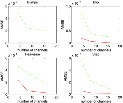
Figure 1: AMSE for the Bumps, Blip, Heavisine and Step functions sampled at a fixed number of $N=128$ points, based on RSNR${}={}$1, as the number of channels $M$ (and hence the sample size $n$) increases. Solid line: BT wavelet estimator; Dash line: TT wavelet estimator.

We used the test functions “Bumps,” “Blip,” “Heavisine” and “Step,” and set $j_{0}=3$. For a fixed value of the (root) signal-to-noise ratio (RSNR${}={}$1), we generated $S=100$ samples of size $n=NM$ from model (86) in order to calculate the average mean-squared error (AMSE) given by

$$S^{-1}\sum_{m=1}^{S}\sum_{i=1}^{N}\bigl{(}\hat{f}_{n}^{m}(t_{i})-f(t_{i})\bigr{)}^{2}\bigg{/}\sum_{i=1}^{N}f^{2}(t_{i}),\qquad t_{i}=i/N.$$

In Figure 1, for a fixed number of data points $N=2^{7}$, we evaluate the AMSE as the number of channels $M$, and hence the sample size $n$, increases for the four signals mentioned above. Obviously, both BT and TT wavelet estimators improve their performances as $n$ increases, and the BT wavelet estimator appears to have smaller AMSE than the TT wavelet estimator in all cases.

Although not reported here, we also evaluated the precision of the suggested BT wavelet estimator for a wide variety of other test functions [see the list of test functions in Appendix I of Antoniadis, Bigot and Sapatinas (2001)] and RSNRs with very good performances. This numerical study confirms that under the multichannel deconvolution model with a boxcar-like blurring function, block thresholding wavelet estimators with equispaced selection of points $u_{l}$, $l=1,2,\ldots,M$, produce quite accurate estimates of $f(\cdot)$.

8 Concluding remarks

We considered the question of whether and when, in the functional deconvolution setting, it is legitimate to replace the real-life discrete deconvolution problem by its continuous idealization. In other words, using the asymptotical minimax framework, we studied whether the continuous model and the discrete model are equivalent for some or any sampling schemes from the viewpoint of convergence rates, over a wider range of Besov balls and for the $L^{2}$-risk. It is worth mentioning that when we talked about convergence rates we referred to the lower bounds which are attainable up to, at most, a logarithmic factor according to Theorems 1 and 2. In the cases when convergence rates in the discrete model depend on the choice of a sampling scheme, we also explored the optimal sampling strategies. The conclusions of our investigation can be summarized as follows.

If Conditions I, I* and II are satisfied, then the convergence rates in the discrete model are independent of the number $M$, and the choice of sampling points $\underline{u}$ and coincide with the convergence rates in the continuous model. In this case, which we call uniform, it is legitimate to replace discrete model (with any selection of sampling points) by continuous model.

If Condition II does not hold, then there exist at least two different sampling schemes in discrete model which deliver two different sets of convergence rates, and at least one of these sampling schemes leads to the convergence rates different from the continuous model. However, if Condition I holds, one can point out the sampling scheme which delivers the fastest convergence rates, namely, sampling entirely at “the best possible” point $u^{*}$. We refer to this case as regular and explore when, under an arbitrary sampling scheme, convergence rates in the discrete model coincide or do not coincide with the convergence rates in the continuous model. The case of sampling at $u^{*}$ is studied as a particular case.

In addition, we consider convergence rates in the discrete model under uniform or pseudo-uniform sampling strategies. Indeed, when a discrete model is replaced by its continuous counterpart, it is implicitly assumed that sampling is carried out at $M$ equidistant points in the interval $[a,b]$. We formulate conditions when this replacement is legitimate and bring examples when the uniform, or a more general pseudo-uniform, sampling may lead to convergence rates which differ from the convergence rates in the continuous model and are lower than when sampling is carried out entirely at the “best possible” point $u^{*}$. Hence, even in the regular case, one should be extremely careful when replacing a discrete model by its continuous counterpart.

Finally, we study the case when Condition I is violated. We referred to this case as irregular. In this case, the convergence rates in the discrete model depend on a sampling strategy, and, in addition, one cannot design a sampling scheme which delivers the highest convergence rates. Since Condition I can be violated in a variety of ways, in the irregular case a general study is very complex. For this reason, we study a particular example of the irregular case, namely, functional deconvolution with a boxcar-like blurring function. This important model occurs, in the problem of estimation of the speed of a wave on a finite interval (Example 3) as well as, a discrete version of it, in signal and image processing (see Section 6). In the case of a boxcar-like kernel, sampling at any one point is, by far, not the best possible choice and delivers lower convergence rates than the continuous model. The best choice for this model is uniform sampling with a large value of $M=M_{n}$. Indeed, if $M=M_{n}\geq c_{0}n^{1/3}$ for some constant $c_{0}>0$, independent of $n$, and the selection points $u_{1},u_{2},\ldots,u_{M}$, are selected to be equispaced, then, according to Theorem 8, the convergence rates in the discrete model with a boxcar-like blurring function coincide with the convergence rates in the continuous model and cannot be improved.

The assumption that $M=M_{n}$ grows at least at a rate of $n^{1/3}$ is very natural in the inverse mathematical physics problems: in fact, if one samples uniformly in the rectangle $[0,1]\times[a,b]$, then $M_{n}\asymp\sqrt{n}$. However, this assumption is hardly natural in a signal processing setting where $M$ corresponds to a number of physical devices, so even if $M=M_{n}\rightarrow\infty$ as $n\rightarrow\infty$, it grows at a very slow rate. For this reason, the question remains: if $M=M_{n}\rightarrow\infty$ at a rate slower than $O(n^{1/3})$ [e.g., $M=M_{n}=c_{3}n^{\upsilon}$, where $0<\upsilon<1/3$, or $M=M_{n}=c_{4}(\ln n)^{\gamma}$, where $\gamma>0$, for some constants $c_{3}>0$ and $c_{4}>0$, independent of $n$], can one select points $u_{l}\in[a,b]$, $l=1,2,\ldots,M$, such that the convergence rates in the discrete model coincide with the corresponding convergence rates obtained in the continuous model? And, if for some such $M=M_{n}$ the convergence rates in the discrete and the continuous models are not the same, what are the best convergence rates that can be attained and the best selection of points $u_{1},u_{2},\ldots,u_{M}$?

The solution of this question, possibly, rests on very nontrivial results in number theory. Recall that De Canditiis and Pensky (2006) showed that, if $M$ is finite, $M\geq 2$, one of the $u_{l}$’s is a BA irrational number, and $u_{1},u_{2},\ldots,u_{M}$ is a BA irrational tuple, then (82) is valid. The constant $C(M)$ in (82) depends on the value of $M$ and the choice of the BA irrational tuple. Let us now elaborate more on this. Note that the numbers $a_{1},a_{2},\ldots,a_{M}$ is a BA irrational tuple [see, e.g., Schmidt (1980), page 42], if, for any integers $p_{1},p_{2},\ldots,p_{M}$ and $q$, there exists constant $B_{M}$ such that

$$\max(|a_{1}q-p_{1}|,|a_{2}q-p_{2}|,\ldots,|a_{M}q-p_{1}|)\geq B_{M}q^{-1/M},$$

where $B_{M}$ is a positive constant that depends only on $M$. Schmidt [(1980), page 43] showed that, for a finite value of $M$, a BA irrational tuple always exists, and proposed an algorithm for constructing it. It is easy to note that $B_{M}\rightarrow 0$ as $M\rightarrow\infty$. The value of $B_{M}$ affects the value of $C(M)$ in (82) and, therefore, the convergence rates in the discrete model.

Unfortunately, we are not aware of any results in number theory on how $B_{M}$ depends on $M$, and we suspect that relevant results may not have yet been derived. However, a partial answer to the above question, showing that $B_{M}\geq C_{0}\exp(-3M\ln M)$, for some $C_{0}>0$, independent of $M$, $q$ and $p_{1},p_{2},\ldots,p_{M}$, and the construction of minimax upper bounds for the $L^{2}$-risk over a wide range of Besov balls, covering the case $M=M_{n}=o((\ln n)^{u})$, where $u\geq 1/2$, have been recently obtained in Pensky and Sapatinas (2009b).

Appendix: Proofs

Recall that the symbol $C$ is used for a generic positive constant, independent of $n$, while the symbol $K$ is used for a generic positive constant, independent of $m$, $n$, $M$ and $u_{1},u_{2},\ldots,u_{M}$, which either of them may take different values at different places. Proof of Theorem 1 The proof of the lower bounds falls into two parts. First, we consider the lower bounds obtained when the worst functions $f$ (i.e., the hardest functions to estimate) are represented by only one term in a wavelet expansion (sparse case), and then when the worst functions $f$ are uniformly spread over the unit interval $T$ (dense case).

In the continuous model, one can always choose $\varepsilon_{n}=1$, so the only difference with Pensky and Sapatinas (2009a) is an extra logarithmic factor. Since the differences for the discrete model are much more significant, we only consider below the proof for the discrete model.

Sparse case. Let the functions $f_{jk}$ be of the form $f_{jk}=\gamma_{j}\psi_{jk}$ and let $f_{0}\equiv 0$. Note that by (3), in order $f_{jk}\in B_{p,q}^{s}(A)$, we need $\gamma_{j}\leq A2^{-js^{\prime}}$. Set $\gamma_{j}=c2^{-js^{\prime}}$, where $c$ is a positive constant such that $c<A$, and apply the following classical lemma on lower bounds:

Lemma 5 ([Härdle et al. (1998), Lemma 10.1])

Let $V$ be a functional space, and let $d(\cdot,\cdot)$ be a distance on $V$. For $f,g\in V$, denote by $\mathchar 259\relax_{n}(f,g)$ the likelihood ratio $\mathchar 259\relax_{n}(f,g)=d{\mathbb{P}}_{X_{n}^{(f)}}/d{\mathbb{P}}_{X_{n}^{(g)}}$, where $d{\mathbb{P}}_{X_{n}^{(h)}}$ is the probability distribution of the process $X_{n}$ when $h$ is true. Let $V$ contain the functions $f_{0},f_{1},\ldots,f_{\aleph}$ such that (a) $d(f_{k},f_{k^{\prime}})\geq\delta>0$ for $k=0,1,\ldots,\aleph$, $k\neq k^{\prime}$; (b) $\aleph\geq\exp(\lambda_{n})$ for some $\lambda_{n}>0$; (c) $\ln\mathchar 259\relax_{n}(f_{0},f_{k})=u_{nk}-v_{nk}$, where $v_{nk}$ are constants and $u_{nk}$ is a random variable such that there exists $\pi_{0}>0$ with ${\mathbb{P}}_{f_{k}}(u_{nk}>0)\geq\pi_{0}$; (d) $\sup_{k}v_{nk}\leq\lambda_{n}$.

Then $\sup_{f\in V}{\mathbb{P}}_{X_{n}^{(f)}}(d(\tilde{f},f)\geq\delta/2)\geq\pi_{0}/2$ for any arbitrary estimator $\tilde{f}$.

Let now $V=\{f_{jk}\dvtx 0\leq k\leq 2^{j}-1\}$ so that $\aleph=2^{j}$. Choose $d(f,g)=\|f-g\|$, where $\|\cdot\|$ is the $L^{2}$-norm on the unit interval $T$. Then $d(f_{jk},f_{jk^{\prime}})=\gamma_{j}=\delta$. Let $v_{nk}=\lambda_{n}=j\ln 2$ and $u_{nk}=\ln\mathchar 259\relax_{n}(f_{0},f_{jk})+j\ln 2$. Now, to apply Lemma 5, we need to show that for some $\pi_{0}>0$, uniformly for all $f_{jk}$, we have ${\mathbb{P}}_{f_{jk}}(u_{nk}>0)={\mathbb{P}}_{f_{jk}}(\ln\mathchar 259\relax_{n}(f_{0},f_{jk})>-j\ln 2)\geq\pi_{0}>0.$

Note that in the case of the discrete model,

$$-\ln\mathchar 259\relax_{n}(f_{0},f_{jk}) = 0.5\sum_{i=1}^{N}\sum_{l=1}^{M}\{[y(u_{l},t_{i})-\gamma_{j}(\psi_{jk}*g)(u_{l},t_{i})]^{2}-y^{2}(u_{l},t_{i})\}$$

$$= v_{jk}-u_{jk},$$

where

$$u_{jk}=\gamma_{j}\sum_{i=1}^{N}\sum_{l=1}^{M}(\psi_{jk}*g)(u_{l},t_{i})\varepsilon_{li},\qquad v_{jk}=0.5\gamma_{j}^{2}\sum_{i=1}^{N}\sum_{l=1}^{M}[(\psi_{jk}*g)(u_{l},t_{i})]^{2}.$$

Observe that, due to ${\mathbb{P}}(\varepsilon_{li}>0)={\mathbb{P}}(\varepsilon_{li}<0)=0.5$, we have ${\mathbb{P}}(u_{jk}>0)=0.5$. By properties of the discrete Fourier transform and taking into account that in the case of Meyer wavelets $|\psi_{mjk}|\leq 2^{-j/2}$ [see, e.g., Johnstone et al. (2004), page 565], we derive that

$$v_{jk}\leq\frac{\gamma_{j}^{2}}{4\pi}\sum_{i=1}^{N}\sum_{l=1}^{M}\sum_{m\in C_{j}}|\psi_{mjk}|^{2}|g_{m}(u_{l})|^{2}\leq\frac{NM\gamma_{j}^{2}}{4\pi 2^{j}}\sum_{m\in C_{j}}M^{-1}\sum_{l=1}^{M}|g_{m}(u_{l})|^{2}\equiv B_{n},$$

where $B_{n}=(4\pi)^{-1}n2^{-j}\gamma_{j}^{2}\sum_{m\in C_{j}}\tau_{1}^{d}(m,\underline{u},M)$.

Let $j=j_{n}$ be such that $B_{n}\leq 0.5j\ln 2$. Then, by applying Lemma 5 and Chebyshev’s inequality, we obtain

$$\inf_{\tilde{f}_{n}}\sup_{f\in B_{p,q}^{s}(A)}{\mathbb{E}}\|\tilde{f}_{n}-f\|^{2} \geq \inf_{\hat{f}_{n}}\sup_{f\in V}\frac{1}{4}\gamma_{j}^{2}{\mathbb{P}}(\|\tilde{f}_{n}-f\|\geq\gamma_{j}/2)$$

$$\geq 0.25\gamma_{j}^{2}\pi_{0}.$$

Thus we just need to choose the smallest possible $j=j_{n}$ satisfying $B_{n}\leq 0.5j\ln 2$, evaluate $\gamma_{j}=c2^{-js^{\prime}}$ and to plug it into (Appendix: Proofs). By direct calculations, we derive, under condition (19), that

$$\sum_{m\in C_{j}}\tau_{1}^{d}(m,\underline{u},M)\leq\cases{K\varepsilon_{n}2^{-j(2\nu-1)}j^{-\lambda},\qquad\mbox{if $\alpha=0$},\cr K\varepsilon_{n}2^{-j(2\nu+\beta-1)}j^{-\lambda}\exp\bigl{(}-\alpha(2\pi/3)^{\beta}2^{j\beta}\bigr{)},\cr\mbox{\hskip 107.0ptif $\alpha>0$}.}$$ (88)

Hence if $\alpha=0$, then $2^{j_{n}}=C({n^{*}}(\ln{n^{*}})^{-(\lambda+1)})^{1/(2s^{\prime}+2\nu)}$, and if $\alpha>0$, then $2^{j_{n}}=C(\ln{n^{*}})^{1/\beta}$. Now, to obtain the lower bound, plug $\gamma_{j}=c2^{-j_{n}s^{\prime}}$ into (Appendix: Proofs)

$$\quad\inf_{\tilde{f}_{n}}\sup_{f\in B_{p,q}^{s}}{\mathbb{E}}\|\tilde{f}_{n}-f\|^{2}\geq\cases{C({n^{*}})^{{2s^{\prime}}/({2s^{\prime}+2\nu})}(\ln{n^{*}})^{{2s^{\prime}(\lambda+1)}/({2s^{\prime}+2\nu})},\cr\hskip 91.0pt\mbox{if $\alpha=0$},\cr C(\ln{n^{*}})^{-{2s^{\prime}}/{\beta}},\qquad\mbox{if $\alpha>0$}.}$$ (89)

Dense case. Let $\eta$ be the vector with components $\eta_{k}=\pm 1$, $k=0,1,\ldots,\break 2^{j}-1$, denote by $\mathchar 260\relax$ the set of all possible vectors $\eta$ and let $f_{j\eta}=\gamma_{j}\sum_{k=0}^{2^{j}-1}\eta_{k}\psi_{jk}$. Let also $\eta^{i}$ be the vector with components $\eta^{i}_{k}=(-1)^{{\mathbb{I}}(i=k)}\eta_{k}$ for $i,k=0,1,\ldots,$$2^{j}-1$. Note that by (3), in order $f_{j\eta}\in B_{p,q}^{s}(A)$, we need $\gamma_{j}\leq A2^{-j(s+1/2)}$. Set $\gamma_{j}=c_{\star}2^{-j(s+1/2)}$, where $c_{\star}$ is a positive constant such that $c_{\star}<A$, and apply the following lemma on lower bounds:

Lemma 6 ([Willer (2005), Lemma 2])

Let $\mathchar 259\relax_{n}(f,g)$ be defined as in Lemma 5, and let $\eta$ and $f_{j\eta}$ be as described above. Suppose that, for some positive constants $\lambda$ and $\pi_{0}$, we have ${\mathbb{P}}_{f_{j\eta}}(-\ln\mathchar 259\relax_{n}(f_{j\eta^{i}},f_{j\eta})\leq\lambda)\geq\pi_{0},$ uniformly for all $f_{j\eta}$ and all $i=0,\ldots,2^{j}-1$. Then, for any arbitrary estimator $\tilde{f}$ and for some constant $L>0$, one has $\max_{\eta\in\mathchar 260\relax}{\mathbb{E}}_{f_{j\eta}}\|\tilde{f}-f_{j\eta}\|\geq L\pi_{0}e^{-\lambda}2^{j/2}\gamma_{j}.$

Since, by Chebychev’s inequality,

$${\mathbb{P}}_{f_{jk}}\bigl{(}\ln\mathchar 259\relax_{n}(f_{j\eta^{i}},f_{j\eta})>-\lambda\bigr{)}\geq 1-{\mathbb{E}}_{f_{jk}}|{\ln\Lambda_{n}}(f_{j\eta^{i}},f_{jk})|/\lambda,$$

we need to show that ${\mathbb{E}}_{f_{j\eta}}|{\ln\mathchar 259\relax_{n}}(f_{j\eta^{i}},f_{j\eta})|\leq\lambda_{1}$, for a sufficiently small constant $\lambda_{1}>0$. Observe that

$$\ln\mathchar 259\relax_{n}(f_{j\eta^{i}},f_{j\eta}) = 0.5\gamma_{j}^{2}\sum_{i=1}^{N}\sum_{l=1}^{M}[(g*f_{j\eta^{i}}-f_{j\eta})(u_{l},t_{i})]^{2}$$

$${}-\gamma_{j}\sum_{i=1}^{N}\sum_{l=1}^{M}\varepsilon_{li}\bigl{[}(g*[f_{j\eta^{i}}-f_{j\eta}])(u_{l},t_{i})\bigr{]}.$$

Then, due to $|f_{j\eta^{i}}-f_{j\eta})|=2|\psi_{jk}|$, one has ${\mathbb{E}}_{f_{j\eta}}|{\ln\mathchar 259\relax_{n}}(f_{j\eta^{i}},f_{j\eta})|\leq A_{n}+B_{n}$ where

$$A_{n} = 2\gamma_{j}{\mathbb{E}}\Biggl{|}\sum_{i=1}^{N}\sum_{l=1}^{M}(\psi_{jk}*g)(u_{l},t_{i})\varepsilon_{li}\Biggr{|},$$

$$B_{n} = 2\gamma_{j}^{2}\sum_{i=1}^{N}\sum_{l=1}^{M}(\psi_{jk}*g)^{2}(u_{l},t_{i}).$$

Since, by Jensen’s inequality, $A_{n}\leq\sqrt{2B_{n}}$, we only need to construct an upper bound for $B_{n}$. Note that, similarly to the sparse case, one has $B_{n}=O(n2^{-j}\gamma_{j}^{2}\sum_{m\in C_{j}}\tau_{1}^{d}(m,\underline{u},M))$. According to Lemma 6, we choose $j=j_{n}$ that satisfies the condition $B_{n}+\sqrt{2B_{n}}\leq\lambda_{1}$. Using (88), we derive that $2^{j_{n}}=C({n^{*}}(\ln{n^{*}})^{-\lambda})^{1/(2s+2\nu+1)}$ if $\alpha=0$ and $2^{j_{n}}=C(\ln{n^{*}})^{1/\beta}$ if $\alpha>0$. Then, Lemma 6 and Jensen’s inequality yield

$$\qquad\inf_{\tilde{f}_{n}}\sup_{f\in B_{p,q}^{s}}{\mathbb{E}}\|\tilde{f}_{n}-f\|^{2}\geq\cases{C({n^{*}})^{-{2s}/({2s+2\nu+1})}(\ln{n^{*}})^{-{2s\lambda}/({2s+2\nu+1})},\cr\hskip 88.8pt\mbox{if $\alpha=0$},\cr C(\ln{n^{*}})^{-{2s}/{\beta}},\qquad\mbox{if $\alpha>0$}.}$$ (90)

Now, to complete the proof one just needs to note that ${s^{*}}=\min(s,s^{\prime})$, and that

$$2s/(2s+2\nu+1)\leq 2s^{*}/(2s^{*}+2\nu)\qquad\mbox{if }\nu(2-p)\leq ps^{*},$$ (91)

with the equalities taken place simultaneously, and then to choose the highest of the lower bounds (89) and (90). This completes the proof of Theorem 1. Proof of Lemma 1 In what follows, we shall only construct the proof for $b_{jk}$ since the proof for $a_{j_{0}k}$ is very similar. Again, we construct the proof only for discrete model, since in the case of continuous model, one can always choose $\varepsilon_{n}=1$, so the only difference with Pensky and Sapatinas (2009a) is an extra logarithmic factor.

Note that, by (11), one has $\hat{b}_{jk}-b_{jk}=\sum_{m\in C_{j}}(\hat{f}_{m}-f_{m})\overline{\psi_{mjk}},$ with

$$\hat{f}_{m}-f_{m}=N^{-1/2}\Biggl{(}\sum_{l=1}^{M}\overline{g_{m}(u_{l})}z_{ml}\Biggr{)}\Bigg{/}\Biggl{(}\sum_{l=1}^{M}|g_{m}(u_{l})|^{2}\Biggr{)},$$ (92)

where $z_{ml}$ are standard (complex-valued) Gaussian random variables, independent for different $m$ and $l$. Therefore,

$${\mathbb{E}}|\hat{b}_{jk}-b_{jk}|^{2}=N^{-1}\sum_{m\in C_{j}}|\psi_{mjk}|^{2}\Biggl{[}\sum_{l=1}^{M}|g_{m}(u_{l})|^{2}\Biggr{]}^{-1}=O(n^{-1}\Delta_{1}(j))$$

since $|C_{j}|=4\pi 2^{j}$ and $|\psi_{mjk}|^{2}\leq 2^{-j}$. If $\kappa=2$, then

$${\mathbb{E}}|\hat{b}_{jk}-b_{jk}|^{4} = O\biggl{(}\sum_{m\in C_{j}}{\mathbb{E}}|\hat{f}_{m}-f_{m}|^{4}|\psi_{mjk}|^{4}\biggr{)}$$

$${}+O\biggl{(}\biggl{[}\sum_{m\in C_{j}}{\mathbb{E}}|\hat{f}_{m}-f_{m}|^{2}|\psi_{mjk}|^{2}\biggr{]}^{2}\biggr{)}$$

$$= O\bigl{(}2^{-j}N^{-2}M^{-3}\Delta_{2}(j)+N^{-2}M^{-2}\Delta_{1}^{2}(j)\bigr{)}$$

$$= O\bigl{(}2^{-j}n^{-2}M^{-1}\Delta_{2}(j)+n^{-2}\Delta_{1}^{2}(j)\bigr{)}.$$

Direct calculations show that when $\alpha=0$ one has $\Delta_{2}(j)=O(2^{6j\nu}j^{3\lambda}\varepsilon_{n}^{-3})$. Plugging expressions for $\Delta_{1}(j)$ and $\Delta_{2}(j)$ into formula (Appendix: Proofs) and taking into account that $2^{j}\leq 2^{J-1}<({n^{*}})^{1/(2\nu+1)}$, one derives

$${\mathbb{E}}|\hat{b}_{jk}-b_{jk}|^{4} = O\biggl{(}\frac{2^{6j\nu}j^{3\lambda}}{n^{2}\varepsilon^{3}M_{n}}+\frac{2^{4j\nu}j^{2\lambda}}{n^{2}\varepsilon^{2}}\biggr{)}$$

$$= O\bigl{(}n({n^{*}})^{{6\nu}/({2\nu+1})-3}(\ln n)^{3\lambda}+({n^{*}})^{{4\nu}/({2\nu+1})-2}(\ln n)^{2\lambda}\bigr{)}.$$

To complete the proof, observe that in the last expression, the second term is asymptotically smaller than the first. Proof of Lemma 2 Again we carry out the proof only for the discrete case. The proof for the continuous case can be obtained as a minor variation of the proof below. Consider the set of vectors $\mathchar 266\relax_{jr}=\{v_{k},k\in U_{jr}\dvtx\sum_{k\in U_{jr}}|v_{k}|^{2}\leq 1\}$ and the centered Gaussian process defined by $Z_{jr}(v)=\sum_{k\in U_{jr}}v_{k}(\hat{b}_{jk}-b_{jk}).$ The proof of the lemma is based on the following inequality:

Lemma 7 ([Cirelson, Ibragimov and Sudakov (1976)])

Let $D$ be a subset of $\mathbb{R}=(-\infty,\infty)$, and let $(\xi_{t})_{t\in D}$ be a centered Gaussian process. If ${\mathbb{E}}(\sup_{t\in D}\xi_{t})\leq B_{1}$ and $\sup_{t\in D}\operatorname{Var}(\xi_{t})\leq B_{2}$, then, for all $x>0$, we have ${\mathbb{P}}(\sup_{t\in D}\xi_{t}\geq x+B_{1})\leq\exp(-x^{2}/(2B_{2})).$

To apply Lemma 7, we need to find $B_{1}$ and $B_{2}$. Note that, by Jensen’s inequality, we obtain

$${\mathbb{E}}\Bigl{[}\sup_{v\in\mathchar 266\relax_{jr}}Z_{jr}(v)\Bigr{]} = {\mathbb{E}}\biggl{[}\sum_{k\in U_{jr}}|\hat{b}_{jk}-b_{jk}|^{2}\biggr{]}^{1/2}\leq\biggl{[}\sum_{k\in U_{jr}}{\mathbb{E}}|\hat{b}_{jk}-b_{jk}|^{2}\biggr{]}^{1/2}$$

$$\leq \frac{\sqrt{c_{1}}2^{\nu j}j^{\lambda/2}\sqrt{\ln n}}{\sqrt{{n^{*}}}}=B_{1}.$$

[Here $c_{1}$ is the same positive constant as in (29) with $\alpha=0$.] Also, by (4) and (92), we have ${\mathbb{E}}[(\hat{b}_{jk}-b_{jk})(\hat{b}_{jk^{\prime}}-b_{jk^{\prime}})]=n^{-1}\sum_{m\in C_{j}}\psi_{mjk}\overline{\psi_{mjk^{\prime}}}[\tau_{1}(m)]^{-1}$ where $\tau_{1}(m)$ is defined in (18). Hence

$$\sup_{v\in\mathchar 266\relax_{jr}}\operatorname{Var}(Z_{jr}(v)) = n^{-1}\sup_{v\in\mathchar 266\relax_{jr}}\sum_{k\in U_{jr}}\sum_{k^{\prime}\in U_{jr}}v_{k}v_{k^{\prime}}\sum_{m\in C_{j}}\psi_{mjk}\overline{\psi_{mjk^{\prime}}}[\tau_{1}(m)]^{-1}$$

$$\leq c_{1}({n^{*}})^{-1}2^{2\nu j}j^{\lambda}\sum_{k\in U_{jr}}v^{2}_{k}\leq c_{1}({n^{*}})^{-1}2^{2\nu j}j^{\lambda}=B_{2},$$

by using $\sum_{m\in C_{j}}\psi_{mjk}\overline{\psi_{mjk^{\prime}}}={\mathbb{I}}(k=k^{\prime})$ and (29) for $\alpha=0$. Therefore, by applying Lemma 7 with $B_{1}$ and $B_{2}$ defined above and $x=B_{1}((2\sqrt{c_{1}})^{-1}\mu\sqrt{h_{2}}-1),$ and noting that under condition (32), $\ln({n^{*}})\geq h_{2}\ln n$, we derive

$${\mathbb{P}}\biggl{(}\sum_{k\in U_{jr}}|\hat{b}_{jk}-b_{jk}|^{2}\geq\frac{\mu^{2}2^{2\nu j}j^{\lambda}\ln({n^{*}})}{4{n^{*}}}\biggr{)}\leq\exp\biggl{\{}-\biggl{(}\frac{\mu\sqrt{h_{2}}}{2\sqrt{c_{1}}}-1\biggr{)}^{2}\frac{B_{1}^{2}}{2B_{2}}\biggr{\}}\leq n^{-3},$$

since (32) implies that $0.5[\mu\sqrt{h_{2}}/(2\sqrt{c_{1}})-1]^{2}\geq 3$. This completes the proof of Lemma 2. Proof of Theorem 2 First, note that in the case of $\alpha>0$, we have ${\mathbb{E}}\|\hat{f}_{n}-f\|^{2}=R_{1}+R_{2}$, where

$$R_{1}=\sum_{j=J}^{\infty}\sum_{k=0}^{2^{j}-1}b_{jk}^{2},\qquad R_{2}=\sum_{k=0}^{2^{j_{0}}-1}{\mathbb{E}}(\hat{a}_{j_{0}k}-a_{j_{0}k})^{2},$$ (94)

since ${j_{0}}=J$. It is well known [see, e.g., Johnstone (2002), Lemma 19.1] that if $f\in B_{p,q}^{s}(A)$, then for some positive constant $c^{\star}$, dependent on $p$, $q$, $s$ and $A$ only, we have

$$\sum_{k=0}^{2^{j}-1}b_{jk}^{2}\leq c^{\star}2^{-2j{s^{*}}};$$ (95)

thus $R_{1}=O(2^{-2J{s^{*}}})=O((\ln{n^{*}})^{-2{s^{*}}/\beta})$. Also, using (29) and (30), we derive $R_{2}=O(n^{-1}2^{j_{0}}\Delta_{1}({j_{0}}))=O(({n^{*}})^{-1/2}(\ln{n^{*}})^{2\nu/\beta})=o((\ln{n^{*}})^{-2{s^{*}}/\beta}),$ thus completing the proof for $\alpha>0$.

Now consider the case of $\alpha=0$. Note that by condition (23) one has $\ln{n^{*}}\asymp\ln n$. Due to the orthonormality of the wavelet basis, we obtain

$${\mathbb{E}}\|\hat{f}_{n}-f\|^{2}=R_{1}+R_{2}+R_{3}+R_{4},$$ (96)

where $R_{1}$ and $R_{2}$ are defined in (94), and

$$R_{3} = \sum_{j=j_{0}}^{J-1}\sum_{r\in A_{j}}\sum_{k\in U_{jr}}{\mathbb{E}}\bigl{[}(\hat{b}_{jk}-b_{jk})^{2}{\mathbb{I}}\bigl{(}\hat{B}_{jr}\geq\mu^{2}({n^{*}})^{-1}2^{2\nu j}\ln({n^{*}})j^{\lambda}\bigr{)}\bigr{]},$$

$$R_{4} = \sum_{j=j_{0}}^{J-1}\sum_{r\in A_{j}}\sum_{k\in U_{jr}}{\mathbb{E}}\bigl{[}b_{jk}^{2}{\mathbb{I}}\bigl{(}\hat{B}_{jr}<\mu^{2}({n^{*}})^{-1}2^{2\nu j}\ln({n^{*}})j^{\lambda}\bigr{)}\bigr{]},$$

where $\hat{B}_{jr}$ and $\mu$ are defined by (12), (26) and (32), respectively.

Let us now examine each term in (96) separately. Similarly to the case of $\alpha>0$, we obtain $R_{1}=O(2^{-2J{s^{*}}})=O(n^{-2{s^{*}}/(2\nu+1)})$. By direct calculations, one can check that $2{s^{*}}/(2\nu+1)>2s/(2s+2\nu+1)$, if $\nu(2-p)<p{s^{*}}$, and $2{s^{*}}/(2\nu+1)\geq 2{s^{*}}/(2{s^{*}}+2\nu)$, if $\nu(2-p)\geq p{s^{*}}$. Hence

$$R_{1}=\cases{O\bigl{(}({n^{*}})^{-{2s}/({2s+2\nu+1})}\bigr{)},&\quad if $\nu(2-p)<p{s^{*}}$,\cr O\bigl{(}({n^{*}})^{-{2{s^{*}}}/({2{s^{*}}+2\nu})}\bigr{)},&\quad if $\nu(2-p)\geq p{s^{*}}$.}$$ (97)

Also, by (30) and (29), we obtain

$$R_{2} = O\bigl{(}({n^{*}})^{-1}2^{(2\nu+1){j_{0}}}\bigr{)}=o\bigl{(}({n^{*}})^{-{2s}/({2s+2\nu+1})}\bigr{)}$$

$$= o\bigl{(}({n^{*}})^{-{2s^{*}}/({2s^{*}+2\nu})}\bigr{)}.$$

Denote

$$\Theta_{jr}=\biggl{\{}\omega\dvtx\sum_{k\in U_{jr}}|\hat{b}_{jk}-b_{jk}|^{2}\geq 0.25\mu^{2}({n^{*}})^{-1}2^{2\nu j}\ln({n^{*}})j^{\lambda}\biggr{\}}.$$

To construct the upper bounds for $R_{3}$ and $R_{4}$, note that simple algebra yields $R_{3}\leq(R_{31}+R_{32}),R_{4}\leq(R_{41}+R_{42}),$ where

$$R_{31} = \sum_{j=j_{0}}^{J-1}\sum_{r\in A_{j}}\sum_{k\in U_{jr}}{\mathbb{E}}[(\hat{b}_{jk}-b_{jk})^{2}{\mathbb{I}}(\Theta_{jr})],$$

$$R_{41} = \sum_{j=j_{0}}^{J-1}\sum_{r\in A_{j}}\sum_{k\in U_{jr}}{\mathbb{E}}[b_{jk}^{2}{\mathbb{I}}(\Theta_{jr})],$$

$$R_{32} = \sum_{j=j_{0}}^{J-1}\sum_{r\in A_{j}}\sum_{k\in U_{jr}}{\mathbb{E}}\bigl{[}(\hat{b}_{jk}-b_{jk})^{2}{\mathbb{I}}\bigl{(}B_{jr}>0.25\mu^{2}({n^{*}})^{-1}2^{2\nu j}\ln({n^{*}})j^{\lambda}\bigr{)}\bigr{]},$$

$$R_{42} = \sum_{j=j_{0}}^{J-1}\sum_{r\in A_{j}}\sum_{k\in U_{jr}}{\mathbb{E}}\bigl{[}b_{jk}^{2}{\mathbb{I}}\bigl{(}B_{jr}<2.5\mu^{2}({n^{*}})^{-1}2^{2\nu j}\ln({n^{*}})j^{\lambda}\bigr{)}\bigr{]}.$$

Then, by (95), Lemmas 1 and 2, and the Cauchy–Schwarz inequality, we derive

$$R_{31}+R_{41} = O\Biggl{(}\sum_{j=j_{0}}^{J-1}\sum_{r\in A_{j}}\sum_{k\in U_{jr}}\bigl{[}\sqrt{{\mathbb{E}}(\hat{b}_{jk}-b_{jk})^{4}}+b_{jk}^{2}\bigr{]}\sqrt{{\mathbb{P}}(\Theta_{jr})}\Biggr{)}$$

$$= O\Biggl{(}\sum_{j=j_{0}}^{J-1}\bigl{[}\sqrt{n}(\ln n)^{3\lambda/2}({n^{*}})^{-{3}/({2(2\nu+1)})}+2^{-2j{s^{*}}}\bigr{]}n^{-{3/2}}\Biggr{)}$$

$$= O(({n^{*}})^{-1}),$$

provided $\mu$ satisfies (32). Hence

$$\mathchar 257\relax_{1}=R_{31}+R_{41}=O(({n^{*}})^{-1}).$$ (99)

Now, consider

$$\mathchar 257\relax_{2}=R_{32}+R_{42}.$$ (100)

First, let us study the dense case, that is, when $\nu(2-p)<p{s^{*}}$. Let $j_{1}$ be such that

$$2^{j_{1}}=({n^{*}})^{{1}/({2s+2\nu+1})}(\ln n)^{({(2/p-1)_{+}-\lambda})/({2\nu+2s+1})}.$$ (101)

Then, $\mathchar 257\relax_{2}$ can be partitioned as $\mathchar 257\relax_{2}=\mathchar 257\relax_{21}+\mathchar 257\relax_{22}$, where the first component is calculated over the set of indices ${j_{0}}\leq j\leq j_{1}$ and the second component over $j_{1}+1\leq j\leq J-1$. Hence, using (12) and Lemma 1, and taking into account that the cardinality of $A_{j}$ is $|A_{j}|=2^{j}/\ln n$, we obtain

$$\mathchar 257\relax_{21} = O\Biggl{(}\sum_{j=j_{0}}^{j_{1}}\Biggl{[}\frac{2^{(2\nu+1)j}j^{\lambda}}{{n^{*}}}+\sum_{r\in A_{j}}\frac{2^{2\nu j}\ln({n^{*}})j^{\lambda}}{{n^{*}}}\Biggr{]}\Biggr{)}$$

$$= O\Biggl{(}\Biggl{[}\frac{(\ln n)^{\lambda}}{{n^{*}}}\Biggr{]}^{{2s}/({2s+2\nu+1})}(\ln n)^{\varrho}\Biggr{)},$$

where $\varrho$ is defined in (27). To obtain an expression for $\mathchar 257\relax_{22}$, note that for $p\geq 2$, by (23) and (95), we have

$$\mathchar 257\relax_{22} = O\Biggl{(}\sum_{j=j_{1}+1}^{J-1}\sum_{r\in A_{j}}B_{jr}\Biggr{)}=O\Biggl{(}\sum_{j=j_{1}+1}^{J-1}2^{-2js}\Biggr{)}$$

$$= O\bigl{(}({n^{*}})^{-{2s}/({2s+2\nu+1})}(\ln n)^{{2s\lambda}/({2s+2\nu+1})}\bigr{)}.$$

If $1\leq p<2$, then $B_{jr}^{p/2}=(\sum_{k\in U_{jr}}b_{jk}^{2})^{p/2}\leq\sum_{k\in U_{jr}}|b_{jk}|^{p},$ so that by Lemma 1, and since $\nu(2-p)<ps^{*}$, we obtain

$$\mathchar 257\relax_{22} = O\Biggl{(}\sum_{j=j_{1}+1}^{J-1}\sum_{r\in A_{j}}[(({n^{*}})^{-1}2^{2\nu j}j^{\lambda}\ln n)^{1-p/2}B_{jr}^{p/2}]\Biggr{)}$$

$$= O\Biggl{(}\sum_{j=j_{1}+1}^{J-1}(({n^{*}})^{-1}2^{2\nu j}j^{\lambda}\ln n)^{1-p/2}2^{-pjs^{*}}\Biggr{)}$$

$$= O\bigl{(}({n^{*}})^{-{2s}/({2s+2\nu+1})}(\ln n)^{{2s\lambda}/({2s+2\nu+1})+\varrho}\bigr{)}.$$

Let us now study the sparse case when $\nu(2-p)>p{s^{*}}$. Let $j_{1}$ be defined by $2^{j_{1}}=({n^{*}})^{{1}/({2s+2\nu+1})}(\ln n)^{{-\lambda}/({2\nu+2s+1})}$. Hence, if $B_{jr}\geq 0.25\mu^{2}({n^{*}})^{-1}2^{2\nu j}\times\break\ln({n^{*}})j^{\lambda}$, then $B_{jr}\leq\sum_{k=0}^{2^{j}-1}b_{jk}^{2}\leq c^{*}2^{-2j{s^{*}}}$ [see (95)] implies that $j\leq j_{2}$ where $j_{2}$ is such that $2^{j_{2}}=C[{n^{*}}/(\ln n)^{1+\lambda}]^{1/(2{s^{*}}+2\nu)}$, where $C$ depends on $\mu$ and $c^{*}$ only. Again, partition $\mathchar 257\relax_{2}=\mathchar 257\relax_{21}+\mathchar 257\relax_{22}$, where the first component is calculated over ${j_{0}}\leq j\leq j_{2}$ and the second component over $j_{2}+1\leq j\leq J-1$. Then, using similar arguments to that in (Appendix: Proofs), and taking into account that $\nu(2-p)>p{s^{*}}$, we derive

$$\mathchar 257\relax_{21} = O\Biggl{(}\sum_{j=j_{0}}^{j_{2}}[({n^{*}})^{-1}2^{2\nu j}j^{\lambda}\ln n]^{1-p/2}\sum_{r\in A_{j}}\sum_{k\in U_{jr}}|b_{jk}|^{p}\Biggr{)}$$

$$= O\Biggl{(}\sum_{j=j_{0}}^{j_{2}}[({n^{*}})^{-1}2^{2\nu j}j^{\lambda}\ln n]^{1-p/2}2^{-pj{s^{*}}}\Biggr{)}$$

$$= O\bigl{(}[({n^{*}})^{-1}(\ln n)^{1+\lambda}]^{{2{s^{*}}}/({2s^{*}+2\nu})}\bigr{)}.$$

To obtain an upper bound for $\mathchar 257\relax_{22}$, recall (100) and keep in mind that the portion of $R_{32}$ corresponding to $j_{2}+1\leq j\leq J-1$ is just zero. Hence, by (95), we obtain

$$\mathchar 257\relax_{22} = O\Biggl{(}\sum_{j=j_{2}+1}^{J-1}\sum_{k=0}^{2^{j}-1}b_{jk}^{2}\Biggr{)}=O\Biggl{(}\sum_{j=j_{2}+1}^{J-1}2^{-2j{s^{*}}}\Biggr{)}$$

$$= O\bigl{(}[({n^{*}})^{-1}(\ln n)^{1+\lambda}]^{{2{s^{*}}}/({2s^{*}+2\nu})}\bigr{)}.$$

Now, in order to complete the proof, we just need to study the case when $\nu(2-p)=p{s^{*}}$. In this situation, we have $2s/(2s+2\nu+1)=2s^{*}/(2s^{*}+2\nu)=1-p/2$ and $2\nu j(1-p/2)=pjs^{*}$. Recalling (3) and noting that $s^{*}\leq s^{\prime}$, we obtain $\sum_{j=j_{0}}^{J-1}(2^{pjs^{*}}\sum_{k=0}^{2^{j}-1}|b_{jk}|^{p})^{q/p}\leq A^{q}.$ Then we repeat the calculations in (Appendix: Proofs) for all indices ${j_{0}}\leq j\leq J-1$. If $1\leq p<q$, then, by Hölder’s inequality, we obtain

$$\mathchar 257\relax_{2} = O\Biggl{(}(({n^{*}})^{-1}(\ln n)^{1+\lambda})^{1-p/2}(\ln n)^{1-p/q}$$

$$\hskip 14.2pt{}\times\Biggl{[}\sum_{j=j_{0}}^{J-1}\Biggl{(}2^{pjs^{*}}\sum_{k=0}^{2^{j}-1}|b_{jk}|^{p}\Biggr{)}^{q/p}\Biggr{]}^{p/q}\Biggr{)}$$

$$= O\bigl{(}(({n^{*}})^{-1}(\ln n)^{1+\lambda})^{{2{s^{*}}}/({2s^{*}+2\nu})}(\ln n)^{1-p/q}\bigr{)}.$$

If $1\leq q\leq p$, then, by the inclusion $B_{p,q}^{s}(A)\subset B_{p,p}^{s}(A)$, we obtain

$$\mathchar 257\relax_{2} = O\Biggl{(}\sum_{j=j_{0}}^{J-1}\bigl{(}(\ln n)^{1+\lambda}/{n^{*}}\bigr{)}^{1-p/2}2^{pjs^{*}}\sum_{k=0}^{2^{j}-1}|b_{jk}|^{p}\Biggr{)}$$

$$= O\bigl{(}\bigl{(}(\ln n)^{1+\lambda}/{n^{*}}\bigr{)}^{{2{s^{*}}}/({2s^{*}+2\nu})}\bigr{)}.$$

By combining (97), (Appendix: Proofs), (99), (Appendix: Proofs)–(Appendix: Proofs), we complete the proof of Theorem 2. Proof of Theorem 3 The first part of the theorem is identical to Proposition 1 of Pensky and Sapatinas (2009a). The second part can be proved by contradiction. Assume that, assumptions (36) and (37) hold but condition (38) does not take place. It follows from (36) and (37) that

$$|g_{m}(u_{*})|^{2} \leq K|m|^{-2\nu_{1}}\exp(-\alpha_{1}|m|^{\beta_{1}}),\qquad\nu_{1}>0\mbox{ if }\alpha_{1}=0,$$

$$|g_{m}(u^{*})|^{2} \geq K|m|^{-2\nu_{2}}\exp(-\alpha_{2}|m|^{\beta_{2}}),\qquad\nu_{2}>0\mbox{ if }\alpha_{2}=0.$$

Observe that condition (38) of Theorem 3 can be violated only in one of the following ways: $\alpha_{1}=\alpha_{2}=0$ but $\nu_{2}<\nu_{1}$, or $\alpha_{1}>0$ but $\alpha_{2}=0$, or $\alpha_{1}>0$ and $\alpha_{2}>0$ but $\beta_{2}<\beta_{1}$.

Applying Theorem 1 with $M=1$, $\varepsilon_{n}=1$ and $u_{1}=u_{*}$, we arrive at, as $n\rightarrow\infty$,

$$R_{n}^{d}(B_{p,q}^{s}(A),u_{*},1)\geq\cases{Cn^{-{2s}/({2s+2\nu_{1}+1})},&\quad if $\alpha_{1}=0,\nu_{1}(2-p)<p{s^{*}}$,\cr C\biggl{(}\dfrac{\ln n}{n}\biggr{)}^{{2{s^{*}}}/({2s^{*}+2\nu_{1}})},&\quad if $\alpha_{1}=0,\nu_{1}(2-p)\geq p{s^{*}}$,\cr C(\ln n)^{-{2{s^{*}}}/{\beta_{1}}},&\quad if $\alpha_{1}>0$.}$$

On the other hand, applying Theorem 2 with $M=1$, $\varepsilon_{n}=1$ and $u_{1}=u^{*}$, we derive that, as $n\rightarrow\infty$,

$$\sup_{f\in B_{p,q}^{s}(A)}{\mathbb{E}}\|\hat{f}_{n}^{d}-f\|^{2}\leq\cases{Cn^{-{2s}/({2s+2\nu_{2}+1})}(\ln n)^{\varrho},\cr\hskip 91.0pt\mbox{if $\alpha_{2}=0,\nu_{2}(2-p)<p{s^{*}}$},\cr C\biggl{(}\dfrac{\ln n}{n}\biggr{)}^{{2{s^{*}}}/({2s^{*}+2\nu_{2}})}(\ln n)^{\varrho},\cr\hskip 91.0pt\mbox{if $\alpha_{2}=0,\nu_{2}(2-p)\geq p{s^{*}}$},\cr C(\ln n)^{-{2{s^{*}}}/{\beta_{2}}},\qquad\mbox{if $\alpha_{2}>0$},}$$

where $\rho$ is given by formula (27) with $\nu=\nu_{2}$. Now, to complete the proof just note that if $\alpha_{1}=\alpha_{2}=0$ but $\nu_{2}<\nu_{1}$ or $\alpha_{1}>0$ but $\alpha_{2}=0$ or $\alpha_{1}\alpha_{2}>0$ but $\beta_{2}<\beta_{1}$, then the asymptotical minimax lower bounds for the $L^{2}$-risk at the point $u=u_{*}$ are higher than the corresponding upper bounds at the point $u=u^{*}$. Hence, in this case, the convergence rates cannot be independent of the choice of $M$ and the selection of points $\underline{u}$, arriving at the required contradiction. Proof of Theorem 4 Note that the first inequality in formula (45), as well as relations (46) and (47) between upper bounds in discrete and continuous cases, follow directly from Theorems 1 and 2 and from inequalities $\tau_{1}^{d}(m,u^{*},1)\geq K\tau_{1}^{c}(m)$ and $\tau_{1}^{d}(m,u^{*},1)\geq K\tau_{1}^{d}(m,\underline{u},M)$. Hence one only needs to prove the second asymptotic relation in formula (45).

Let $R_{n}^{d}(B_{p,q}^{s}(A),\underline{u},M)$ be the minimax $L^{2}$-risk for fixed values of $\underline{u}$ and $M$, defined by formula (16), and let

$$H(\underline{u},M,j)=2^{-j}\gamma_{j}^{2}\sum_{m\in C_{j}}\tau_{1}^{d}(m,\underline{u},M).$$

From the proof of Theorem 1 of Pensky and Sapatinas (2009a), it follows that, in the sparse case [when $\nu(2-p)\geq p{s^{*}}$], one has $R_{n}^{d}(B_{p,q}^{s}(A),\underline{u},M)\geq C2^{-2{j_{n}}{s^{*}}}$, as $n\rightarrow\infty$, where ${j_{n}}\equiv{j_{n}}(\underline{u},M)$ is such that $nH(\underline{u},M,j_{n})/{j_{n}}=C$. Similarly, in the dense case [when $\nu(2-p)<p{s^{*}}$], one has $R_{n}^{d}(B_{p,q}^{s}(A),\underline{u},M)\geq C2^{-2{j_{n}}s}$, as $n\rightarrow\infty$, where ${j_{n}}\equiv{j_{n}}(\underline{u},M)$ is such that $nH(\underline{u},M,j_{n})=C$.

Consider now two different values of $M$, say $M_{1}$ and $M_{2}$, and the corresponding sets of $\underline{u}$’s, say $\underline{u}_{1}$ and $\underline{u}_{2}$. If $\tau_{1}^{d}(m,\underline{u}_{1},M_{1})<\tau_{1}^{d}(m,\underline{u}_{2},M_{2})$ for any $m\in C_{j}$, then $H(\underline{u}_{1},M_{1},j)<H(\underline{u}_{2},M_{2},j)$. Observe that, for fixed $M$ and $\underline{u}$, both $H(\underline{u},M,j)$ and $H(\underline{u},M,j)/j$ are decreasing functions of $j$. Hence, if $j_{n1}={j_{n}}(\underline{u}_{1},M_{1})$ and $j_{n2}={j_{n}}(\underline{u}_{2},M_{2})$ are the values of ${j_{n}}$ corresponding to $(\underline{u}_{1},M_{1})$ and $(\underline{u}_{2},M_{2})$, respectively, then $j_{n1}\leq j_{n2}$. To show that this is true in the dense case, observe that the opposite, $j_{n1}>j_{n2}$, implies $Cn^{-1}=H(\underline{u}_{1},M_{1},j_{n1})<H(\underline{u}_{1},M_{1},j_{n2})<H(\underline{u}_{2},M_{2},j_{n2}),$ so that $j_{n2}$ cannot be the solution of equation $H(\underline{u}_{2},M_{2},j_{n2})=Cn^{-1}$ and $j_{n1}>j_{n2}$ cannot be true. In the sparse case, one just needs to replace $H(\underline{u},M,j)$ by $H(\underline{u},M,j)/j$.

Now, it follows immediately that in both sparse and dense cases, $R_{n}^{d}(B_{p,q}^{s}(A)$, $\underline{u}_{1},M_{1})>R_{n}^{d}(B_{p,q}^{s}(A),\underline{u}_{2},M_{2})$. Therefore, the infimum of $R_{n}^{d}(B_{p,q}^{s}(A),\underline{u},M)$ is attained at $\tilde{M}$ and $\tilde{\underline{u}}$ such that $\tau_{1}^{d}(m,\tilde{\underline{u}},\tilde{M})=\sup_{\underline{u},M}\tau_{1}^{d}(m,\underline{u},M)$. Since, for any choice of $M$ and any selection of points $\underline{u}$, one has $\tau_{1}^{d}(m,\underline{u},M)\leq K\tau_{1}^{d}(m;u^{*},1)$, the validity of the theorem follows from Theorem 1 in Pensky and Sapatinas (2009a). Proof of Lemma 3 Recall that $\tau_{1}^{c}(m)=\int_{a}^{b}|g_{m}(u)|^{2}\,du$ and $\tau_{1}^{d}(m,u^{*},1)=|g_{m}(u^{*})|^{2}$. Observe that since $\nu(\cdot)$, $\alpha(\cdot)$ and $\beta(\cdot)$ are continuous functions on the interval $U=[a,b]$, then there exist $\nu_{1}\leq\nu_{2}$, $\alpha_{1}\leq\alpha_{2}$ and $\beta_{1}\leq\beta_{2}$ such that $\nu_{1}\leq\nu(u)\leq\nu_{2}$, $\alpha_{1}\leq\alpha(u)\leq\alpha_{2}$ and $\beta_{1}\leq\beta(u)\leq\beta_{2}$, $u\in[a,b]$. Moreover, in the inequalities above, either $\alpha_{1}=\alpha_{2}=0$ and $\nu_{1}>0$, or $\alpha_{1}>0$ and $\beta_{1}>0$. Consider the cases when (a) $\alpha(u)\equiv 0$ and (b) $\alpha(u)>0$, $\beta(u)\neq\mbox{const}$.

Case 1: $\alpha(u)\equiv 0$. Then $|g_{m}(u)|^{2}\asymp|m|^{-2\nu(u)}$, so that $|g_{m}(u)|^{2}\leq K|g_{m}(u^{*})|^{2}$ and $|g_{m}(u^{*})|^{2}\asymp|m|^{-2\nu(u^{*})}$. Hence, in the discrete case, the asymptotical minimax lower bounds in (5.3) and the asymptotical minimax upper bounds in (5.3), for the $L^{2}$-risk, follow directly from Theorems 1 and 2, respectively.

In order to complete the proof, we need to obtain the asymptotical minimax lower and upper bounds for the $L^{2}$-risk in the continuous model. For this purpose, observe that, under conditions (52) and (54), one has [see, e.g., Bender and Orzag (1978), pages 266–267]

$$\tau_{1}^{c}(m)\asymp\int_{a}^{b}\exp(-2|{\ln m}|\nu(u))\,du\asymp|m|^{-2\nu(u^{*})}({\ln}|m|)^{-1/k},$$ (108)

so that Theorems 1 and 2 yield, respectively, the asymptotical minimax lower bounds in (3) and the asymptotical minimax upper bounds in (3), for the $L^{2}$-risk.

Case 2: $\alpha(u)>0$ and $\beta(u)\neq\mbox{const}$. In this case, $\beta(u^{*})=\beta_{1}$. Therefore, one derives $K|m|^{-2\nu_{2}}\exp(-\alpha_{2}|m|^{\beta_{1}})\leq|g_{m}(u^{*})|^{2}\leq K|m|^{-2\nu_{1}}\exp(-\alpha_{1}|m|^{\beta_{1}}).$ Hence the asymptotical minimax lower bounds in (5.3) and the asymptotical minimax upper bounds in (5.3), for the $L^{2}$-risk, follow directly from Theorems 1 and 2, respectively.

To obtain the asymptotical minimax lower and upper bounds for the $L^{2}$-risk in the continuous model, note that

$$\tau_{1}^{c}(m) \leq K|m|^{-2\nu_{1}}\int_{a}^{b}\exp\bigl{(}-\alpha(u)|m|^{\beta(u)}\bigr{)}\,du$$

$$\leq C_{3}(b-a)|m|^{-2\nu_{1}}\exp(-\alpha_{1}|m|^{\beta_{1}}).$$

On the other hand,

$$\tau_{1}^{c}(m)\geq K|m|^{-2\nu_{2}}\int_{a}^{b}\exp\bigl{(}-\alpha(u)|m|^{\beta(u)}\bigr{)}\,du.$$ (110)

Since $\beta(\cdot)$ is a continuously differentiable function in some neighborhood of $u^{*}$, $|u-u^{*}|<d$, we have $\beta(u)\leq\beta(u^{*})+\beta_{*}|u-u^{*}|$, where $\beta^{*}={\max_{|u-u^{*}|<d}}|\beta^{\prime}(u)|$. Therefore, using the inequality $e^{z}<1+3z$ for $0<z<1$, we obtain $|m|^{\beta(u)}\leq|m|^{\beta_{1}}\exp(\beta_{*}|u-u^{*}|{\ln}|m|)\leq|m|^{\beta_{1}}(1+3\beta_{*}|u-u^{*}|{\ln}|m|)$ for $|u-u^{*}|<{\ln}|m|/\break(3\beta_{*})$. Denote $\Omega_{m}(u^{*})=\{u\in U\dvtx|u-u^{*}|<|m|^{-(\beta_{1}+1)}\}$. Then

$$\int_{a}^{b}\exp\bigl{(}-\alpha(u)|m|^{\beta(u)}\bigr{)}\,du$$

$$\qquad\geq e^{-\alpha_{2}|m|^{\beta_{1}}}\int_{\Omega_{m}(u^{*})}\exp(-\alpha_{2}|m|^{\beta_{1}}3\beta_{*}|u-u^{*}|{\ln}|m|)\,du$$ (111)

$$\qquad\geq e^{-1}|m|^{-(\beta_{1}+1)}\exp(-\alpha_{2}|m|^{\beta_{1}}),$$

since ${3\beta_{*}\alpha_{2}|m|^{-1}\ln}|m|<1$ for $|m|$ large enough. Combining (Appendix: Proofs)–(Appendix: Proofs), we derive that

$$Ke^{-1}|m|^{-(2\nu_{2}+\beta_{1}+1)}\exp(-\alpha_{2}|m|^{\beta_{1}})$$

(112)

$$\qquad\leq\tau_{1}^{c}(m)\leq K(b-a)|m|^{-2\nu_{1}}\exp(-\alpha_{1}|m|^{\beta_{1}}),$$

so that Theorems 1 and 2 yield, respectively, the asymptotical minimax lower bounds in (3) and the asymptotical minimax upper bounds in (3), for the $L^{2}$-risk. Proof of Theorem 5 First consider the case when $\alpha(u)\equiv 0$. From (52), it follows that $\tau_{1}^{d}(m,\underline{u},M_{n})\leq K|m|^{-2\nu(u^{*})},$ so that $\varepsilon_{n}\leq K({\ln}|m|)^{\lambda_{1}}$. Since, in this case, ${\ln}|m|\asymp\ln n$ and ${\ln}|m|>1$ as $n\rightarrow\infty$, one has $\varepsilon_{n}=O((\ln n)^{\lambda_{3}})$, where $\lambda_{3}=\max(\lambda_{1},0)$. The latter, in combination with (58), implies that condition (23) holds and, moreover, that $Cn(\ln n)^{-\lambda_{2}}\leq{n^{*}}\leq Cn(\ln n)^{\lambda_{3}}$. Then Theorems 1 and 2 imply that under conditions (52), (57) and (58), one has $R_{n}^{d}(B_{p,q}^{s}(A),\underline{u},M)\geq R_{n}^{d}(B_{p,q}^{s}(A))$, where $R_{n}^{d}(B_{p,q}^{s}(A))$ is given by expression (5.3) and that, as $n\rightarrow\infty$,

$$\sup_{f\in B_{p,q}^{s}(A)}{\mathbb{E}}\|\hat{f}_{n}^{d}-f\|^{2}\leq\cases{C(n^{-1}(\ln n)^{\lambda_{1}+\lambda_{2}})^{-{2s}/({2s+2\nu(u^{*})+1})}(\ln n)^{\varrho},\vspace*{2pt}\cr\qquad\mbox{if $\nu(u^{*})(2-p)<p{s^{*}}$},\vspace*{2pt}\cr C(n^{-1}(\ln n)^{1+\lambda_{1}+\lambda_{2}})^{{2{s^{*}}}/({2s^{*}+2\nu(u^{*})})}(\ln n)^{\varrho},\vspace*{2pt}\cr\qquad\mbox{if $\alpha(u)=0,\nu(u^{*})(2-p)\geq p{s^{*}}$},}$$

where $\rho$ is defined in (27). If, moreover, (5) holds, then Theorem 1 yields, as $n\rightarrow\infty$,

$$R_{n}^{d}(B_{p,q}^{s}(A),\underline{u},M)\geq\cases{C(n^{-1}(\ln n)^{\lambda_{1}+\lambda_{2}})^{-{2s}/({2s+2\nu(u^{*})+1})},\vspace*{2pt}\cr\qquad\mbox{if $\nu(u^{*})(2-p)<p{s^{*}}$},\vspace*{2pt}\cr C(n^{-1}(\ln n)^{1+\lambda_{1}+\lambda_{2}})^{{2{s^{*}}}/({2s^{*}+2\nu(u^{*})})},\vspace*{2pt}\cr\qquad\mbox{if $\nu(u^{*})(2-p)\geq p{s^{*}}$}.}$$

To complete the proof of this part, compare the above upper and lower bounds with (3) and (3).

Now, let $\alpha(u)>0$. Then, due to assumption (23) one has $\ln{n^{*}}\asymp\ln n$. Under condition (52), by Theorem 1, $R_{n}^{d}(B_{p,q}^{s}(A),\underline{u},M)\geq R_{n}^{d}(B_{p,q}^{s}(A))\geq C(\ln n)^{-2{s^{*}}/\beta(u^{*})}$, as $n\rightarrow\infty$. Also, by Theorem 2, $\sup_{f\in B_{p,q}^{s}(A)}{\mathbb{E}}\|\hat{f}_{n}^{d}-f\|^{2}\leq C(\ln n)^{-2{s^{*}}/\beta(u^{*})}$, as $n\rightarrow\infty$. To complete the proof, compare the above lower and upper bounds for the $L^{2}$-risks with the corresponding bounds in (3) and (3). Proof of Theorem 6 Note that conditions (63), (66) and Theorem 1 imply that, as $n\rightarrow\infty$,

$$R_{n}^{d}(B_{p,q}^{s}(A),\underline{u},M)\geq\cases{C({n^{*}})^{-{2s}/({2s+2\nu+1})}(\ln{n^{*}})^{{2s\lambda}/({2s+2\nu+1})},\cr\hskip 92.6pt\mbox{if $\alpha=0,\nu(2-p)<p{s^{*}}$},\cr C\biggl{(}\dfrac{\ln{n^{*}}}{{n^{*}}}\biggr{)}^{{2{s^{*}}}/({2s^{*}+2\nu})}(\ln{n^{*}})^{{2{s^{*}\lambda}}/({2s^{*}+2\nu})},\cr\hskip 92.6pt\mbox{if $\alpha=0,\nu(2-p)\geq p{s^{*}}$},\cr C(\ln{n^{*}})^{-{2{s^{*}}}/{\beta}},\qquad\mbox{if $\alpha>0$}.}$$ (113)

Denote the ratio between the upper bound for the $L^{2}$-risk (5.3) in the continuous model and the lower bound (113) by $\Delta_{n}=\sup_{f\in B_{p,q}^{s}(A)}{\mathbb{E}}\|\hat{f}_{n}^{d*}-f\|^{2}/R_{n}^{d}(B_{p,q}^{s}(A),\underline{u},M),$ and observe that the convergence rates in the discrete model are inferior to the convergence rates in the continuous model if $\lim_{n\rightarrow\infty}(\ln n)^{h{\mathbb{I}}(\alpha(u)\equiv 0)}\Delta_{n}=0$ for any $h>0$.

Let $\alpha(u)\equiv 0$ and consider the case when $\nu(2-p)<p{s^{*}}$. Then, taking into account that under condition (23) one has $\ln{n^{*}}\asymp\ln n$, we obtain

$$\lim_{n\rightarrow\infty}\Delta_{n}(\ln n)^{h} = O\Bigl{(}\lim_{n\rightarrow\infty}n^{-{2s}/({2s+2\nu(u^{*})+1})}(\ln n)^{\varrho+h}$$

$$\hskip 34.87pt{}\times({n^{*}})^{{2s}/({2s+2\nu+1})}(\ln{n^{*}})^{-{2s\lambda}/({2s+2\nu+1})}\Bigr{)}$$

$$= O\Bigl{(}\lim_{n\rightarrow\infty}\bigl{[}(\ln n)^{\rho+h-{2s\lambda}/({2s+2\nu+1})}$$

$$\hskip 38.0pt{}\times n^{-({2s}/({2s+2\nu(u^{*})+1})-{2s}/({2s+2\nu+1})(1+\varepsilon_{0}))}\bigr{]}\Bigr{)}.$$

Now, if $\nu>\nu(u^{*})$, then it is easy to see that under condition (6) we have $\lim_{n\rightarrow\infty}\Delta_{n}(\ln n)^{h}=0$ for any $h$, and the convergence rates in the discrete model are inferior in this case. If $\nu=\nu(u^{*})$, then $\lim_{n\rightarrow\infty}\Delta_{n}(\ln n)^{h}=O(\lim_{n\rightarrow\infty}[(\ln n)^{\rho+h-{2s\lambda}/({2s+2\nu+1})}(\varepsilon_{n})^{{2s}/({2s+2\nu+1})}])=0$ if condition (65)holds. The sparse case when $\nu(2-p)<p{s^{*}}$ can be treated in a similar manner.

Now, consider the case when $\alpha(u)>0$. One has

$$\lim_{n\rightarrow\infty}\Delta_{n} = \lim_{n\rightarrow\infty}(\ln n)^{-{2{s^{*}}}/{\beta(u^{*})}}(\ln{n^{*}})^{{2{s^{*}}}/{\beta}}$$

$$= (1+\varepsilon_{0})^{{2{s^{*}}}/{\beta}}\lim_{n\rightarrow\infty}(\ln n)^{-2{s^{*}}({1}/{\beta(u^{*})}-{1}/{\beta})}$$

and it is easy to see that under each set of conditions in (67), $\lim_{n\rightarrow\infty}\Delta_{n}=0$. Proof of Corollary 1 Note that if $M=M_{n}$ is finite, then for $\alpha(u)\equiv 0$ one has $\tau_{1}^{d}(m,\underline{u},M_{n})\asymp|m|^{-2\nu}$ where $\nu=\min(\nu(u_{1}),\nu(u_{2}),\ldots,\nu(u_{M}))$. If $\alpha(u)>0$, then denote $l_{0}=\arg\min_{l}\beta(u_{l})$, $\beta=\beta(u_{l_{0}})$, $\nu_{0}=\nu(u_{l_{0}})$ and $\alpha_{0}=\alpha(u_{l_{0}})$. In this case, $\tau_{1}^{d}(m,\underline{u},M_{n})\asymp|m|^{-2\nu_{0}}\exp(-\alpha_{0}|m|^{\beta})$ and hence the validity of the corollary follows from Theorems 5 and 6. Proof of Corollary 2 Note that $\tau_{1}^{d}(m,\underline{u},M_{n})\geq K(\ln n)^{-\lambda^{*}}|m|^{-2\nu(u^{*})},$ and hence the validity of the corollary follows from Theorem 5. Proof of Corollary 3 Note that, for $u_{l}$ such that $\beta(u_{l})=\beta(u^{*})$ one has $\tau_{1}^{d}(m,\underline{u},M_{n})\geq Kn^{-\tau}|m|^{-2\nu(u_{l})}\exp(-\alpha(u_{l})|m|^{\beta(u^{*})})$. Then the validity of the corollary follows from Theorem 5. Proof of Theorem 7 First, consider the case when $\alpha(u)\equiv 0$. Denote $v(x)=\nu(S(x))$, $x^{*}=q(u^{*})$, and let $l^{*}$ be the index of a point closest to $x^{*}$, that is, $l^{*}=\arg\min|x^{*}-(l-1+d)/M|$. Note that $v(x^{*})=\nu(u^{*})$ and the function $v(x)$ is continuously differentiable with $|v^{\prime}(x)|\leq v_{0}$ for some $v_{0}>0$. Note that $\tau_{1}^{d}(m,\underline{u},M_{n})\leq K|m|^{-2\nu(u^{*})},$ so if we show that under condition (7) we have

$$\tau_{1}^{d}(m,\underline{u},M_{n})\geq K|m|^{-2\nu(u^{*})}(\ln n)^{-\lambda}$$ (114)

for some constant $\lambda\in\mathbb{R}$, then the validity of the theorem will follow from Theorem 5. In order to prove (114), note that

$$\tau_{1}^{d}(m,\underline{u},M) \asymp \frac{1}{M}\sum_{l=1}^{M}|m|^{-2v({l-1+d})/{M}}$$

$$\asymp \frac{1}{M}\sum_{l=1}^{M}|m|^{-2[v({l-1+d})/{M}-v({l^{*}-1+d})/{M}]-2[v({l^{*}-1+d})/{M}-v(x^{*})]-2\nu(u^{*})}$$

$$\geq \frac{K}{M}|m|^{-2\nu(u^{*})}\sum_{l=1}^{M}|m|^{-{2v_{0}|l-l^{*}|}/{M}-{v_{0}^{*}}/{M}}$$

$$\geq \frac{K}{M}|m|^{-2\nu(u^{*})}\sum_{k=0}^{M/2-1}|m|^{-{2v_{0}k}/{M}-{v_{0}^{*}}/{M}},$$

where $v_{0}^{*}=v_{0}{\mathbb{I}}(x^{*}\neq(l^{*}-1+d)/M)$. Now, recall the following statement from Calculus: if $u(z)$, $z\geq 0$, is a continuous, positive, monotonically decreasing function, then

$$\sum_{k=0}^{M/2-1}u(k) \geq \max\biggl{(}\int_{0}^{M/2}u(x)\,dx,u(0)+\int_{1}^{M/2}u(x)\,dx\biggr{)}$$

$$\geq \frac{1}{2}\biggl{(}u(0)+\int_{0}^{M/2}u(x)\,dx\biggr{)}.$$

Applying (Appendix: Proofs) with $u(x)=|m|^{-2\nu(u^{*})-{v_{0}^{*}}/{M}}|m|^{-{2v_{0}x}/{M}}$, and taking into account that $\int_{0}^{M/2}u(x)\,dx\asymp|m|^{-2\nu(u^{*})-{v_{0}^{*}}/{M}}M^{-1}{\ln}|m|,$ we obtain

$$\tau_{1}^{d}(m,\underline{u},M)\geq K|m|^{-2\nu(u^{*})}({\ln}|m|)^{-1}({1+M^{-1}\ln}|m|)\times\exp({-v_{0}^{*}M^{-1}\ln}|m|).$$

Now, recall that ${\ln}|m|\asymp\ln n$ in this case and note that under the first assumption in (7), $\tau_{1}^{d}(m,\underline{u},M)$ satisfies condition (57) of Theorem 5 with $\lambda_{1}=-1$ and $\varepsilon_{n}=1$. Hence, the convergence rates in the discrete and the continuous models almost coincide.

Now, consider the case when $\alpha(u)>0$. Denote $v(x)=\beta(S(x))$ and let, as before, $x^{*}=q(u^{*})$ and $l^{*}={\arg\min}|x^{*}-(l-1+d)/M|$. Note that $v(x^{*})=\beta(u^{*})$ and that the function $v(x)$ is continuously differentiable with $|v^{\prime}(x)|\leq v_{0}$ for some constant $v_{0}>0$. Denote, as before, $v_{0}^{*}=v_{0}{\mathbb{I}}(x^{*}\neq(l^{*}-1+d)/M)$. Note that $\tau_{1}^{d}(m,\underline{u},M)\geq M^{-1}K|m|^{-2\nu_{1}}\sum_{l=1}^{M}\exp(-\alpha_{1}|m|^{\beta(u_{l})}),$ where $\nu_{1}=\max\nu(u)$, $\alpha_{1}=\max\alpha(u)$, $u\in U$, and, in order to prove the statement, we need to construct a lower bound for $S(m,M)=\sum_{l=1}^{M}\exp(-\alpha_{1}|m|^{\beta(u_{l})})$. Similarly to the polynomial case, we obtain that $S(m,M)\geq\break K\sum_{k=0}^{M/2-1}\exp(-\alpha_{1}|m|^{\beta(u^{*})+{v_{0}k}/{M}+{v_{0}^{*}}/({2M})}).$ Denote $\alpha_{m}=\alpha_{1}|m|^{\beta(u^{*})+{v_{0}^{*}}/({2M})}$, and apply inequality (Appendix: Proofs) with $u(x)=\exp(-\alpha_{m}|m|^{{v_{0}k}/{M}})$. Observe that

$$\int_{0}^{M/2}u(x)\,dx=\frac{M}{{v_{0}^{*}\ln}|m|}\int_{1}^{|m|^{v_{0}/2}}z^{-1}\exp(-\alpha_{m}z)\,dz\geq\frac{M}{{2v_{0}^{*}\ln}|m|\alpha_{m}}\exp(-\alpha_{m})$$

and recall that ${\ln}|m|\asymp\ln\ln n$. Hence, under the second of conditions in (7), as $M\rightarrow\infty$ and $|m|\rightarrow\infty$, we derive that

$$S(m,M)\geq KM(\ln n)^{-1}|m|^{-(\beta(u^{*})+1)}\exp\bigl{(}-\alpha_{1}|m|^{\beta(u^{*})}\exp[{0.5v_{0}^{*}M^{-1}\ln}|m|]\bigr{)}.$$

Note that due to assumption (7) and due to ${\ln}|m|\asymp\ln\ln n$, there exists $\tau_{3}>0$ such that ${M_{n}^{-1}\ln}|m|\leq\tau_{3}$ when $n$ is large enough. Therefore, $\tau_{1}^{d}(m,\underline{u},M)\geq C(\ln n)^{-1}|m|^{-(2\nu_{1}+\beta(u^{*})+1)}\exp(-\alpha_{1}\exp(0.5v_{0}^{*}\tau_{3})|m|^{\beta(u^{*})}).$ Application of Theorem 5 with $\nu=\nu_{1}+0.5\beta(u^{*})+0.5$, $\alpha=\alpha_{1}\exp(0.5v_{0}^{*}\tau_{3})$ and $\varepsilon_{n}=(\ln n)^{-1}$ completes the proof of this part of the statement.

To prove the last statement in Theorem 7, recall a simple fact from Calculus: if function $F(x)$, $x\in[0,1]$, is continuously differentiable with $F_{0}={\max_{x}}|F^{\prime}(x)|$, then for any $d$ such that $0\leq d\leq 1$ one has

$$\Biggl{|}M^{-1}\sum_{l=1}^{M}F\bigl{(}(l-1+d)/M\bigr{)}-\int_{0}^{1}F(x)\,dx\Biggr{|}\leq 0.5M^{-1}F_{0}.$$ (116)

Let $\alpha(u)\equiv 0$. Note that since $|q^{\prime}(u)|$ is bounded and separated from zero, one has ${\int_{0}^{1}}|g_{m}(S(x))|^{2}\,dx=\int_{a}^{b}|g_{m}(u)|^{2}q^{\prime}(u)\,du\asymp\tau_{1}^{c}(m).$ Therefore, if

$$R(m,n)=\tau_{1}^{d}(m,\underline{u},M_{n})-\int_{0}^{1}|g_{m}(S(x))|^{2}\,dx=o(\tau_{1}^{c}(m))$$ (117)

as $n\rightarrow\infty$, then $\tau_{1}^{d}(m,\underline{u},M_{n})\asymp\tau_{1}^{c}(m)$ and the theorem is proved. Applying formula (116) to $F(x)=|g_{m}(S(x))|^{2}$ and noting that $|S^{\prime}(x)|\leq s_{2}$, we obtain

$$R(m,n)\leq 0.5s_{2}M_{n}^{-1}\max_{u\in[a,b]}\biggl{|}\frac{d}{du}|g_{m}(u)|^{2}\biggr{|}=O\bigl{(}M_{n}^{-1}{|m|^{-2\nu(u^{*})}\ln}|m|\bigr{)}.$$

Comparing the last expression with $\tau_{1}^{c}(m)$ given by formula (108), we confirm that condition (117) holds and the theorem is valid in this case. Proof of Lemma 4 Recall that $0<a<b<\infty$, $\beta_{1}\leq\beta(u)\leq\beta_{2}$, $u\in[a,b]$, for some $0<\beta_{1}\leq\beta_{2}<\infty$, and $u_{l}=a+(b-a)l/M$, $l=1,2,\ldots,M$. Consider first the case when $a\in\mathbb{N}$. Then, $4\pi^{2}m^{2}M\tau_{1}^{d}(m,\underline{u},M)=\break\sum_{l=1}^{M}\beta^{2}(u)\sin^{2}(2\pi\times mu_{l})\geq\beta^{2}_{1}\sum_{l=1}^{M}\sin^{2}(2\pi m(b-a)l/M).$ Using the formula 1.351.1 of Gradshtein and Ryzhik (1980) with $x=2\pi m(b-a)/M$, $n=M$ and $k=l$, we obtain

$$\tau_{1}^{d}(m,\underline{u},M)\geq\frac{\beta^{2}_{2}}{4\pi^{2}m^{2}M}\biggl{(}\frac{M}{2}-\bigl{(}\cos\bigl{(}2(M+1)\pi m(b-a)/M\bigr{)}$$

$$\hskip 191.4pt{}\times\sin\bigl{(}2\pi m(b-a)\bigr{)}\bigr{)}$$ (118)

$$\hskip 153.28pt{}\times\bigl{(}{2\sin\bigl{(}2\pi m(b-a)/M\bigr{)}}\bigr{)}^{-1}\biggr{)}.$$

Since $2^{j}\leq|m|<2\pi/32^{j}$ and $\ln n\leq 2^{j}\leq n^{1/3}$, the condition $M_{n}\geq(32\pi/3)(b-a)n^{1/3}$ guarantees that $|2\pi m(b-a)/M|\leq\pi/2$. In this case, using the inequality $y\leq 2\sin(y)$, $0\leq y\leq\pi/2$ [see, e.g., Lang (1966), page 41], we derive

$$\qquad\quad 2\sin\bigl{(}2\pi m(b-a)/M\bigr{)}\geq 2\pi m(b-a)/M\geq\bigl{(}4\pi^{2}(b-a)\ln n\bigr{)}/(3M).$$ (119)

Hence, combining (Appendix: Proofs) and (119), for $n$ large enough, we arrive at $\tau_{1}^{d}(m,\underline{u}$,$M)\geq Km^{-2}$.

Consider now the case when $a\notin\mathbb{N}$. A standard trigonometrical identity yields

$$\sum_{l=1}^{M}\sin^{2}\bigl{(}2\pi ma+2\pi m(b-a)l/M\bigr{)}$$

(120)

$$\qquad=\frac{1}{2}\Biggl{(}M-\sum_{l=1}^{M}\cos\bigl{(}4\pi ma+4\pi m(b-a)l/M\bigr{)}\Biggr{)}.$$

Using formula 1.341.3 of Gradshtein and Ryzhik (1980) with $x=4\pi ma$, $y=4\pi m(b-a)/M$, $n=M$ and $k=l$, we derive for $M\geq 4(b-a)|m|$,

$$\sum_{l=1}^{M}\cos\bigl{(}4\pi ma+4\pi m(b-a)l/M\bigr{)}$$

$$\qquad=\frac{\cos(4\pi ma+2\pi m(b-a)(M-1)/M)\sin(2\pi m(b-a))}{\sin(2\pi m(b-a)/M)}$$

$$\qquad\leq\frac{M}{\pi m(b-a)}.$$

Hence combining (Appendix: Proofs) and (Appendix: Proofs) in a manner similar to the first part of the proof, for $|m|$ large enough, we arrive at $\tau_{1}^{d}(m,\underline{u},M)\geq Km^{-2}$ which completes the proof. Proof of Theorem 8 The proof follows directly from the discussion of Section 6, by combining Theorems 1, 2 and Lemma 4, taking $A_{j}=C_{j}=\{m\dvtx\psi_{mjk}\neq 0\}$, and noting that, for the Meyer wavelets, $C_{j}\subseteq 2\pi/3[-2^{j+2}$,$-2^{j}]\cup[2^{j},2^{j+2}]$ with $|C_{j}|=4\pi 2^{j}$ [see Johnstone et al. (2004), page 565].

References

- (1) Abramovich, F. and Silverman, B. W. (1998). Wavelet decomposition approaches to statistical inverse problems. Biometrika 85 115–129. \MR1627226
- (2) Antoniadis, A., Bigot, J. and Sapatinas, T. (2001). Wavelet estimators in nonparametric regression: A comparative simulation study. Journal of Statistical Software 6 Article 6.
- (3) Bender, C. M. and Orzag, S. A. (1978). Advanced Mathematical Methods for Scientists and Engineers. McGraw-Hill, New York. \MR0538168
- (4) Brown, L. D., Cai, T., Low, M. G. and Zhang, C.-H. (2002). Asymptotic equivalence theory for nonparametric regression with random design. Ann. Statist. 30 688–707. \MR1922538
- (5) Brown, L. D. and Low, M. G. (1996). Asymptotic equivalence of nonparametric regression and white noise. Ann. Statist. 24 2384–2398. \MR1425958
- (6) Casey, S. D. and Walnut, D. F. (1994). Systems of convolution equations, deconvolution, Shannon sampling, and the wavelet and Gabor transforms. SIAM Rev. 36 537–577. \MR1306923
- (7) Cavalier, L. and Raimondo, M. (2007). Wavelet deconvolution with noisy eigenvalues. IEEE Trans. Signal Process. 55 2414–2424. \MR1500172
- (8) Chesneau, C. (2008). Wavelet estimation via block thresholding: A minimax study under -risk. Statist. Sinica 18 1007–1024. \MR2440401
- (9) Cirelson, B. S., Ibragimov, I. A. and Sudakov, V. N. (1976). Norm of Gaussian sample function. In Proceedings of the 3rd Japan-U.S.S.R. Symposium on Probability Theory. Lecture Notes in Math. 550 20–41. Springer, Berlin. \MR0458556
- (10) De Canditiis, D. and Pensky, M. (2004). Discussion on the meeting on “Statistical Approaches to Inverse Problems.” J. R. Stat. Soc. Ser. B Stat. Methodol. 66 638–640.
- (11) De Canditiis, D. and Pensky, M. (2006). Simultaneous wavelet deconvolution in periodic setting. Scand. J. Statist. 33 293–306. \MR2279644
- (12) Donoho, D. L. (1995). Nonlinear solution of linear inverse problems by wavelet-vaguelette decomposition. Appl. Comput. Harmon. Anal. 2 101–126. \MR1325535
- (13) Donoho, D. L. and Raimondo, M. (2004). Translation invariant deconvolution in a periodic setting. Int. J. Wavelets Multiresolut. Inf. Process. 14 415–432. \MR2104873
- (14) Golubev, G. (2004). The principle of penalized empirical risk in severely ill-posed problems. Probab. Theory Related Fields 130 18–38. \MR2092871
- (15) Golubev, G. K. and Khasminskii, R. Z. (1999). A statistical approach to some inverse problems for partial differential equations. Probl. Inf. Transm. 35 136–149. \MR1728907
- (16) Gradshtein, I. S. and Ryzhik, I. M. (1980). Tables of Integrals, Series, and Products. Academic Press, New York.
- (17) Härdle, W., Kerkyacharian, G., Picard, D. and Tsybakov, A. (1998). Wavelets, Approximation, and Statistical Applications. Lecture Notes in Statistics 129. Springer, New York. \MR1618204
- (18) Harsdorf, S. and Reuter, R. (2000). Stable deconvolution of noisy lidar signals. In Proceedings of EARSeL-SIG-Workshop LIDAR 16–17. Dresden/FRG.
- (19) Johnstone, I. M. (2002). Function Estimation in Gaussian Noise: Sequence Models. Unpublished Monograph. Available at http://www-stat.stanford.edu/~imj/.
- (20) Johnstone, I. M., Kerkyacharian, G., Picard, D. and Raimondo, M. (2004). Wavelet deconvolution in a periodic setting (with discussion). J. R. Stat. Soc. Ser. B Stat. Methodol. 66 547–573. \MR2088290
- (21) Johnstone, I. M. and Raimondo, M. (2004). Periodic boxcar deconvolution and Diophantine approximation. Ann. Statist. 32 1781–1804. \MR2102493
- (22) Kalifa, J. and Mallat, S. (2003). Thresholding estimators for linear inverse problems and deconvolutions. Ann. Statist. 31 58–109. \MR1962500
- (23) Kerkyacharian, G., Picard, D. and Raimondo, M. (2007). Adaptive boxcar deconvolution on full Lebesgue measure sets. Statist. Sinica 7 317–340. \MR2352512
- (24) Kolaczyk, E. D. (1994). Wavelet methods for the inversion of certain homogeneous linear operators in the presence of noisy data. Ph.D. dissertation, Dept. Statistics, Stanford Univ.
- (25) Lang, S. (1966). Introduction to Diophantine Approximations. Springer, New York. \MR1348400
- (26) Lattes, R. and Lions, J. L. (1967). Methode de Quasi-Reversibilite et Applications. Travoux et Recherche Mathematiques 15. Dunod, Paris. \MR0232549
- (27) Meyer, Y. (1992). Wavelets and Operators. Cambridge Univ. Press, Cambridge. \MR1228209
- (28) Müller, H. G. and Stadmüller, U. (1987). Variable bandwidth kernel estimators of regression curves. Ann. Statist. 15 182–201. \MR0885731
- (29) Neelamani, R., Choi, H. and Baraniuk, R. (2004). Forward: Fourier-wavelet regularized deconvolution for ill-conditioned systems. IEEE Trans. Signal Process. 52 418–433. \MR2044455
- (30) Park, Y. J., Dho, S. W. and Kong, H. J. (1997). Deconvolution of long-pulse lidar signals with matrix formulation. Appl. Optics 36 5158–5161.
- (31) Pensky, M. and Sapatinas, T. (2009a). Functional deconvolution in a periodic case: Uniform case. Ann. Statist. 37 73–104. \MR2488345
- (32) Pensky, M. and Sapatinas, T. (2009b). Diophantine approximation and the problem of estimation of the initial speed of a wave on a finite interval in a stochastic setting. Technical Report TR-07-2009, Dept. Mathematics and Statistics, Univ. Cyprus.
- (33) Petsa, A. and Sapatinas, T. (2009). Minimax convergence rates under the -risk in the functional deconvolution model. Statist. Probab. Lett. 79 1568–1576. [Erratum: Statist. Probab. Lett. 79 1890 (2009).] \MR2536978
- (34) Reiss, M. (2008). Asymptotic equivalence for nonparametric regression with multivariate and random design. Ann. Statist. 36 1957–1982. \MR2435461
- (35) Schmidt, W. (1980). Diophantine Approximation. Lecture Notes in Math. 785. Springer, Berlin. \MR0568710
- (36) Willer, T. (2005). Deconvolution in white noise with a random blurring function. Preprint. Avaiable at arXiv:math/0505142v1.