$R$-symmetry and supersymmetry breaking in $3D$ WZ models

Abstract:

We analyze metastable supersymmetry breaking in $3D$ WZ models. We study the regime of validity of the perturbative computation for superpotentials with marginal and relevant couplings. Lifetime of the metastable states in presence of a triangular potential barrier is estimated.

1 Introduction

Three dimensional Chern-Simons (CS) supersymmetric gauge theories recently raised a remarkable interest as candidates of field theory duals in the $AdS_{4}/CFT_{3}$ correspondence. After the BLG [1]-[4] and ABJM [5] models many CS gauge theories with $\mathcal{N}=2$ supersymmetry have been conjectured to be dual to $AdS_{4}$ backgrounds [6]-[15]. In this scenario the mechanisms of supersymmetry breaking have been still rather unexplored. In a recent paper [16] the authors have shown that a mechanism analog to the ISS takes place in three dimensional massive SQCD with CS or YM gauge theories. The low energy dynamics is controlled by a Wess-Zumino (WZ) model. In four dimensions WZ models have been useful laboratories for supersymmetry breaking [17]- [22], playing a crucial role in the ISS mechanism [23]-[29].

In this paper we analyze supersymmetry breaking in three dimensional WZ models. The WZ models studied in [16] had relevant couplings and the quantum corrections could be computed only after the addiction of an explicit $R$-symmetry breaking deformation. On the contrary, a different solution to the problem of the computation of quantum corrections in three-dimensional WZ models is given by preserving an $SO(2)_{R}\simeq U(1)_{R}$ $R$-symmetry and by adding only marginal deformations to the superpotential. The non supersymmetric vacua turn out to be only metastable, since the marginal couplings induce a runaway behavior in the scalar potential. A property of these models is that $R$-symmetry is spontaneously broken in the non supersymmetric vacua. As a general result it seems that in three dimensions $R$-symmetry needs to be broken (explicitly or spontaneously) for the validity of the perturbative expansion.

This paper is organized as follows. In section 2 we review the model of [16] and the problems of the perturbative approach. In section 3 we present a model with marginal couplings and long lifetime metastable vacua. The general behavior of WZ models with marginal couplings is studied in Section 4. The regime of validity of the perturbative approximation in models with relevant coupling is discussed in section 5. Finally we conclude in section 6. In appendix A we calculate the bounce action for a three-dimensional triangle barrier potential. In appendix B we show a formula to compute the one loop effective potential in every dimension.

2 Effective potential in $3D$ WZ models

While a systematic study of supersymmetry breaking mechanisms in $3+1$ dimensions has been done, in $2+1$ dimension such an analysis still lacks. A recent step towards the comprehension of supersymmetry breaking in $2+1$ dimensions has been done in [16]. In this section we briefly review their model and results.
The theory is a WZ model with canonical Kähler potential

$$K={\rm Tr}\left(M^{\dagger}M+q_{i}^{\dagger}q^{i}+\tilde{q}_{i}^{\dagger}\tilde{q}^{i}\right)$$ (1)

and superpotential

$$W=hqM\tilde{q}+h{\rm Tr}\left(\frac{1}{2}\epsilon\mu M^{2}-\mu^{2}M\right)$$ (2)

with an $U(N)\times U(N_{F})$ global symmetry. The representations of the matrix valued chiral superfields $q$, $\tilde{q}$ and $M$ are given in Table 1.

	$q$	$\tilde{q}$	$M$
$U(N)$	$N$	$\overline{N}$	$1$
$U(N_{F})$	$\overline{N}_{F}$	$N_{F}$	$N_{F}^{2}$

Table 1: Representation of the fields in the model of [16]

All the three dimensional couplings and fields in (2) have mass dimension $1/2$, except $\epsilon$ which is adimensional. The model (2) has supersymmetric vacua labeled by $k=0,\dots,N$. At given $k$ the expectation values of the chiral fields in the supersymmetric vacuum is

$$M=\left(\begin{array}[]{cc}0&0\\ 0&\frac{\mu}{\epsilon}\mathbf{1}_{N_{F}-k}\end{array}\right)\quad q\tilde{q}=\left(\begin{array}[]{cc}\mu^{2}\mathbf{1}_{k}&0\\ 0&0\end{array}\right)$$ (3)

Moreover this model also has metastable vacua, in which the combination of the tree level and one loop scalar potential stabilizes the fields. In the analysis of [16] the authors studied the case of different values of $k$. Here we only refer to the simplified case $k=N$. The vacuum is

$$M=\left(\begin{array}[]{cc}0&0\\ 0&X\mathbf{1}_{N_{F}-N}\end{array}\right)\quad q\tilde{q}=\left(\begin{array}[]{cc}\mu^{2}\mathbf{1}_{N}&0\\ 0&0\end{array}\right)$$ (4)

where the field $X$ is a background field, stabilized, in this case, by the one loop effective potential. This potential is given by the Coleman-Weinberg formula, that in three dimensions is [16]

$$V_{eff}^{(1)}=-\frac{1}{12\pi^{2}}\text{STr}{|\mathcal{M}|^{3}}\equiv-\frac{1}{12\pi^{2}}{\rm Tr}\left({|\mathcal{M}_{B}|^{3}}-{|\mathcal{M}_{F}|^{3}}\right)$$ (5)

The cubic dependence on the bosonic and fermionic mass matrices ${\cal M}_{B}$ and ${\cal M}_{F}$ can be eliminated by expressing (5) as

$$V_{eff}^{(1)}=-\frac{1}{6\pi^{2}}\text{STr}\int_{0}^{\infty}\frac{v^{4}}{v^{2}+\mathcal{M}^{2}}\text{d}v$$ (6)

In appendix B we observe that (6) can be generalized to every dimension.
The superpotential that is necessary to calculate the one loop corrections for the WZ model (2) simplifies by expanding the fields around (4). The fluctuations of the fields can be organized in two sectors, respectively called $\phi_{i}$ and $\sigma_{i}$. The former represents the fluctuation necessary for the one loop corrections of the field $X$, while the latter parameterizes the supersymmetric fields that do not contribute to the one loop effective potential. We have

$$q=\left(\begin{array}[]{c}\mu+\sigma_{1}\\ \phi_{1}\end{array}\right)\quad\tilde{q}^{T}=\left(\begin{array}[]{c}\mu+\sigma_{2}\\ \phi_{2}\end{array}\right)\quad M=\left(\begin{array}[]{cc}\sigma_{3}&\phi_{3}\\ \phi_{4}&X\end{array}\right)$$ (7)

The one loop CW is calculated by inserting (7) in the superpotential (2). There are $N_{F}(N_{F}-N)$ copies of WZ models with superpotential

$$W=\frac{1}{2}h\mu\epsilon X^{2}-h\mu^{2}X+h\mu\epsilon\phi_{3}\phi_{4}+hX\phi_{1}\phi_{2}+h\mu(\phi_{1}\phi_{3}+\phi_{2}\phi_{4})$$ (8)

The tree level potential and the one loop corrections calculated from (8) give raise to a non supersymmetric vacuum at

$$\phi_{i}=0\ \ \ \ X\simeq\frac{\epsilon\mu}{b}$$ (9)

where $b=\frac{(3-2\sqrt{2})h}{4\pi\mu}$ is a dimensionless parameter. Thereafter we use a notation that makes clear the relevancy of the cubic three-dimensional couplings, by rewriting (8) as

$$W=\frac{1}{2}\epsilon\,m\,X^{2}-fX+\epsilon\,m\,\phi_{3}\phi_{4}+\frac{m^{2}}{f}X\phi_{1}\phi_{2}+m(\phi_{1}\phi_{3}+\phi_{2}\phi_{4})$$ (10)

where we have defined

$$f\equiv h\mu^{2}\qquad\qquad m\equiv h\mu$$ (11)

The new parameters of the theory,, $f$ and $m$,respectively have mass dimension $3/2$ and $1$. The $X$ field vacuum expectation value is proportional to $\epsilon f/(bm)$ and the expansion of the one-loop potential near the origin is possible if the R-symmetry breaking parameter $\epsilon$ satisfies

$$\epsilon\ll b$$ (12)

which expresses the condition $X\ll\mu$ of [16].

The perturbative expansion is valid if higher orders in the loop expansion are negligible. This last condition is satisfied when the relevant coupling is small at the mass scale of the chiral fields

$$h^{2}\ll hX\iff\frac{m^{4}}{f^{2}}\ll\frac{m^{2}}{f}X$$ (13)

This requirement imposes a lower bound on the $R$-breaking parameter $\epsilon$

$$b\gg\epsilon\gg b\frac{m^{3}}{f^{2}}$$ (14)

and by using the definition of $b=\frac{3-2\sqrt{2}}{4\pi}\frac{m^{3}}{f^{2}}$

$$\frac{3-2\sqrt{2}}{4\pi}\,\frac{m^{3}}{f^{2}}\gg\epsilon\gg\frac{3-2\sqrt{2}}{4\pi}\,\frac{m^{6}}{f^{4}}$$ (15)

The parameter $\epsilon$ cannot approach zero. In fact, in this case the theory becomes strongly coupled and the effective potential cannot be evaluated perturbatively.

3 Three dimensional WZ models with marginal couplings

Relevant couplings do not complete the renormalizable interactions of a three dimensional superpotential. In fact quartic marginal terms can be also added to a WZ model. Here we study supersymmetry breaking in a renormalizable WZ model with quartic marginal couplings and no trilinear interactions. We show that supersymmetry is broken at tree level and the perturbative approximation is valid without any explicit $R$-symmetry breaking. The three dimensional $\mathcal{N}=2$ superpotential is

$$W=-fX+hX^{2}\phi_{1}^{2}+\mu\phi_{1}\phi_{2}$$ (16)

and the classical scalar potential is

$$V_{\text{tree}}=|2hX\phi_{1}^{2}-f|^{2}+|2hX^{2}\phi_{1}+\mu\phi_{2}|^{2}+|\mu\phi_{1}|^{2}$$ (17)

The chiral superfields have $R$-charges

$$R(X)=2,\ \ \ \ R(\phi_{1})=-1,\ \ \ \ R(\phi_{2})=3$$ (18)

The $F$-terms of the fields $X$, $\phi_{1}$ and $\phi_{2}$ cannot be solved simultaneously and supersymmetry is broken at tree level. We study the theory around the classical vacuum $\langle\phi_{1}\rangle=\langle\phi_{2}\rangle=0$ and arbitrary $\langle X\rangle$. Stability of supersymmetry breaking requires the computation of the one loop effective potential for the $X$ field. The squared masses of the scalar components of the fields $\phi_{1}$ and $\phi_{2}$ read

$$m_{1,2}^{2}=\mu^{2}+2h\langle|X|\rangle\left(h\langle|X|\rangle^{3}+\eta f+\sigma\sqrt{f^{2}+2\eta fh\langle|X|\rangle^{3}+h^{2}\langle|X|\rangle^{6}+\langle|X|\rangle^{2}\mu^{2}}\right)$$ (19)

where $\langle|X|\rangle$ is the vacuum expectation value of the field $X$ and $\eta$ and $\sigma$ are $\pm 1$. These masses are positive for

$$\langle|X|\rangle<\frac{\mu^{2}}{4fh}$$ (20)

In this regime the pseudomoduli space is tachyon free and classically stable. Outside this region there is a runaway in the scalar potential. The squared masses of the fermions in the superfields $\phi_{1}$ and $\phi_{2}$ are

$$m_{1,2}^{2}=\mu^{2}+2h\langle|X|\rangle\left(h\langle|X|\rangle^{3}+\sigma\sqrt{h^{2}\langle|X|\rangle^{6}+\langle|X|\rangle^{2}\mu^{2}}\right)$$ (21)

The two real combinations of the fermions of $X$ and $X^{\dagger}$ are the two goldstinos of the $\mathcal{N}=2\rightarrow\mathcal{N}=0$ supersymmetry breaking.

The one loop effective potential is computed with the CW formula (6). At small $\frac{X}{\sqrt{\mu}}$ the field $X$ has a negative squared mass

$$m_{X=0}^{2}\sim-\frac{f^{2}h^{2}}{\mu}$$ (22)

and the origin is unstable.

A (meta)stable vacuum is found if there is a minimum such that (20) is satisfied. As long as the adimensional parameter $\frac{f^{2}}{\mu^{3}}$ is small the effective potential has a minimum at

$$\langle X\rangle\simeq\sqrt{\frac{\sqrt{2}\mu}{h}}$$ (23)

This imposes a bound on the coupling constant

$$h<\frac{\mu^{3}}{16\sqrt{2}f^{2}}$$ (24)

since the scalar potential has to be tachyon free.

When (20) or (24) are saturated the classical scalar potential (17) has a runaway behavior. Indeed, if we parameterize the fields by their $R$-charges (18), we have

$$X=\frac{f}{2h\mu}e^{2\alpha},\ \ \ \ \phi_{1}=\sqrt{\mu}e^{-\alpha},\ \ \ \ \ \phi_{2}=-\frac{f^{2}}{2h\sqrt{\mu^{5}}}e^{3\alpha}$$ (25)

and we get $F_{X}=F_{\phi_{1}}=0$ and $F_{\phi_{2}}\rightarrow 0$ as $\alpha\rightarrow\infty$.

Lifetime

The decay rate of the non-supersymmetric state is proportional to the semi-classical decay probability. This probability is proportional to $e^{-S_{B}}$, where $S_{B}$ is the bounce action. Here the lifetime of the metastable vacuum is estimated from the bounce action of a triangular potential barrier, since the two vacua are well separated in field space and the maximum is approximately in the middle of them.

The computation is similar to [30], but in this case we have to deal with a three dimensional theory. In the appendix B we compute the bounce action for a triangular potential barrier in three dimensions. We found that it is

$$S_{B}\sim\sqrt{\frac{(\Delta\Phi)^{6}}{\Delta V}}$$ (26)

In our case we estimate the behavior of the potential barrier by using the evolution of the scalar potential along the field $X$. The non supersymmetric minimum has been found in (23) and the potential is $V_{min}=|f|^{2}$.
The one loop scalar potential plotted in Figure 1 is always increasing between the metastable minimum and (20). When (20) is saturated there is a classical runaway direction, and the local maximum of the potential can be estimated to be at $\langle X\rangle=\frac{\mu^{2}}{4hf}$, where the potential is $V_{max}\sim 2|f|^{2}$.

Figure 1: One loop scalar potential for the one-loop validity region $X<\frac{\mu^{2}}{4hf}$. Over this value, we find a classical runaway. At the origin the pseudomodulus has negative squared mass. The potential is plotted for $\mu=1$, $f=h=0.1$

After this maximum the potential starts to decrease and the field $X$ acquires large values. There is not a local minimum, nevertheless the lifetime of the non supersymmetric state can be estimated as in [18, 24]. Indeed, by using the parametrization (25) of the fields along the runaway the scalar potential has the same value as $V_{min}$ for $\langle X_{\text{R}}\rangle\sim\frac{\mu^{2}}{2hf}$.

In the regime $\frac{f^{2}}{\mu^{3}}\ll h\ll 1$ the barrier is approximated to be triangular, and the gradient of the potential is constant. The non supersymmetric state is near the origin of the moduli space, and the bounce action is

$$S_{B}\sim\sqrt{\frac{\langle X_{\text{R}}\rangle^{6}}{V_{\text{min}}}}\sim\sqrt{\frac{1}{h}\left(\frac{\mu^{3}}{f^{2}}\right)^{4}}\gg\left(\frac{\mu^{3}}{f^{2}}\right)^{2}\gg 1$$ (27)

4 The general case

In this section we consider the class of models with a single pseudo-modulus $X$ which marginally couples to $n$ chiral superfields $\phi_{i}$. As shown in [18] for the class of four-dimensional renormalizable and $R$-symmetric models, many general features are worked out by $R$-symmetry considerations. For the three-dimensional case, we find some interesting properties concerning such models. The perturbative expansion is reliable under the weak condition that the coupling constants are small numbers, i.e. one can use the one-loop approximation and made higher loop corrections suppressed. The origin of the moduli space is a local maximum of the one-loop potential, and the pseudomodulus acquires a negative squared mass. Finally the scalar tree-level potential exhibits runaway directions for every choice of the couplings.

To deal with renormalizable three-dimensional WZ models, we consider only canonical Kähler potential, and superpotential of the type

$$W=-fX+\frac{1}{2}(M^{ij}+X^{2}\,N^{ij})\,\phi_{i}\,\phi_{j}$$ (28)

in which $R$-symmetry imposes the conditions

$$M^{ij}\neq 0\Rightarrow R(\phi_{i})+R(\phi_{j})=2\qquad\qquad N^{ij}\neq 0\Rightarrow R(\phi_{i})+R(\phi_{j})=-2$$ (29)

The conditions (29) could not be sufficient to uniquely fix the $R$–charges. However in this case there exists a basis in which there are both charges greater than two and charges lower than two.

In a basis where the fields with the same $R$-charge are grouped together, the $M$ matrix is written in the form

$$M=\left(\begin{array}[]{cccccccc}&&&&&&&M_{1}\\ &&&&&&M_{2}&\\ &&&&.&&&\\ &&&.&&&&\\ &M_{2}^{T}&&&&&&\\ M_{1}^{T}&&&&&&&\\ \end{array}\right)$$ (30)

and similar for the $N$ matrix. The scalar potential of this model can be written as

$$V_{S}=\left|-f+XN^{ij}\phi_{i}\phi_{j}\right|^{2}+\left|M^{ij}\phi_{j}+X^{2}N^{ij}\phi_{j}\right|^{2}$$ (31)

which we assume to have a one-dimensional space of extrema given by

$$\phi_{i}=0\qquad\qquad X\,{\rm arbitrary}\qquad\qquad V_{S}=\left|f\right|^{2}$$ (32)

For general couplings, there can be other extrema and in particular some lower local minima away from of the origin of $\phi$’s. Furthermore for some choices of the coupling constants at least some of (32) are saddle points. Here we work under the hypothesis that this is not the case.

We show now that the effective potential always has a local maximum at the origin of the pseudo-moduli space:

$$V_{eff}(X)=V_{0}+m^{2}_{X}|X|^{2}+{\cal O}(X^{3})$$ (33)

and the $X$ field acquires a negative squared mass. We derive a general formula for $m^{2}_{X}$ in the one-loop approximation by using the Coleman-Weinberg formula

$$V_{eff}^{(1)} = -\frac{1}{12\pi}{\rm S}{\rm Tr}|{\cal M}|^{3}$$ (34)

$$= -\frac{1}{6\pi^{2}}{\rm Tr}\int_{0}^{\Lambda}\,dv\,v^{4}\left(\frac{1}{v^{2}+{\cal M}_{B}^{2}}-\frac{1}{v^{2}+{\cal M}_{F}^{2}}\right)$$

where ${\cal M}_{B}^{2}$ and ${\cal M}_{F}^{2}$ are, respectively, the squared mass matrices of the bosonic and fermionic components of the superfields of the theory

$$\begin{split}{\cal M}_{B}^{2}&=(\hat{M}+X^{2}\hat{N})^{2}-2fX\hat{N}\\ {\cal M}_{F}^{2}&=(\hat{M}+X^{2}\hat{N})^{2}\end{split}$$ (35)

where we have defined

$$\hat{M}\equiv\left(\begin{array}[]{cc}0&M^{\dagger}\\ M&0\end{array}\right)\qquad\qquad\hat{N}\equiv\left(\begin{array}[]{cc}0&N^{\dagger}\\ N&0\end{array}\right)$$ (40)

which take a form analogous to (30).

Substituting the mass formulas into the Coleman-Weinberg potential (34) and expanding up to second order in the field $X$ we find

$$V_{eff}^{(1)} =-\frac{1}{6\pi^{2}}{\rm Tr}\int_{0}^{\Lambda}\,dv\,v^{4}\,\frac{1}{v^{2}+\hat{M}^{2}}\left(\frac{1}{1+\frac{X^{2}\{\hat{M},\hat{N}\}-2fX\hat{N}}{v^{2}+\hat{M}^{2}}}-\frac{1}{1+\frac{X^{2}\{\hat{M},\hat{N}\}}{v^{2}+\hat{M}^{2}}}\right)+\ldots$$

$$=-\frac{2f^{2}X^{2}}{3\pi^{2}}{\rm Tr}\int_{0}^{\Lambda}\,dv\,v^{4}\,\frac{1}{v^{2}+\hat{M}^{2}}\,\frac{1}{v^{2}+\hat{M}^{2}}\,\hat{N}\,\frac{1}{v^{2}+\hat{M}^{2}}\,\hat{N}+{\cal O}(X^{3})$$

$$=-\frac{f^{2}X^{2}}{2\pi^{2}}{\rm Tr}\int_{0}^{\Lambda}\,dv\,v^{2}\,\frac{1}{v^{2}+\hat{M}^{2}}\,\hat{N}\,\frac{1}{v^{2}+\hat{M}^{2}}\,\hat{N}+{\cal O}(X^{3})$$ (41)

where the last step follows after an integration by parts. From the previous formula we note that the origin of moduli space is always a local maximum, i.e. the pseudo-modulus always acquires a negative squared mass at one-loop level. The vacuum cannot be at the origin, and we have to find it at $X\neq 0$, where $R$-symmetry is spontaneously broken. The existence of this vacuum is not guaranteed by (4), but it depends on the couplings in (40)

We show now that the models in (28) have a runaway direction. In four-dimensional theories if the $R$-charges of the superfields are both greater than two and lower than two then the potential exhibits runaway [31]. In three-dimensional renormalizable theories (28), conditions (29) state there are always both superfields with $R$-charge greater than two and superfields with $R$-charge lower than two. We parametrize the fields by their $R$-charge $R(\phi_{i})\equiv R_{i}$ as

$$\phi_{i}=c_{i}\,e^{R_{i}\alpha}$$

$$X=c_{X}\,e^{2\alpha}$$ (42)

The runaway behavior of the potential is analyzed by looking at the $R$-charges of $F$-terms. The $F$-terms with $R$ charges lower or equal to zero can be solved. All the non vanishing $F$ terms have charge greater than zero. They vanish only if $\alpha\rightarrow\infty$. By (29), the $F$-terms are

$$F_{X}=-f+XN^{ij}\phi_{i}\phi_{j}=-f+N^{ij}c_{X}c_{i}c_{j}~{}~{}~{}~{}~{}~{}~{}~{}~{}~{}~{}~{}~{}~{}~{}~{}~{}~{}~{}~{}~{}~{}~{}~{}~{}$$ (43)

$$~{}~{}~{}~{}~{}~{}~{}~{}~{}~{}~{}~{}~{}~{}F_{\phi_{i}}=M^{ij}\phi_{j}+X^{2}N^{ik}\phi_{k}=\left(\sum_{j}M^{ij}c_{j}+\sum_{k}N^{ik}c_{X}^{2}c_{k}\right)\>e^{(2-R_{i})\alpha}$$ (44)

The $F$-terms that are not zero in (44) vanish when $\alpha\rightarrow\infty$, which implies a runaway behavior for some of the fields in (4)

5 Relevant couplings

In three dimensions there exist WZ models with relevant deformations that can be perturbatively studied without the addition of explicit $R$-symmetry breaking deformations. Even if $R$-symmetry is not explicitly broken in three dimensions, quantum non supersymmetric vacua can appear out of the origin of the moduli space. The vevs at which the vacua are found set the spontaneous $R$-symmetry breaking scale which plays the same role as the $\epsilon$ deformation in [16].

The models which exhibit explicit or spontaneous $R$-symmetry breaking can be perturbatively studied in three dimensions. The former case has been analyzed in [16]. We treat here the latter case. Assuming the $R$-symmetry breaking vacuum is near the origin, we require that the pseudomodulus acquires a negative squared mass at the origin of moduli space, i.e.there is a vacuum of the quantum theory which spontaneously breaks the $R$-symmetry. This happens if not all the $R$-charges take the values $R=0$ and $R=2$. This result was shown in four dimensions in [18] and can be analogously demonstrated in three dimensions. We classify these models in two subclasses.

In the first class we identify the models without runaway behavior, i.e. all the charges are lower or equal to two. There can be a regime of couplings in which supersymmetry is broken in non $R$-symmetric vacua. The vev of the field that breaks $R$-symmetry introduce a scale which bounds the perturbative window for the relevant couplings.

In the second class, that we consider in the following, there are runaway models. They have $R$-charges lower and higher than two. Under the assumption of a hierarchy on the mass scales, we distinguish two possibilities. Some of these models flow in the infrared to models with only marginal couplings, that have been treated in sections 3 and 4. The other possibility is that the effective descriptions of these theories share marginal and relevant terms in the superpotential. In both cases a perturbative regime is allowed.

5.1 A model with relevant couplings

Consider the superpotential

$$W = \lambda X\phi_{1}\phi_{2}-fX+\mu\phi_{1}\phi_{3}+\mu\phi_{2}\phi_{4}$$ (45)

$$+ m\phi_{1}\phi_{5}+m\phi_{3}\phi_{5}$$

The first line corresponds to the ISS low energy superpotential, while the second line of (45) asymmetrizes the behavior of $\phi_{1}$ and $\phi_{2}$. If the mass term $m$ is higher than the other scales of the theory ($m^{2}\gg\mu^{2}$ and $m^{2}\gg f^{4/3}$) we can integrate out the second line of (45), and obtain

$$W=hX^{2}\phi_{2}^{2}-fX+\mu\phi_{2}\phi_{4}$$ (46)

where $h=\frac{\lambda}{4\mu}$ is a marginal coupling. The perturbative analysis of this model is now possible, with the only requirement that $h\ll 1$.

The superpotential (46) is identical to (16). This example shows that in three dimensions models with cubic couplings in the UV can flow to theories with quartic terms in the IR, which are perturbatively accessible.

5.2 Models with relevant and marginal couplings

A model with relevant couplings can flow to a model with both marginal and relevant couplings. For example if we take the superpotential

$$W=-fX+\lambda_{5}X\phi_{1}\phi_{5}-\frac{m}{2}\phi_{5}^{2}+\mu\phi_{1}\phi_{2}+\lambda X\phi_{3}^{2}+\mu\phi_{3}\phi_{4}$$ (47)

and we study this model in the regime $m^{2}\gg\mu^{2}$, $m^{2}\gg f^{4/3}$, we can integrate the field $\phi_{5}$ out. The effective theory becomes

$$W=-fX+hX^{2}\phi_{1}^{2}+\mu\phi_{1}\phi_{2}+\lambda X\phi_{3}^{2}+\mu\phi_{3}\phi_{4}$$ (48)

where $h=\frac{\lambda_{5}^{2}}{m}$. This model preserves $R$-symmetry and the charges of the fields are

$$R(X)=2\ \ \ R(\phi_{1})=-1\ \ \ R(\phi_{2})=3\ \ \ R(\phi_{3})=0\ \ \ R(\phi_{4})=2$$ (49)

As before this theory has a runaway behavior in the large field region, and the fields are parametrized as

$$X=\frac{f}{2h\mu}e^{2\alpha},\ \ \ \ \phi_{2}=\sqrt{\mu}e^{-\alpha},\ \ \ \ \ \phi_{4}=-\frac{f^{2}}{2h\sqrt{\mu^{5}}}e^{3\alpha}\ \ \ \ \phi_{3}=0\ \ \ \phi_{4}=0$$ (50)

Near the origin the classical equations of motion break supersymmetry at tree level at $\phi_{i}\!=\!0$. The field $X$ is a classical pseudomodulus whose stability has to be studied perturbatively. The pseudomoduli space is stable if $|\langle X\rangle|<\frac{\mu^{2}}{4fh}$ and $\frac{\lambda}{\sqrt{\mu}}<\frac{\mu^{3/2}}{2f}$.
We study the effective potential by expanding it in the adimensional parameter $\frac{f^{2}}{\mu^{3}}$, finding

$$V_{eff}^{(1)}(X)=-\frac{3f^{2}\lambda^{2}(\lambda^{2}X^{2}+2\mu^{2})}{2(\lambda^{2}X^{2}+\mu^{2})^{3/2}}-\frac{6f^{2}h^{2}X^{2}(h^{2}X^{4}+2\mu^{2})}{(h^{2}X^{4}+\mu^{2})^{3/2}}$$ (51)

This perturbative analysis holds if the coupling $\lambda$ is small at the mass scale of the chiral field $\phi_{3}$

$$\lambda^{2}\ll\lambda X$$ (52)

This requirement imposes that the field $X$ cannot be fixed at the origin, and $R$-symmetry has to be broken in the non supersymmetric vacuum. The coupling $\lambda$ has to be small, and we can expand the potential in the adimensional parameter $\frac{\lambda}{\sqrt{\mu}}$. At the lowest order we found that a minimum exists and it is

$$X\sim 2^{1/4}\left(\frac{\mu^{2}}{h^{2}}-\frac{9\sqrt{3}\lambda^{2}\mu^{2}}{15\sqrt{3}h^{2}\lambda^{4}+4h^{4}\mu^{2}}\right)^{1/4}$$ (53)

Inserting (53) in (52) we find the condition under which the one loop approximation is valid. In this range we found a (meta)stable vacuum at non zero vev for the pseudomodulus.

6 Conclusions

We have shown that metastable supersymmetry breaking vacua in three dimensional WZ models are generic. Relevant couplings potentially invalidate the perturbative approximation. Nevertheless, as we have seen, this problem is removed by the addiction of marginal couplings.

This work may be useful for the analysis of spontaneous supersymmetry breaking in $3D$ gauge theories. This issue has been investigated in [32]-[35] as a consequence of brane dynamics. A preliminary step towards the study of supersymmetry breaking in the dual field theory living on the branes appeared in [16], where the three dimensional ISS mechanism has been discovered for Yang-Mills and Chern-Simons gauge theories. The first class has been deeply studied in [36]. The second class has become more important in the last years, because of its relation with the $AdS_{4}/CFT_{3}$ correspondence. It would be interesting to generalize the three dimensional ISS mechanism of [16] in theories which admit a Seiberg-like dual description [11], [37]-[39].

Another interesting aspect, that needs a further analysis, is the role of $R$-symmetry. In four dimensions supersymmetry breaking is strongly connected with $R$-symmetry and its spontaneous breaking [40]. Spontaneous $R$-symmetry breaking is a sufficient condition for supersymmetry breaking. In three dimensions similar results hold but the condition seems stronger. In fact a perturbative analysis of supersymmetry breaking is possible only if $R$-symmetry is broken.

Appendix A The bounce action for a triangular barrier in three dimensions

In this appendix we calculate the bounce action $B$ for a triangular barrier in three dimensions (Figure 2). The bounce action is the difference between the tunneling configuration and the metastable vacuum in the euclidean action. The tunneling rate of the metastable state is then given by $\Gamma=e^{-B}$

Following [30] we reduce to the case of a single scalar field with only a false vacuum $\phi_{F}$ decaying to the true vacuum, $\phi_{T}$. The tunneling action is

$$S_{E}[\phi]=4\pi\int_{0}^{\infty}r^{2}dr\left(\frac{1}{2}\dot{\phi}^{2}+V(\phi)\right)$$ (54)

where $\phi(r)$ is the tunneling solution, function of the Euclidean radius $r$. Solving the equation of motion for the $\phi$ field and imposing the boundary conditions

$$\lim_{r\rightarrow\infty}\phi(r)=\phi_{F}$$

$$\dot{\phi}(R_{F})=0$$ (55)

the bounce action is given by

$$B=S_{E}[\phi(r)]-S_{E}[\phi_{F}]$$ (56)

where we have subtracted the action for the field sitting at the false vacuum $\phi_{F}$.

It is then helpful to define the gradient of the potential $V^{\prime}(\phi)$ in terms of the parameters at the extremal points,

$$\lambda_{F}= \frac{V_{max}-V_{F}}{\phi_{max}-\phi_{F}} \equiv\frac{\Delta V_{F}}{\Delta\phi_{F}}$$

$$\lambda_{T}= -\frac{V_{max}-V_{T}}{\phi_{T}-\phi_{max}} \equiv-\frac{\Delta V_{T}}{\Delta\phi_{T}}$$ (57)

where the first has positive sign and the second has negative one.

The solution of the equation of motion at the two side of the triangular barrier are solved by imposing the boundary conditions, and a matching condition at some radius $r+R_{max}$, that has to be determinate.

The choice of the boundary condition proceeds as follows. Firstly the field $\phi$ reaches the false vacuum $\phi_{F}$ at a finite radius $R_{F}$ and stays there. This imposes

$$\phi(R_{F}) = \phi_{F}$$

$$\dot{\phi}(R_{F}) = 0$$ (58)

For the second boundary condition we work in the simplified situation such that the field has initial value $\phi_{0}<\phi_{T}$ at radius $r=0$. In this way we imposes the conditions

$$\phi(0) = \phi_{0}$$

$$\dot{\phi}(0) = 0$$ (59)

Solving the equations of motion we have two solution at the two sides of the barrier

$$\phi_{R}(r)=\phi_{0}-\frac{\lambda_{T}r^{2}}{6}~{}~{}~{}~{}~{}~{}~{}~{}~{}~{}~{}~{}~{}~{}~{}~{}~{}~{}~{}~{}~{}~{}~{}~{}~{}~{}~{}~{}~{}~{}~{}~{}~{}~{}~{}~{}~{}~{}\text{for~{}~{}~{}~{}~{}~{}}0<r<R_{max}$$ (60)

$$\phi_{L}(r)=\phi_{max}^{F}-\frac{\lambda_{F}R_{F}^{2}}{2}+\frac{\lambda_{F}R_{F}^{3}}{3r}+\frac{\lambda_{F}}{6}r^{2}~{}~{}~{}~{}~{}~{}~{}~{}~{}~{}\text{for }~{}~{}R_{max}<r<R_{F}$$ (61)

By matching the derivatives at $R_{max}$ we are able to express $R_{F}$ as a function of $R_{max}$

$$R_{F}^{3}=(1+c)R_{max}^{3}$$ (62)

where $c=-\lambda_{T}/\lambda_{F}$. Out of the value of the field at $R_{max}$ we get two useful relations

$$\phi_{0}=\phi_{max}+\frac{\lambda_{T}}{6}R_{max}^{2}$$

$$\Delta\phi_{F}=\frac{\lambda_{F}(3+2c-3(1+c)^{\frac{2}{3}})}{6}R_{max}^{2}$$ (63)

The bounce action $B$ can be evaluated by integrating the equation (56) from $r=0$ to $r=R_{F}$. We found

$$B=\frac{16\sqrt{6}\pi}{5}\frac{1+c}{(3+2c-3(1+c)^{2/3})^{3/2}}\sqrt{\frac{\Delta\phi_{F}^{6}}{\Delta V_{F}}}$$ (64)

There is a second possibility that holds if $\phi_{0}>\phi_{T}$. In this case the field is closed to $\phi_{0}$ from $R=0$ until a radius $R_{0}$, and then it evolves outside. In this case the boundary conditions (A) become

$$\phi(r)~{} = \phi_{T}~{}~{}~{}~{}~{}~{}~{}~{}~{}0<r<R_{T}$$

$$\phi(R_{T}) = \phi_{T}$$ (65)

$$\dot{\phi}(R_{T}) = 0$$

In this case the equations of motion are solved by

$$\phi_{R}(r)=\phi_{T}~{}~{}~{}~{}~{}~{}~{}~{}~{}~{}~{}~{}~{}~{}~{}~{}~{}~{}~{}~{}~{}~{}~{}~{}~{}~{}~{}~{}~{}~{}~{}~{}~{}~{}~{}~{}~{}~{}~{}~{}~{}~{}~{}~{}~{}~{}\text{for~{}~{}~{}~{}~{}~{}~{}~{}}0<r<R_{T}$$

$$\phi_{R}(r)=\phi_{T}+\frac{\lambda_{T}R_{T}^{2}}{2}-\frac{\lambda_{T}R_{T}^{3}}{3r}-\frac{\lambda_{T}r^{2}}{6}~{}~{}~{}~{}~{}~{}~{}~{}~{}~{}~{}\text{for~{}~{}~{}~{}~{}}R_{T}<r<R_{max}$$ (66)

$$\phi_{L}(r)=\phi_{F}-\frac{\lambda_{F}R_{F}^{2}}{2}+\frac{\lambda_{F}R_{F}^{3}}{3r}+\frac{\lambda_{F}r^{2}}{6}~{}~{}~{}~{}~{}~{}~{}~{}~{}~{}\text{for }~{}~{}R_{max}<r<R_{F}$$

By integrating these solution we can write the bounce action as

$$B=\frac{8\pi}{15}\lambda_{F}(R_{F}^{3}\Delta\phi_{T}-cR_{T}^{3}\Delta\phi_{F})$$ (67)

where the relations among the unknowns and the parameters of the potential are

$$R_{max}^{3}(1+c)=R_{F}^{3}+cR_{T}^{3}$$

$$\Delta\phi_{T}=\frac{(R_{T}-R_{max})^{2}(2R_{T}+R_{max})\lambda_{T}}{6R_{max}}$$ (68)

$$\Delta\phi_{F}=\frac{(R_{F}-R_{max})^{2}(2R_{F}+R_{max})\lambda_{F}}{6R_{max}}$$ (69)

We conclude by observing that in the limit $R_{T}=0$ (67) coincides with (64).

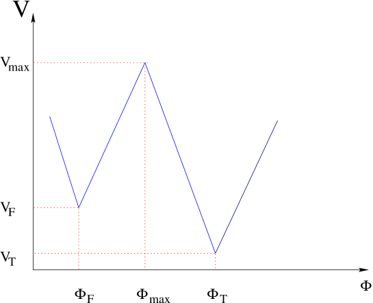
Figure 2: Triangular potential barrier

Appendix B Coleman-Weinberg formula in various dimensions

The CW formula for the one-loop superpotential

$$V_{eff}^{(1)}=\frac{1}{2}\,\text{STr}\int\frac{d^{d}p}{(2\pi)^{d}}\ln(p^{2}+m^{2})$$ (70)

is not always straightforward to compute, since the theory can contain many fields, and one has to diagonalize the squared mass matrices. Some property of the models with metastable vacua can be analyzed without evaluating the eigenvalues of the squared mass matrices of component fields of the theory. To this purpose, we generalize a formula previously given for four-dimensional theories [18] to work in any dimension. Indeed, writing (70) in spherical coordinates and integrating by parts, we have

$$V_{eff}^{(1)} = \frac{\pi^{d/2}}{\Gamma(d/2)}\,\text{STr}\,\int\frac{dp}{(2\pi^{d})}\,p^{d-1}\,\ln(p^{2}+m^{2})$$ (71)

$$= -\frac{1}{d}\,\frac{1}{2^{d-1}\,\pi^{d/2}\Gamma(d/2)}\,\text{STr}\,\int dp\,\frac{p^{d+1}}{p^{2}+m^{2}}$$

where $A_{d}=2\pi^{d/2}/\Gamma(d/2)$ is the d-dimensional spherical surface. By substituting $d=3$ we recover (6).

References

- [1] J. Bagger and N. Lambert, Phys. Rev. D 75, 045020 (2007) [arXiv:hep-th/0611108].
- [2] A. Gustavsson, Nucl. Phys. B 811, 66 (2009) [arXiv:0709.1260 [hep-th]].
- [3] J. Bagger and N. Lambert, Phys. Rev. D 77, 065008 (2008) [arXiv:0711.0955 [hep-th]].
- [4] J. Bagger and N. Lambert, JHEP 0802, 105 (2008) [arXiv:0712.3738 [hep-th]].
- [5] O. Aharony, O. Bergman, D. L. Jafferis and J. Maldacena, JHEP 0810, 091 (2008) [arXiv:0806.1218 [hep-th]].
- [6] D. Martelli and J. Sparks, Phys. Rev. D 78, 126005 (2008) [arXiv:0808.0912 [hep-th]].
- [7] A. Hanany and A. Zaffaroni, JHEP 0810, 111 (2008) [arXiv:0808.1244 [hep-th]].
- [8] A. Hanany, D. Vegh and A. Zaffaroni, JHEP 0903, 012 (2009) [arXiv:0809.1440 [hep-th]].
- [9] S. Franco, A. Hanany, J. Park and D. Rodriguez-Gomez, JHEP 0812, 110 (2008) [arXiv:0809.3237 [hep-th]].
- [10] A. Hanany and Y. H. He, arXiv:0811.4044 [hep-th].
- [11] A. Amariti, D. Forcella, L. Girardello and A. Mariotti, arXiv:0903.3222 [hep-th].
- [12] S. Franco, I. R. Klebanov and D. Rodriguez-Gomez, arXiv:0903.3231 [hep-th].
- [13] J. Davey, A. Hanany, N. Mekareeya and G. Torri, arXiv:0903.3234 [hep-th].
- [14] M. Petrini and A. Zaffaroni, arXiv:0904.4915 [hep-th].
- [15] M. Aganagic, arXiv:0905.3415 [hep-th].
- [16] A. Giveon, D. Kutasov and O. Lunin, arXiv:0904.2175 [hep-th].
- [17] S. Ray, Phys. Lett. B 642 (2006) 137 [arXiv:hep-th/0607172].
- [18] D. Shih, JHEP 0802 (2008) 091 [arXiv:hep-th/0703196].
- [19] Z. Sun, JHEP 0901, 002 (2009) [arXiv:0810.0477 [hep-th]].
- [20] A. Amariti and A. Mariotti, arXiv:0812.3633 [hep-th].
- [21] Z. Komargodski and D. Shih, JHEP 0904, 093 (2009) [arXiv:0902.0030 [hep-th]].
- [22] K. Intriligator, D. Shih and M. Sudano, JHEP 0903 (2009) 106 [arXiv:0809.3981 [hep-th]].
- [23] K. A. Intriligator, N. Seiberg and D. Shih, JHEP 0604, 021 (2006) [arXiv:hep-th/0602239].
- [24] S. Franco and A. M. Uranga, JHEP 0606, 031 (2006) [arXiv:hep-th/0604136].
- [25] H. Ooguri and Y. Ookouchi, Nucl. Phys. B 755, 239 (2006) [arXiv:hep-th/0606061].
- [26] I. Garcia-Etxebarria, F. Saad and A. M. Uranga, JHEP 0705, 047 (2007) [arXiv:0704.0166 [hep-th]].
- [27] A. Giveon and D. Kutasov, Nucl. Phys. B 796, 25 (2008) [arXiv:0710.0894 [hep-th]].
- [28] A. Amariti, L. Girardello and A. Mariotti, JHEP 0612, 058 (2006) [arXiv:hep-th/0608063].
- [29] R. Essig, J. F. Fortin, K. Sinha, G. Torroba and M. J. Strassler, JHEP 0903, 043 (2009) [arXiv:0812.3213 [hep-th]].
- [30] M. J. Duncan and L. G. Jensen, Phys. Lett. B 291 (1992) 109.
- [31] L. M. Carpenter, M. Dine, G. Festuccia and J. D. Mason, Phys. Rev. D 79 (2009) 035002 [arXiv:0805.2944 [hep-ph]].
- [32] E. Witten, arXiv:hep-th/9903005.
- [33] O. Bergman, A. Hanany, A. Karch and B. Kol, JHEP 9910, 036 (1999) [arXiv:hep-th/9908075].
- [34] K. Ohta, JHEP 9910, 006 (1999) [arXiv:hep-th/9908120].
- [35] J. de Boer, K. Hori and Y. Oz, Nucl. Phys. B 500 (1997) 163 [arXiv:hep-th/9703100].
- [36] O. Aharony, A. Hanany, K. A. Intriligator, N. Seiberg and M. J. Strassler, Nucl. Phys. B 499 (1997) 67 [arXiv:hep-th/9703110].
- [37] A. Giveon and D. Kutasov, Nucl. Phys. B 812, 1 (2009) [arXiv:0808.0360 [hep-th]].
- [38] V. Niarchos, JHEP 0811, 001 (2008) [arXiv:0808.2771 [hep-th]].
- [39] A. Armoni, A. Giveon, D. Israel and V. Niarchos, arXiv:0905.3195 [hep-th].
- [40] A. E. Nelson and N. Seiberg, Nucl. Phys. B 416 (1994) 46 [arXiv:hep-ph/9309299].