Self-Regulation of AGN in Galaxy Clusters

Abstract

Cool cores of galaxy clusters are thought to be heated by low-power active galactic nuclei (AGN), whose accretion is regulated by feedback. However, the interaction between the hot gas ejected by the AGN and the ambient intracluster medium is extremely difficult to simulate as it involves a wide range of spatial scales and gas that is Rayleigh-Taylor (RT) unstable. Here we present a series of three-dimensional hydrodynamical simulations of a self-regulating AGN in a galaxy cluster. Our adaptive-mesh simulations include prescriptions for radiative cooling, AGN heating and a subgrid model for RT-driven turbulence, which is crucial to simulate this evolution. AGN heating is taken to be proportional to the rest-mass energy that is accreted onto the central region of the cluster. For a wide range of feedback efficiencies, the cluster regulates itself for at least several $10^{9}$ years. Heating balances cooling through a string of outbursts with typical recurrence times of around 80 Myrs, a timescale that depends only on global cluster properties. Under certain conditions we find central dips in the metallicity of the intracluster medium. Provided the sub-grid model used here captures all its key properties, turbulence plays an essential role in the AGN self-regulation in cluster cores.

1 Introduction

High-resolution observations from the Chandra and XMM-Newton X-ray telescopes have revolutionised our understanding of the hot-intracluster medium (ICM). While a large number of galaxy clusters have strong peaks in their central X-ray surface brightness distributions, indicating that their central gas is cooling rapidly, detailed spectra of such cool-core clusters show that this gas fails to cool below $\approx 1$ keV (e.g.  Peterson et al., 2001; Rafferty et al., 2006; McNamara & Nulsen, 2007). This deficit means that radiative cooling must be balanced by an unknown energy source.

Currently, the most successful model for achieving this balance relies on heating by outflows from an AGN, hosted by the central cD galaxy (e.g.  Churazov et al., 2000; Brüggen & Kaiser, 2002; Magliocchetti & Brüggen, 2007). Galaxies within $0.2r_{200}$ of the centre of groups and clusters show a boosted likelihood of hosting large radio-loud jets of AGN-driven material (Burns, 1990; Best et al., 2005). The energies from such outbursts are comparable to those needed to stop the gas from cooling (e.g.  Simionescu et al., 2008), and the mean power of the outbursts is well-correlated with the radiated power (Bîrzan et al., 2004). Furthermore, AGN feedback from the central cD increases in proportion to the cooling luminosity, as expected in an operational feedback loop (e.g.  Bîrzan et al., 2004; Rafferty et al., 2006).

Yet despite these many clues, the nature of the feedback mechanism is still not understood. In clusters, energy coming from a region less than a parsec across has to regulate a volume of gas that is about a few hundred kpc across. This regulation must maintain the balance between heating and cooling for a long time, at least since a redshift of $z\approx 0.4$ (Bauer et al., 2005). Moreover, it must hold in systems with luminosities that span about three orders of magnitude (Churazov et al., 2005). Finally, the output by the AGN must be regulated by the physical conditions in the vicinity of the AGN, rather than the properties of the host galaxy in which it is contained (Best et al., 2007).

In general, gas can make its way onto an AGN disc directly from the hot gas via Bondi-Hoyle accretion (e.g.  Allen et al., 2006) or in the form of cold blobs (e.g.  Soker, 2006). It is likely that the AGN feedback in clusters is caused by accretion of hot gas onto pre-formed massive black holes in old elliptical galaxies (e.g.  Best et al., 2007; Hardcastle et al., 2007), which produce low-power radio jets but relatively little emission at optical, ultraviolet and infrared wavelengths. On the other hand, the fuelling by cold gas may be responsible for AGN with strong emission lines (e.g.  Hardcastle et al., 2007) but the supply of powerful high-excitation sources does not have a direct connection to the hot phase. Most efforts to explain feedback have concentrated on the hot-accretion scenario.

Churazov et al. (2002) considered a toy model of ICM feedback regulated by hot gas accretion, in which black hole growth was set by the classic Bondi formula, with $\dot{M}\propto n_{e}T^{-3/2}$. For a ratio of specific heats of 5/3, this rate only depends on the entropy and is directly affected by heating and cooling. The ICM in the model responded to the heating by expanding, which lowered the gas density and accretion rate. As the gas radiated away energy, the atmosphere contracted and the accretion rate rose again. Application of the results to the Virgo cluster suggested that accretion proceeded at approximately the Bondi rate down to a few gravitational radii and that most of the power was carried away by an outflow. Comparison of the accretion rate predicted by the Bondi formula with the luminosity of the cooling flow region in M87 suggested a high efficiency for transforming the rest mass of accreted material into mechanical power of an outflow at the level of a few per cent. Recently, Allen et al. (2006) found evidence that the power of outbursts in giant elliptical galaxies scales with the Bondi accretion rate.

However, the full simulation of this feedback cycle remains elusive. Direct simulation of a galaxy cluster from Mpc scales down to the parsec scale at which mass accretes onto the central supermassive black hole is still out of reach even for the latest generation of adaptive-mesh refinement (AMR) codes. Hence, in most hydrodynamical simulations of AGN feedback, the energy input into the ICM is set by hand, rather than computed from the conditions surrounding the central galaxy. Only Vernaleo & Reynolds (2006), Brighenti & Mathews (2006) and Cattaneo & Teyssier (2007) attempted hydrodynamic simulations of self-regulated accretion, and none of these studies was able to reproduce all the observed properties of cool-core clusters.

Vernaleo & Reynolds (2006) carried out a set of three-dimensional cluster simulations in which they took the kinetic energy of the AGN jet to be proportional to the instantaneous mass accretion rate across an inner spherical boundary. They found that their simulations were incapable of balancing heating and cooling as the jet formed a low-density channel, which stopped the hot gas from coupling effectively to the surrounding ICM. A delay between the mass accretion rate and the response of the jet was introduced in further simulations, but could not alleviate this problem. However, Heinz et al. (2006) have shown that in more realistic initial conditions the ambient bulk motions of the ICM prevent the formation of such channels, though their simulations were not self-regulating.

Brighenti & Mathews (2006) simulated self-regulated mass-loaded jets that resemble disk winds. They presented two-dimensional hydrodynamical models where outflows were generated by assigning a fixed velocity to gas that flowed into a biconical source region at the cluster centre. The acceleration of gas in the source cones was triggered when gas flowed into the innermost zones. As the jet proceeded, it entrained additional ambient gas and its mass flux increased. After many gigayears, the time-averaged gas temperature profile resembled observations and very little gas cooled below the virial temperature.

However, feedback is at least partly mediated by low-power Fanaroff-Riley type I (FR I) sources and this has not been simulated before. Cattaneo & Teyssier (2007) carried out three-dimensional simulations in which AGN jets were regulated via a Bondi-accretion rate measured at the cluster centre starting from hydrostatic initial conditions. For their setup, a very violent AGN phase ($L\sim 10^{45}$ erg/s) occurred lasting for about 250 million years, followed by a period of at least 4 gigayears during which the accretion rate of the black hole and the mass of the cold gas in the cluster core stayed constant with a luminosity of a few times $10^{43}$ erg s^-1. This scenario does not explain the recurrent, low-power FR I sources that are observed in local cool-core clusters.

The biggest obstacle to these simulations is that it is still unclear how the mechanical power of the AGN is transformed into thermal energy and distributed throughout the cluster. Nulsen et al. (2007) pointed out that theoretically one would expect the energy to be dissipated locally. As the bubble rises, they argue, the ICM falls inward around it to fill the space it occupied, converting gravitational potential energy to kinetic energy. Details of the flow depend on the viscosity, which is poorly determined. If it is high, the flow is laminar and the kinetic energy is dissipated as heat over a region comparable in size to the cavity. If the viscosity is low, the Reynolds number is high and the flow would form a turbulent region of a similar size to the cavity. Turbulent kinetic energy is dissipated in the turnover time of the largest eddies, so that the dissipation time $t_{\rm diss}\approx r_{b}/v_{\rm turb}$, where $r_{b}$ is the radius of the bubble and $v_{\rm turb}$ is the speed of the eddy, which is comparable to the speed of the cavity. Since $t_{\rm diss}v_{b}\approx r_{b}$, much of the turbulent kinetic energy is dissipated in a region of comparable size to the cavity. Thus, regardless of the viscosity, the kinetic energy created by cavity motion is deposited locally. Other authors have pointed out the importance of sound waves and weak shocks in dissipating heat (Fabian et al., 2003; Brüggen et al., 2007; Sanders & Fabian, 2007, 2008), and considered the possibility that AGN bubbles are stabilized by magnetic fields (De Young 2003; Brüggen & Kaiser 2001; Ruszkowski et al. 2007) or massive jets (Sternberg & Soker, 2008).

In Scannapieco & Brüggen (2008) (SB08 hereafter), we showed that even in the absence of magnetic effects, the evolution of AGN bubbles cannot presently be captured reliably by direct simulations. While pure hydrodynamic simulations indicate that AGN bubbles are disrupted into resolution-dependent pockets of underdense gas, proper modeling of subgrid turbulence indicates that this a poor approximation to a turbulent cascade that continues far beyond current resolution limits. Adding a subgrid model of turbulence and mixing (Dimonte & Tipton, 2006) to the adaptive-mesh hydrodynamic code, FLASH3, we found that Rayleigh-Taylor (RT) instabilities act to effectively mix the heated region with its surroundings, while at the same time preserving it as a coherent structure, consistent with observations. Cattaneo & Teyssier (2007) also pointed out the importance of turbulence in mediating the jet power to the accretion mechanism, although they were unable to resolve it.

In this paper, we explore how a subgrid model for turbulence provides the missing piece necessary to construct a full numerical simulation of a self-regulating jet at the centre of cool-core clusters. Furthermore, with no fine tuning, such simulations naturally explain both the mechanical power of AGN, and their duty cycles. The structure of the paper is as follows: In §2, we describe our method including the algorithm and the setup, and in §3 we present our results. A discussion is given in §4.

2 Method

2.1 Simulation and Turbulence Modeling

Out simulations were performed with FLASH version 3.0 (Fryxell et al., 2000), a multidimensional adaptive mesh refinement hydrodynamics code. It solves the Riemann problem on a Cartesian grid using a directionally-split Piecewise-Parabolic Method (PPM) solver (Colella & Woodward, 1984). While the direct simulation of turbulence is extremely challenging, computationally expensive, and dependent on resolution (e.g.  Glimm et al., 2001), its behaviour can be approximated to a good degree of accuracy by adopting a sub-grid approach. Recently, Dimonte & Tipton (2006), described a sub-grid model that is especially suited to capturing the buoyancy-driven, turbulent evolution of AGN bubbles. The model captures the self-similar growth of the RT and Richtmyer-Meshkov (RM) instabilities by augmenting the mean hydrodynamics equations with evolution equations for the turbulent kinetic energy per unit mass and the scale length of the dominant eddies. The equations are based on buoyancy-drag models for RT and RM flows, but constructed with local parameters so that they can be applied to multi-dimensional flows with multiple materials. The model is self-similar, conserves energy, preserves Galilean invariance, and works in the presence of shocks.

The mean flow fluid equations in this case are given by

$$\frac{\partial{\bar{\rho}}}{\partial t}+\frac{\partial{\bar{\rho}}\tilde{u}_{j}}{\partial x_{j}} = 0,$$ (1)

$$\frac{\partial{\bar{\rho}}\tilde{u}_{i}}{\partial t}+\frac{\partial{\bar{\rho}}\tilde{u}_{i}\tilde{u}_{j}}{\partial x_{j}}+\frac{\partial P}{\partial x_{i}}+\rho\frac{\partial\Phi}{\partial x_{i}} = C_{P}\frac{\bar{\rho}K}{\partial x_{i}},$$ (2)

$$\frac{\partial{\bar{\rho}}E}{\partial t}+\frac{\partial{\bar{\rho}}E\tilde{u}_{j}}{\partial x_{j}}+\frac{\partial P\tilde{u}_{j}}{\partial x_{j}} = \frac{\partial}{\partial x_{j}}\left(\frac{\mu_{t}}{N_{E}}\frac{\partial E}{\partial x_{j}}\right)-S_{K},$$

where $t$ and ${\bf x}$ are time and position variables, $\bar{\rho}({\bf x},t)$ is the average density field, $\tilde{u}_{i}({\bf x},t)$ is the mass-averaged mean-flow velocity field in the $i$ direction, $P({\bf x},t)$ is the mean pressure, $\Phi({\bf x},t)$ is the gravitational potential, and $E({\bf x},t)$ is the mean internal energy per unit mass. The terms on the right hand side of these equations couple the subgrid quantities to the mean flow. These three terms model: (i) the excess “pressure” arising from the turbulent kinetic energy per unit mass $K,$ which is scaled by a constant $C_{P}$; (ii) turbulent mixing, which is modeled as a turbulent viscosity $\mu_{t}$, scaled by a constant $N_{E}$; and (iii) an explicit source term, $S_{K}$ that contains both RT and RM contributions, and removes energy from the mean flow and moves it into the turbulent field. This is given by

$$S_{K}=\bar{\rho}V\left[C_{B}A_{i}g_{i}-C_{D}\frac{V^{2}}{L}\right],$$ (3)

where $V\equiv\sqrt{2K}$ is the average turbulent velocity, $L$ is the turbulent eddy scale, $g_{i}\equiv-(1/\rho)\partial P/\partial x_{i}$ is the gravitational acceleration, the coefficients $C_{B}$ and $C_{D}$ are fit to experiments ($C_{B}=0.84$ and $C_{D}=1.25$) and $A_{i}$ is the Atwood number in the $i$ direction. In the code, we determine this as

$$A_{i}=\frac{\bar{\rho}_{+}-\bar{\rho}_{-}}{\bar{\rho}_{+}+\bar{\rho}_{-}}+C_{A}\frac{L}{\bar{\rho}+L|\partial\bar{\rho}/\partial x_{i}|}\frac{\partial\bar{\rho}}{\partial x_{i}},$$ (4)

where $C_{A}$ is a constant and $\bar{\rho}_{-}$ and $\bar{\rho}_{+}$ are the densities on the back and front boundaries of the cell in the $i$ direction. This source term causes turbulence to decay away at a characteristic time scale of $\approx L/V$ in the absence of external driving, while the growth term causes turbulent velocity to grow at a rate $\dot{V}\approx g,$ whenever the gravitational acceleration opposes the density gradient.

The turbulence quantities that appear in these equations are calculated from evolution equations for $L$ and $K$. The eddy scale $L$ must be evolved because the buoyancy-driven RT and RM instabilities depend on the eddy size, which is expected to grow self-similarly. Simple equations that include diffusion, production, and compression are given by

$$\frac{\partial\bar{\rho}L}{\partial t}+\frac{\partial\bar{\rho}L\tilde{u}_{j}}{\partial x_{j}}=\frac{\partial}{\partial x_{j}}\left(\frac{\mu_{t}}{N_{L}}\frac{\partial L}{\partial x_{j}}\right)+\bar{\rho}V+C_{C}\bar{\rho}L\frac{\partial\tilde{u}_{i}}{\partial x_{i}},$$ (5)

and

$$\frac{\partial\bar{\rho}K}{\partial t}+\frac{\partial\bar{\rho}K\tilde{u}_{j}}{\partial x_{j}}=\frac{\partial}{\partial x_{j}}\left(\frac{\mu_{t}}{N_{K}}\frac{\partial K}{\partial x_{j}}\right)-C_{P}\rho K\frac{\partial\tilde{u}_{i}}{\partial x_{i}}+S_{K},$$ (6)

where $N_{K}$, $N_{L}$, $C_{C},$ and $C_{P}$ are constants ($N_{K}=1.0$, $N_{L}=0.5$, $C_{C}=1/3$ and $C_{P}=2/3$). See Dimonte & Tipton (2006) for details on how these constants are determined. In the $L$ equation the three terms on the right hand side of the equation represent, respectively: turbulent diffusion, growth of eddies through turbulent motions, and growth of eddies due to motions in the mean flow. In the $K$ equation the three terms on the right hand side represent, respectively: turbulent diffusion, the work associated with the turbulent stress, and the source term $S_{K},$ which also appears in the internal energy equation to conserve energy. Finally, the turbulent viscosity is calculated as

$$\mu_{t}=C_{\mu}\bar{\rho}L\sqrt{2K},$$ (7)

where $C_{\mu}$ is a constant. Further details of this model and our implementation are given in SB08.

All our simulations are performed in a cubic three-dimensional region with reflecting boundaries that is 680 kpc on a side, although the cool-core region in which we are most interested lies within $\lesssim 100$ kpc of the center. For our grid, we chose a block size of $8^{3}$ zones and an unrefined root grid with $8^{3}$ blocks, for a native resolution of 10.6 kpc. The refinement criteria are the standard density and pressure criteria, and we allow for 4 levels of refinement beyond the base grid, corresponding to a minimum cell size of 0.66 kpc, and an effective grid of 1024³ zones. In all zones $K$ is initialized to $10^{-10}(p/\rho)/2.$ and $L$ is initialized to $10^{-5}\sqrt{p/\rho}\sqrt{1/G\rho}.$

2.2 Cluster Profile

For our overall cluster profile, we adopted the model described in Roediger et al. (2007), which was constructed to reproduce the properties of the brightest X-ray cluster A426 (Perseus) that has been studied extensively with Chandra and XMM-Newton. In this case, the electron density $n_{\rm e}$ and temperature $T_{\rm e}$ profiles are based on the deprojected XMM-Newton data (Churazov et al., 2003) which are in broad agreement with the Chandra data (Schmidt et al., 2002; Sanders et al., 2004); namely:

$$n_{\rm e}=\frac{4.6\times 10^{-2}}{[1+(\frac{r}{57})^{2}]^{1.8}}+\frac{4.8\times 10^{-3}}{[1+(\frac{r}{200})^{2}]^{0.87}}~{}~{}~{}{\rm cm}^{-3},$$ (8)

and

$$T_{\rm e}=7\times\frac{[1+(\frac{r}{71})^{3}]}{[2.3+(\frac{r}{71})^{3}]}~{}~{}~{}{\rm keV},$$ (9)

where $r$ is measured in kpc. Furthermore, the hydrogen number density was assumed to be related to the electron number density as $n_{H}=n_{\rm e}/1.2$. The static, spherically-symmetric gravitational potential, $\Phi(R),$ was set such that the cluster was in hydrostatic equilibrium.

As in Scannapieco & Brüggen (2008), we computed the radiative losses in each cell in the optically-thin limit, with an emissivity $\epsilon=\Lambda(T)n_{H}n_{e}$ where $n_{H}$ and $n_{e}$ are the number density of hydrogen and electrons, respectively, and the cooling function $\Lambda(T)$ describes radiative losses from the optically thin plasma, as in Sarazin (1986) (see also Raymond et al., 1976; Peres et al., 1982).

The metal injection rate in the central galaxy was assumed to be proportional to the light distribution, and modeled with a Hernquist profile given by

$$\dot{\rho}_{\mathrm{metal}}(r,t)=\frac{\dot{M}_{\mathrm{metal}}{}_{0}}{2\pi}\,\frac{a}{r}\,\frac{1}{(r+a)^{3}},$$ (10)

with a scale radius of $a=10$ kpc and a total metal injection rate of $\dot{M}_{\mathrm{metal}}{}_{0}=9.5\times 10^{4}\,M_{\odot}\,\textrm{Myr}^{-1}.$ This is the integral mass injection rate for all elements heavier than helium. The sources of metals are supernovae Ia and stellar mass loss (Rebusco et al., 2005).

In order to be able to trace the metal distribution, we utilize a mass scalar to represent the local metal fraction in each cell, $F\equiv\rho_{\mathrm{metal}}/\bar{\rho}.$ Hence, the quantity $F\bar{\rho}$ gives the local metal density, $\rho_{\mathrm{metal}}$, which has a continuity equation including the metal source, given by

$$\frac{\partial{\bar{\rho}}F}{\partial t}+\frac{\partial{\bar{\rho}}F\tilde{u}_{j}}{\partial x_{j}}=\frac{\partial}{\partial x_{j}}\left(\frac{\mu_{t}}{N_{F}}\frac{\partial F}{\partial x_{j}}\right)+\frac{\dot{\rho}_{\mathrm{metal}}}{\bar{\rho}}$$ (11)

where $N_{F}$ is a dimensionless constant. Furthermore, we assumed that the metal fraction is small at all times. Hence, we could neglect $\dot{\rho}_{\mathrm{metal}}$ as a source term in the continuity equation for the gas density. Also, the mass fraction can be scaled to any value in post-processing.

2.3 AGN Feedback

Bubbles in the ICM are thought to be inflated by a pair of ambipolar jets from the central AGN that inject energy into small regions at their terminal points, which expand until they reach pressure equilibrium with the surrounding medium (Blandford & Rees, 1974). The result is a pair of underdense, hot bubbles on opposite sides of the cluster centre. In order to produce such bubbles, we injected energy into two small spheres of radius $r_{\rm bubble},$ each a distance $r_{\rm bubble}$ from the centre.

Unlike in our previous simulations, the energy input rate was not predetermined, but instead calculated from the instantaneous conditions near the centre of the cluster. In particular, we considered a model in which a fixed fraction of the gas within the central 3 kpc of the cluster accretes onto the central supermassive black hole within a cooling time, and a fixed fraction of the $mc^{2}$ rest mass energy of this accreted gas is returned to the ICM by increasing the pressure within the bubble regions. This is similar to the approach taken by Vernaleo & Reynolds (2006), who calculated AGN feedback based on the mass inflow rate along the 10 kpc inner boundary of a spherical grid. Here our choice of the volume within $3$ kpc of the cluster centre is taken to sample the conditions as near to the central supermassive black hole as possible, while still averaging over enough cells to avoid numerical effects.

The efficiency of gas accretion in powering the bubbles was chosen by scaling to typical numbers observed in galaxy clusters. We took the rate of change of the pressure within the bubble regions to be given by

$$\frac{3}{2}\dot{P}_{\mathrm{inj}}(t)\frac{4\pi}{3}r_{\rm bubble}^{3}=E_{\rm bubble}\frac{75{\rm Myrs}}{t_{\rm cool,3kpc}(t)}\frac{M_{\rm gas,3kpc}(t)}{M_{\rm gas,3kpc}(0)},$$ (12)

where $t_{\rm cool,3kpc}(t)$ is calculated by dividing the total internal energy of the gas within the central 3 kpc by the total radiation rate in this regions, and $M_{\rm gas,3kpc}(t)$ is the total gas within the central 3 kpc, and $E_{\rm bubble}\approx 5\times 10^{59}$ ergs corresponds to the typical energies necessary to inflate the X-ray cavities observed in cool-core clusters (e.g.  Forman et al., 2007), which are generated approximately every 75 Myrs. This prescription corresponds to an overall efficiency of $3.2\times 10^{-3}E_{\rm bubble}/10^{60}{\rm ergs}$ of the $mc^{2}$ energy of the mass cooling rate within the central 3 kpc. Note that choosing a typical value of $E_{\rm bubble}\approx 5\times 10^{59}$ ergs would mean that our energy input is only about $4\times 10^{-5}$ of the rest mass energy of the mass cooling rate within the central $10$ kpc, and thus our models generally have energy input levels similar to that considered by Vernaleo and Reynolds (2006).

Finally, we started all runs with an initial pair of bubbles overpressured by a factor of

$$P_{\rm bubble}(0)\frac{4\pi}{3}r_{\rm bubble}^{3}=E_{\rm bubble},$$ (13)

so as to create some initial “seed” turbulence, to help increasing mixing at early times and speed the simulations towards their eventual quasi-steady states. The choices of $E_{\rm bubble}$ and $r_{\rm bubble}$ for each of the runs carried out in this study are given in Table 1.

Table 1: Run Parameters

Run	Subgrid	$E_{\rm bubble}$	$r_{\rm bubble}$
Name	Model	(ergs)	(kpc)
N5-10	No	$5\times 10^{59}$	10
D5-10	Yes	$5\times 10^{59}$	10
D5-8	Yes	$5\times 10^{59}$	8
D5-12	Yes	$5\times 10^{59}$	12
D2-10	Yes	$2\times 10^{59}$	10
D10-10	Yes	$1\times 10^{60}$	10
D20-10	Yes	$2\times 10^{60}$	10

3 Results

3.1 Self-regulating Oscillations

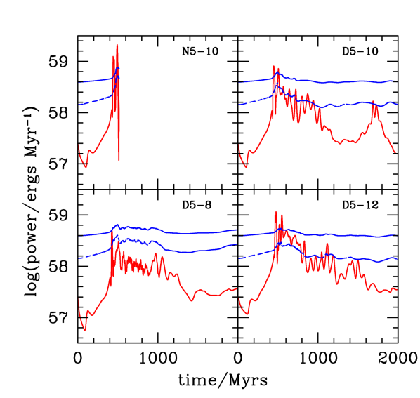
Figure 1: Bubble power and integrated cooling rates for D5-10 (top left), N5-10 (top right), D5-8 (bottom left) and D5-12 (bottom right). The solid blue lines shows the cooling losses in the entire simulation volume, the dashed blue line show the cooling losses in the central 100 kpc of the cluster and the red line shows the energy put into bubbles. The lines for our fiducial run without a subgrid turbulence model (named N5-10) stop at about 450 million year because this is where catastrophic cooling in the centre halted the simulation.

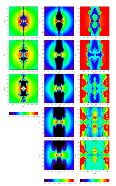
Figure 2: Slices of $\log(\rho/{\rm g\,cm^{-3}})$ (1st column for N5-10 and 2nd column for D5-10) and $\log$ turbulent diffusion time in Myrs (3rd column for D5-10) for times near to when the non-turbulent run cools catastrophically. From top to bottom $t=$ 460, 480, 500, 520 and 540 Myrs.

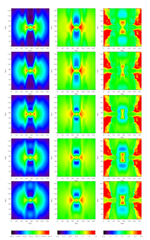
Figure 3: Slices of $\log(\rho/{\rm g\,cm^{-3}})$ (1st column), $\log$ sound crossing time in Myrs (2nd column), and $\log$ turbulent diffusion time in Myrs (3rd column), as the fiducial subgrid run (D5-10) executes a full $\approx 80$ Myr cycle as described in the text. From top to bottom $t=$ 600, 620, 640, 660 and 680 Myrs (all from D5-10).

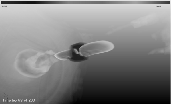
Figure 4: Volume rendering of the temperature in our fiducial run D5-10 at t= 630 Myrs. The blue ring shows the cool gas accreting onto the centre; the red and yellow blobs represent the hot gas ejected by the AGN. On the left side one can see an older bubble from an earlier outburst.

As a control case, we first present the results of a model without subgrid turbulence (5N-10) in which we have chosen $E_{\rm bubble}\approx 5\times 10^{59}$ ergs and $r_{\rm bubble}=10$ kpc. The evolution of the cooling and AGN heating in this case is summarised in the top left panel in Fig. 1. Here we see that the bubbles do not couple to the central region that determines the activity of the AGN. Instead, cool gas accumulates in the centre, increasing the AGN output as shown in this figure, as well as leading to the cold dense central regions shown in Fig. 2. This cooling eventually leads to a drastic outburst of the AGN, which is apparent in a sharp upturn in the heating rate in Fig. 1, and the large empty cavities in the third row in Fig. 2. However this heating does not stop the flow of gas onto the AGN along the midplane. Instead cooling increases catastrophically and we are forced to stop the simulation.

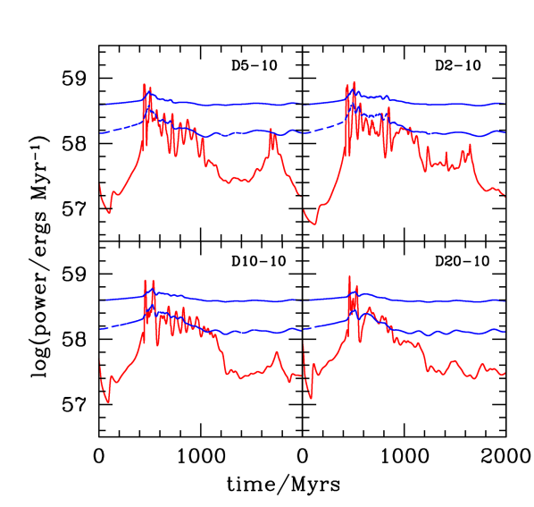
Figure 5: Bubble power and integrated cooling rates for D5-10 (top left), D2-10 (top right), D10-10 (bottom left) and D20-10 (bottom right). Meaning of lines as in Fig. 1.

On the other hand, when the subgrid model for the turbulence is switched on, as in run 5D-10, the bubbles couple much more effectively to the central region. As seen in the second and third columns of Fig. 2, the cold gas that forms in a ring around the ICM, shown in white, is slowly eroded and the AGN activity subsides. The turbulent diffusion or turn-over time, $L/V,$ is plotted in the third column of Fig. 2. It shows that near the ring of cool gas in the centre of the cluster this time is of the order of 80 Myrs. This turbulence mixes in hot material near the centre of the cluster, heating the cool inflowing ring of intracluster gas and stopping the AGN outburst.

Thus instead of cooling catastrophically, the cluster in the simulation with subgrid turbulence begins to execute a series of oscillations as indicated in Fig. 3. The top row of this plot shows the configuration at 600 Myrs, shortly after an outburst of AGN activity. From this time to 640 Myrs, turbulence decays away at the turn-over time scale, $L/V,$ and mixing near the cluster center becomes progressively less efficient. This leads to an increased level of accretion near the core, as more and more cold gas makes its way onto the AGN. The result is a new burst of AGN activity, which drives a bubble on the order of a sound crossing time. The RT-unstable bubble leads to a rise of the turbulent viscosity and mixing, which quickly quenches accretion when the turbulent length scale grows to be of the order of the scale of the accretion flow. At this point the AGN remains relatively quiescent until the turbulence decays again on a time of order $L/V$, repeating the cycle as shown in the bottom panels of Fig. 3. This interaction of the AGN-heated regions with the cool inflowing gas is also illustrated in the volume-rendered image shown in Fig. 4.

It is important to point out that we did not tweak the parameters of the subgrid model to achieve the self-regulating cycle. Instead, these parameters are determined by experimental studies of the RT instability and are the same as those employed in Scannapieco & Brüggen (2008). Note also that the time scale for this cycle is not the sound crossing time $l/c_{s}$ for the central region, which is of the order of 10 Myrs. Instead the period between the episodes of AGN fueling is determined by the time it takes for the turbulence to decay away after it has begun to mix the cold gas in the cluster centre. This is given by

$$t_{\rm duty}\approx l/v_{\mathrm{turb}},$$ (14)

where $l$ is the distance between the accretion region of the AGN and the heating region. In our fiducial simulation, $l=r_{\rm bubble}=10$ kpc and is clearly resolved. $v_{\mathrm{turb}}$ is a typical turbulent velocity, which we assume grows in a dynamical time given by $v_{\mathrm{turb}}\sim gt\sim gl/c_{s}$, and $c_{s}$ is the sound speed. Because the cluster is in hydrostatic balance, the gravitational acceleration, $g$ can be written as

$$g=c_{s}^{2}\frac{1}{\rho}\frac{d\rho}{dr}\equiv c_{s}^{2}/r_{0}.$$ (15)

This leads to the turbulent velocity

$$v_{\mathrm{turb}}=gl/c_{s}\approx c_{s}\frac{l}{r_{0}},$$ (16)

and

$$t_{\rm duty}\approx\frac{r_{0}}{c_{s}}.$$ (17)

According to this estimate the turbulent speed is given by $c_{s}l/r_{0}$, which is roughly 700 km s^-1 (10 kpc/ 60 kpc) $\sim 100$ km s ^-1, which is indeed what we find in our simulations. This means that the size of the bubbles does not enter the expression for the duty cycle as would be expected in a cycle regulated by laminar flow. It is the properties of the cluster itself, rather than the jet physics of the central radio source that are setting the recurrence time of the bubbles. Thus the size of the bubbles themselves should not affect the recurrence time of the AGN that we see in Fig. 1 - 3. For the cluster simulated here, the central sound speed is around 700 km s^-1, the scale height of the cluster, $r_{0}$, is around 60 kpc so the duty cycle is 60 kpc / 700 km s${}^{-1}\approx 80$ Myrs.

To test this hypothesis we have varied the geometry of the injection region, leading to the heating and cooling evolution shown in the lower panels of Fig. 1. As in run D5-10, the time between two subsequent outbursts for runs D5-8 and D5-12 is roughly 80 Myrs. Also, in all cases the activity goes down when the cool core has been destroyed by recurrent AGN activity. Again, this large overall time scale, which is $\approx 1$ Gyr, is not dependent on the particulars of bubble injection. Rather it is the time it takes for the turbulence to dissipate through the cool core of the clusters, which is given by

$$t_{\rm cc}\approx R_{\rm cc}/v_{\mathrm{turb}}\approx 100\,{\rm kpc}/100\,{\rm km/s}\approx 1\,{\rm Gyr}\ .$$ (18)

After this the core has been heated sufficiently to stop the gas inflow. It then takes a central cooling time of about 1 Gyr for the cool core to reform and the intermittent AGN activity to resume.

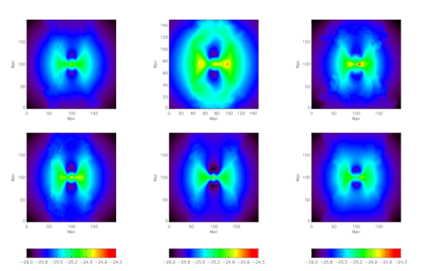
Figure 6: Slices of the logarithm of the density at 1 Gyr. Top from left to right: D5-10, D5-8, D5-12 Bottom from left to right: D2-10, D10-10, D20-10.

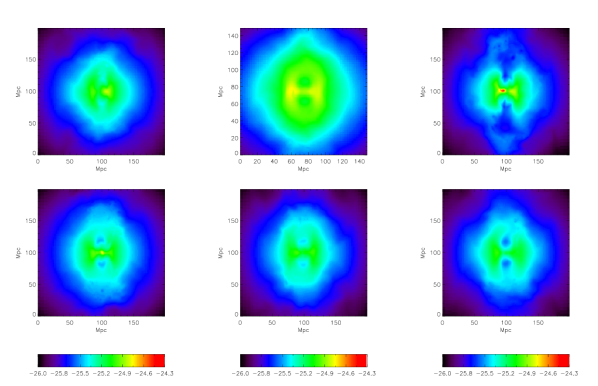
Figure 7: Slices of the logarithm of the density at 1.5 Gyr. Top from left to right: D5-10, D5-8, D5-12. Bottom from left to right: D2-10, D10-10, D20-10.

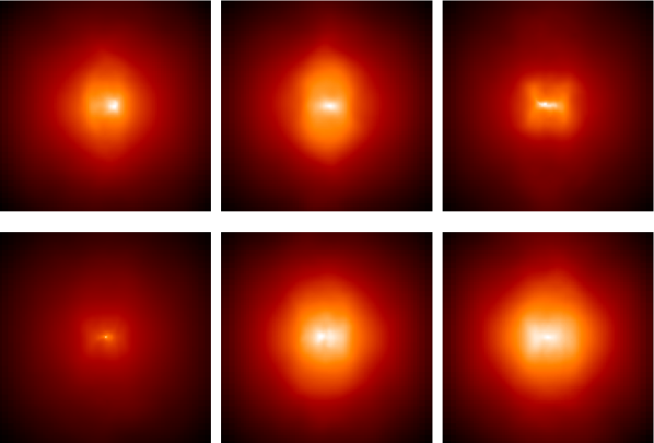
Figure 8: X-ray maps (projections of $\Lambda(T)n_{H}n_{e}$) at 1 Gyr, projected perpendicular to the bubble axis. Top from left to right: D5-10, D5-8, D5-12. Bottom from left to right: D2-10, D10-10, D20-10.

Figure 9: X-ray maps (projections of $\Lambda(T)n_{H}n_{e}$) at 1.5 Gyr, projected perpendicular to the bubble axis. Top from left to right: D5-10, D5-8, D5-12. Bottom from left to right: D2-10, D10-10, D20-10.

In Fig. 5, we vary the efficiency with which inflowing rest mass energy is converted into thermal energy deposited by the AGN. The heating/cooling curves for runs D2-10, D5-10 and D10-10 look remarkably similar. Even with different efficiencies, the AGN easily regulates itself and the resulting duty cycles are largely unchanged.

In fact, the only run that shows a noticeably different evolution history is the high energy D20-10 case. Although this case shows a strong AGN event after about 400 Mrs as in the other runs, unlike the other runs the energy injection remains relatively weak at late times and varies irregularly. So, provided the energy is injected sufficiently far from the region that determines the fuelling of the AGN and provided the heating rate is not so high as to destroy the cool core immediately, the duty cycle is independent of the exact choice of parameters.

3.2 Overall Cluster Properties

Slices of the density through the cluster centre at $t=1$ Gyr and $t=1.5$ Gyr are shown in Fig. 6 - 7, all plotted on the same colour scale. In these figures, the top rows show results from runs with varying bubble sizes at a fixed feedback efficiency, and the bottom rows show results from runs with varying efficiencies at a fixed bubble size. The $t=1$ Gyr slices shown in Fig. 6 correspond to a time shortly after a major outburst has taken place in each of the runs. One can see large plumes streaming from the centre in all cases, although these are somewhat weaker in the D5-8 run than in the other runs. In general, the size of the energy injection region has a stronger impact on the appearance of the cluster than the choice of feedback efficiency, as one would expect for a self-regulating cycle, in which feedback increases only to the level necessary to balance cooling. In fact, for efficiencies that vary by a factor of 10, the density distributions look remarkably similar. In the $t=1.5$ Gyr slices, shown in Fig. 7, one only sees traces of the AGN activity in the form of bubbles of radius $\approx 10$ kpc on either side of the centre. Again these bubbles are clearly seen in all runs, and the variance between runs is more strongly dependent on geometry than feedback efficiency.

X-ray maps corresponding to the same times as in the density slices are shown in Figs. 8 and 9. For simplicity we construct these by projecting the full cooling emissivity as computed from $\epsilon=n_{H}n_{e}\Lambda(T)$ as described in §2.2. Because the emissivity is proportional to the square of the density, the X-ray images are dominated by the emission from the cluster centre, and demonstrate the same overall peaked distribution observed in nearby cool-core clusters (e.g.  Sarazin, 1986). On closer inspection, one can also see substructure and signatures of the AGN-blown cavities. In the 1 Gyr profiles, for example, many runs show clear evidence of circular cavities that are surrounded by brighter emission, especially on the sides. This is particularly clear in run D5-12, which at 1 Gyr contains a large X-shaped structure that resembles the X-ray image of the Virgo elliptical M84 (Finoguenov et al., 2008). In all the runs, and unlike in all previous attempts to simulate self-regulating AGN, the appearance of our self-regulated AGN in X-rays resembles observations of nearby clusters (e.g.  Fabian et al., 2003; McNamara et al., 2005; Nulsen et al., 2005; Forman et al., 2007; Kraft et al., 2007).

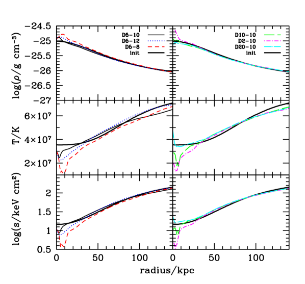
Figure 10: Profiles of density (top), entropy (middle) and emission-weighted temperature (bottom) at 1.0 Gyr. In all panels the fat solid line shows the initial profile. Left panels: solid: D5-10; dotted: D5-12 and short dashed: D5-8. Right panels: long dashed: D10-10; dot-short dashed: D2-10 and dot-long dashed: D20-10.

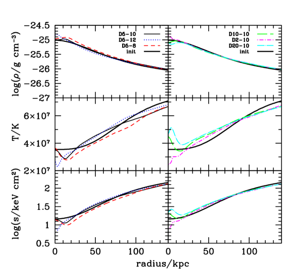
Figure 11: Profiles of density (top), entropy (middle) and emission-weighted temperature (bottom) at 1.5 Gyr. In all panels the fat solid line shows the initial profile. Left panels: solid: D5-10; dotted: D5-12 and short dashed: D5-8. Right panels: long dashed: D10-10; dot-short dashed: D2-10 and dot-long dashed: D20-10.

The radial profiles of average density, emission-weighted temperature, and entropy are shown in Figs. 10 - 11. Here the density is given by an average over the solid angle, $\Omega$, as

$$\bar{\rho}(r)=\frac{1}{4\pi}\int d\Omega\,\bar{\rho}(r,\Omega),$$ (19)

the emission-weighted temperature is given by

$$T_{\rm EW}(r)=\frac{\int d\Omega\,\epsilon(r,\Omega)\,T(r,\Omega)}{\int d\Omega\,\epsilon(r,\Omega)},$$ (20)

and the radial entropy profiles is calculated from the emission-weighted temperature according to

$$S(r)=k_{\rm B}T_{\rm EW}(r)n_{\rm e}(r)^{-2/3}.$$ (21)

In these figures, the right columns show the runs with varying efficiencies, D2-10, D5-10 and D10-10, and the left columns show the runs with different injection geometries, D5-8, D5-10 and D5-12.

Across the runs and at both time steps, the density contours deviate very little from the initial profile, as shown by the thick solid lines. On the other hand, there are noticeable changes in the temperature, which are also reflected in the entropy profiles. These differences are largest within 50 kpc, and at these distances, the profiles at 1 Gyr show that significant cooling is going on at the cluster centre. The clusters are caught in the midst of ongoing feedback oscillations, and because these oscillations are not in phase with each other, $T_{\rm EW}(R)$ and $S(R)$ at these small radii vary significantly across runs.

Outside of 50 kpc, more subtle changes in temperature and entropy can be seen. In the left panels, in which the geometry of the bubbles is varied, the D5-8 run leads to slightly lower temperature and entropy profiles, the fiducial D5-10 stays close to the original profile, and the D5-12 run leads to a slight increase in temperature and entropy. The cluster as a whole is finding a slightly different equilibrium, which is weakly dependent on the geometry of energy input. On the other hand, in the right panels, in which the feedback efficiency is varied, all runs maintain $T_{\rm EW}(R)$ and $S(R)$ profiles which are indistinguishable from each other. Again this similarity is indicative of self-regulation and occurs in spite of an order of magnitude variation in feedback efficiency.

By $t$ = 1.5 Gyr, the central oscillations have died down and the central entropies have been raised to values $\geq 10$ keV cm². Outside of this core region, the profiles have evolved slightly in the D5-8 and D5-12 cases, and are very similar to the initial state for all runs with $r_{\rm bubble}=10$ kpc. As is observed in cool-core clusters, the AGN has managed to maintain the original entropy propfile in the face of widespread cooling. As we start already with a cluster profile that has non-zero core entropy, we cannot say much about the origin of the entropy floor in non-cool-core clusters (Cavagnolo et al., 2009). However, these simulations, that cover a long physical time and many AGN outbursts, suggest that it is difficult to boost the core entropy to values $\approx 100$ keV cm² with a string of relatively weak outbursts.

Finally, in Fig. 12 we plot the metallicity in our simulated clusters. While previous simulations have modeled the effect of AGN activity on metals profiles (e.g.  Tornatore et al., 2004; Brüggen, 2002), none of these have been self-regulating. As a result of the intermittent AGN activity, the metals are distributed over a large volume. Both metal density and metallicity are plotted in Fig. 12, which shows that the AGN is effective at transporting metals.

A secondary maximum develops in the metallicity, which moves outward at around 20 km/s. As a result, the profiles of the metallicity at times 1200, 1600 and 2000 Myr show dips near the centre. This might explain the abundance dips in the iron distribution that have been observed in the Perseus and Centaurus clusters (e.g.  Matsushita et al., 2007; Sanders et al., 2004, and for a discussion on metal abundance patterns in clusters also see Simionescu et al. 2008). In Perseus, the iron abundance dips from above 0.6 solar at around 40 kpc to below 0.5 solar near 15 kpc from the centre, and these numbers are similar to what we find here. However, unlike Perseus, the metal abundance in our simulations increases again in the very centre of the cluster, although this would not occur if the metal production had slowed down over time (Renzini et al., 1993). Future simulations with a time-dependent metal production rate might shed further light on the origin of metallicity dips in some galaxy clusters.

The profiles of the turbulent parameters, $L$ and $K$, which we have not plotted here, look very similar across runs. Over most of the cluster, the turbulent velocities are $\leq 100$ km s${}^{-1},$ and the turbulent kinetic energy peaks at a radius $\approx 20$ kpc, at the outer edge of the bubbles where the turbulence is driven. The magnitude of turbulent velocities is in line with studies of resonant scattering in the ICM that find that the isotropic turbulent velocities on spatial scales smaller than 1 kpc are less than 100 km/s (Werner et al. 2009).

The effective turbulent diffusivities produced by the intermittent AGN are of the order of 500 kpc km/s (Rebusco et al., 2005). David & Nulsen (2008) have probed the Fe distribution in eight cool-core clusters and find that the Fe is significantly more extended than the stellar mass in the central galaxy. They find that diffusion coefficients of 300-3000 kpc km/s are required to produce the observed Fe profiles. Based on these inferred diffusion coefficients, they conclude that heating by turbulent diffusion of entropy and turbulent dissipation can balance the radiative losses in their sample. Our simulations confirm this. In real clusters, other factors such as mergers may contribute to the broadening of the metallicity distribution. However, the magnitude of metal transport in galaxy clusters can be explained by the action of AGN alone.

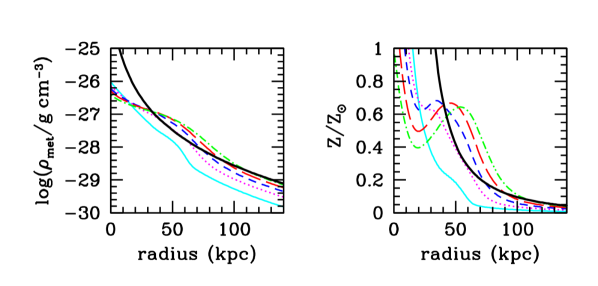
Figure 12: Left: metal density of our fiducial run D5-10 at times t=400, 800, 1200, 1600 and 2000 Myr. The sold black line shows the expected metal density after 2 Gyr in the absence of any AGN activity. Right: The corresponding metallicity in units of solar metallicity (50 times metal mass fraction). Note that times 1200, 1600 and 2000 Myr show metallicity dips near the centre.

4 Discussion

In this study, we have developed a complete and self-consistent three-dimensional model of AGN self-regulation in cool core clusters. In this picture cooling is balanced by periodic energy input from buoyant radio bubbles, whose turbulent evolution couples them to the inflowing cool gas, through mixing on scales that presently can only be captured with subgrid modeling. When turbulence is property accounted for, our model manages to regulate itself for a range of geometries and feedback efficiencies. A phase of episodic heating is followed by a phase in which the AGN is quiet as the cool core reforms, which is followed in turn by another phase of episodic heating. Turbulence also helps to isotropise the injected energy over a turbulent timescale and remedies the problem of channel formation reported by Vernaleo & Reynolds (2006). Our results reproduce a number of key features seen in X-ray observations including:

• temperature, density and entropy profiles that stay fairly monotonous over time, despite rapid cooling near the cluster centre;

• X-rays profiles that are strongly peaked towards the core, and show clear evidence of large bubble cavities rising towards the cluster outskirts; and

• metals that are well mixed into the outer regions of the cluster and exhibiting metallicity “dips” near the cluster centre.

Despite these successes, however, there are a number of areas in which our model remains incomplete. In our approach, feedback is controlled by the total mass inflow through a sphere of $r=3$ kpc, ignoring the details of the inner accretion flow, which will go through various phases as revealed by optical observations of filaments (e.g.  Fabian et al., 2008). Furthermore, our simulations do not include radiative heating, star formation, thermal conduction, cosmic rays, or magnetic fields. However, it is unclear how important these processes are for AGN self-regulation. While thermal conduction may be important in establishing the self-similar entropy profiles found outside cluster cores (Cavagnolo et al., 2009), its role in the cool cores of clusters is uncertain. Similarly, while cosmic rays are unlikely to supply much pressure support in galaxy clusters, cosmic-ray pressure gradients lead to convection, which in turn heats the ICM by advecting internal energy inward and allowing the cosmic rays to do $p\,dV$ work on the thermal plasma (Chandran & Rasera, 2007). Recently, there has also been renewed interest in the effect of magnetic fields on the dynamics of the ICM, which is subject to a number of instabilities including the magnetothermal instability (Balbus, 2000; Parrish & Quataert, 2008) and the heat-flux driven buoyancy instability (Parrish et al., 2008). These instabilities can lead to large-scale convective motions under a wide range of conditions. However, as demonstrated by numerical simulations (Parrish et al., 2008), these motions tend to shut themselves off and thus do not play a major role in cool-core heating. Nonetheless, in future simulations, each of these effects should be explored.

The evolution of AGN in clusters involves an enormous range of time-scales, from the few days characteristic of the dynamical time at the event horizon to the few gigayears required for the development of a cooling catastrophe in the cluster core. Here we advance a new explanation for the physics that determines the frequency of the intermittent bubbles that regulate cool-core clusters. Turbulence is crucial for mediating the heat input by AGN to the region that fuels the supermassive black hole, and thus the time scale for the process is determined by the turbulent turn-over time. This time scale, which is around a few $10^{7}$ years in our simulations, is given by the cluster scale radius divided by the central sound speed, and thus depends on overall cluster properties rather than the details of energy injection.

A number of observational methods have been employed to quantify how long an average radio source spends in an active state and the time between active phases. One method invokes spectral ageing and lobe expansion speed arguments (Alexander & Leahy, 1987), yielding times of a few $10^{7}$ years. Energy injection rates required to quench cooling flows point to time-scales of the order of few $10^{7}$ to $10^{8}$ years (e.g.  Owen & Eilek, 1998; McNamara et al., 2005; Nulsen et al., 2005). Observations of multiple cavities in the Perseus and Virgo clusters also suggest times $\approx 10^{8}$ years between subsequent outbursts of the radio-loud AGN. Low-frequency radio surveys in clusters might also reveal radio ghosts whose synchrotron ages will provide important clues about the histories of self-regulating radio-loud AGN.

References

- Alexander & Leahy (1987) Alexander P., Leahy J. P., 1987, MNRAS, 225, 1
- Allen et al. (2006) Allen S. W., Dunn R. J. H., Fabian A. C., Taylor G. B., Reynolds C. S., 2006, ArXiv Astrophysics e-prints
- Bîrzan et al. (2004) Bîrzan L., Rafferty D. A., McNamara B. R., Wise M. W., Nulsen P. E. J., 2004, ApJ, 607, 800
- Balbus (2000) Balbus S. A., 2000, ApJ, 534, 420
- Bauer et al. (2005) Bauer F. E., Fabian A. C., Sanders J. S., Allen S. W., Johnstone R. M., 2005, MNRAS, 359, 1481
- Best et al. (2005) Best P. N., Kauffmann G., Heckman T. M., Brinchmann J., Charlot S., Ivezić Ž., White S. D. M., 2005, MNRAS, 362, 25
- Best et al. (2007) Best P. N., von der Linden A., Kauffmann G., Heckman T. M., Kaiser C. R., 2007, MNRAS, 379, 894
- Blandford & Rees (1974) Blandford R. D., Rees M. J., 1974, MNRAS, 169, 395