Models of granular ratchets

Abstract

We study a general model of granular Brownian ratchet consisting of an asymmetric object moving on a line and surrounded by a two-dimensional granular gas, which in turn is coupled to an external random driving force. We discuss the two resulting Boltzmann equations describing the gas and the object in the dilute limit and obtain a closed system for the first few moments of the system velocity distributions. Predictions for the net ratchet drift, the variance of its velocity fluctuations and the transition rates in the Markovian limit, are compared to numerical simulations and a fair agreement is observed.

1 Introduction

A Brownian ratchet is a system designed to extract work, usually in the form of a net drift or current, from a thermal bath. If the bath is at equilibrium, i.e. it is characterized by only one temperature, a ratcheting behavior is prevented by the second principle of thermodynamics. The system must be coupled to different baths at different temperatures, or to additional specific non-conservative (e.g. time-dependent) forces, in order to escape the consequences of the second principle. Moreover, to observe a net drift, spatial symmetry must also be broken [1, 2, 3]. Dissipation of energy in inelastic collisions between macroscopic grains [4], breaks the time-reversal symmetry and leads to the introduction of suggestively simple models of inelastic Brownian ratchets, which are apparently coupled to only one thermal bath at a single temperature. It is known, for instance, that a granular object, surrounded by a stationary inelastic gas and characterized by a left-right asymmetry, presents a rectification of thermal fluctuations [5] [6] resulting in a net drift in a given direction: the asymmetry of the object can originate from its shape or its inelasticity profile (i.e. different inelasticities on different portions of the surface). Interestingly, the probability density function (pdf) $P(V)$ of the object velocity results asymmetric when its mass $M$ is of the same order or smaller than that of surrounding disks [7]: such an effect is stronger the smaller the elasticity. In this study we intend to offer an analysis of a general model which includes all ingredients cited above, treating also the dynamics of the surrounding gas. This will make clear the conditions required to decouple the gas dynamics from that of the object, making the latter obey a closed Markovian master equation. In this limit we will obtain some general formula for the net drift of the object, its velocity variance and the transition rates of the Markov process, which in general do not satisfy detailed balance. These results compare very well with numerical simulations. The present article is organized as follows: in Sec.2 we introduce the model and obtain the coupled equations of evolution for the probability distributions of the velocities of the ratchet and of the gas, in Sec.3 instead of solving directly the former equations we consider the governing equations for the moments of the distributions, while in Sec. 4 we specialize our study to the case of an equilateral triangle, while in Sec 5 we conclude with a brief summary. Finally, we provide an appendix containing the necessary formulas for the coefficients entering the equations of Sec.3

2 Theory

Our 2D model consists of a rigid convex object of mass $M$, generally asymmetric, surrounded by a dilute gas of $N$ hard disks of mass $m$ and density $n=N/A$ where $A$ is the area of the box. The surface of the object, of perimeter $C$, has a non-homogeneous inelasticity with a coefficient of restitution that depends on the point of contact on the surface. The object can only slide, without rotating, along the direction $x$. The collisions between two disks of the gas are dissipative with a coefficient of restitution $\alpha_{dd}$. In this system the energy is not conserved and an external driving mechanism is needed to attain a stationary state. In order to maintain this steady state the gas is coupled to a thermal bath [8]: the gas particles between two collisions are subject to an external random force. The dynamics of the object is assumed not to couple directly with the thermostat, but only with the gas particles. For the sake of simplicity we assume that the gas is dilute and that Molecular Chaos is valid for object-disks collisions: this allow us to use the Direct Simulation Monte-Carlo (DSMC) algorithm to simulate the system dynamics [9].

After a binary collision, the velocities of the particles and the object, $\vec{v}$ and $\vec{V}$ respectively, can be obtained, from their pre-collisional values $\vec{v}^{\prime}=(v^{\prime}_{x},v^{\prime}_{y})$ and $\vec{V}^{\prime}=(V^{\prime},0)$, imposing the following conditions concerning a portion of the surface:

$$MV+mv_{x} = MV^{\prime}+mv^{\prime}_{x}$$ (1)

$$\vec{v}\cdot\hat{k}_{\parallel} = \vec{v}^{\prime}\cdot\hat{k}_{\parallel}$$ (2)

$$(\vec{V}-\vec{v})\cdot\hat{k}_{\perp} = -\alpha(\theta)(\vec{V}^{\prime}-\vec{v}^{\prime})\cdot\hat{k}_{\perp}.$$ (3)

$\hat{k}_{\parallel}$ and $\hat{k}_{\perp}$ are the unit vectors, parallel and perpendicular respectively, to the object surface in the collision point (see Fig. 1). These can be expressed as $\hat{k}_{\parallel}=(\cos\theta,\sin\theta)$ and $\hat{k}_{\parallel}=(\sin\theta,-\cos\theta)$ where $\theta$ is the angle created by $\hat{k}_{\parallel}$ and the $x$ axes, modulus $2\pi$ (Fig. 1). In this way the coefficient of restitution is a function of $\theta$ and it is expressed as $\alpha(\theta)$. Equations (1) and (2) correspond to momentum conservation in the $x$ direction and parallel to the surface, while the inelasticity takes part only in the reduction of the relative velocity expressed in Eq. (3). Solving these equations, we can write the post-collisional velocities as

$$V = V^{\prime}+\frac{[1+\alpha(\theta)]\epsilon^{2}\sin\theta}{1+\epsilon^{2}\sin^{2}\theta}[(v^{\prime}_{x}-V^{\prime})\sin\theta-v^{\prime}_{y}\cos\theta]$$

$$v_{x} = v^{\prime}_{x}-\frac{[1+\alpha(\theta)]\sin\theta}{1+\epsilon^{2}\sin^{2}\theta}[(v^{\prime}_{x}-V^{\prime})\sin\theta-v^{\prime}_{y}\cos\theta]$$

$$v_{y} = v^{\prime}_{y}+\frac{[1+\alpha(\theta)]\cos\theta}{1+\epsilon^{2}\sin^{2}\theta}[(v^{\prime}_{x}-V^{\prime})\sin\theta-v^{\prime}_{y}\cos\theta]$$ (4)

where $\epsilon^{2}=m/M$ is the mass ratio. The collision between two disks labeled $1$ and $2$, instead, is given by

$$\vec{v}_{1} = \vec{v}^{\prime}_{1}-\frac{1+\alpha_{dd}}{2}(\vec{v}_{12}\cdot\hat{n})\hat{n}$$

$$\vec{v}_{2} = \vec{v}^{\prime}_{2}+\frac{1+\alpha_{dd}}{2}(\vec{v}_{12}\cdot\hat{n})\hat{n},$$ (5)

with $\vec{v}_{12}=\vec{v}_{1}-\vec{v}_{2}$ and $\hat{n}$ the unit vector in the direction joining the centers of the two disks. As external driving force acting on the disks, we choose the following heat bath:

$$m\frac{\partial\vec{v}}{\partial t}=-m\Gamma\vec{v}(t)+\sqrt{2m\Gamma T_{b}}~{}\vec{\zeta}(t)$$ (6)

with $\vec{\zeta}(t)$ a Gaussian white noise with $\langle\vec{\zeta}(t)\rangle=0$ and $\langle\zeta_{i}(t)\zeta_{j}(t^{\prime})\rangle=\delta_{ij}\delta(t-t^{\prime})$ and $\Gamma\equiv 1/\tau_{b}$ the drag coefficient. The model has been studied in $2D$ [8] and $1D$ [10] and also without viscosity [11]. In the dilute gas limit, it is possible to describe the object dynamics by means of a Boltzmann Equation (BE) for $P(V,t)$ which can be written, if the object is convex, as [5]

$$\frac{\partial P(V,t)}{\partial t}=\int dV^{\prime}~{}[W(V|V^{\prime})P(V^{\prime},t)-W(V^{\prime}|V)P(V,t)]$$ (7)

where the rates for the collision object-disk is

$$W(V|V^{\prime})= \int_{0}^{2\pi}\!\!\!\!\!n\tilde{C}F(\theta)d\theta\int_{-\infty}^{+\infty}\!\!\!\!\!\!dv^{\prime}_{x}\int_{-\infty}^{+\infty}\!\!\!\!\!\!dv^{\prime}_{y}\phi(v^{\prime}_{x},v^{\prime}_{y},t)$$ (8)

$$\Theta[(\vec{V}^{\prime}-\vec{v}^{\prime})\cdot\hat{k}_{\perp}](\vec{V}^{\prime}-\vec{v})\cdot\hat{k}_{\perp}\delta\Big{\{}V-V^{\prime}$$

$$-\frac{\sin\theta}{\kappa(\theta,\alpha(\theta))}\left[(v^{\prime}_{x}-V^{\prime})\sin\theta-v^{\prime}_{y}\cos\theta\right]\Big{\}}$$

with $\kappa(\theta,\alpha(\theta))=(1+\epsilon^{2}\sin^{2}\theta)/[(1+\alpha(\theta))\epsilon^{2}]$, $\Theta$ is the Heaviside step function and $\phi(v_{x},v_{y},t)$ is the pdf of the gas particles. The $F(\theta)$ in Eq. (8) is a shape function of the object and it is such that $dl=\tilde{C}F(\theta)d\theta$ is the length of its outer ”effective” surface $\tilde{C}$ that has a tangent between $\theta$ and $\theta+d\theta$ (see Fig. 1 for an example).

Also the dynamics of the pdf, $\phi(\vec{v},t)$, of the gas particles obeys, in the dilute limit, a BE analogous to Eq. (7), with the contributions of disk-disk collisions, disk-object collisions and the coupling with the external driving. Then the BE for $\phi(\vec{v},t)$ can be written as

$$\frac{\partial\phi(\vec{v},t)}{\partial t}= J[\vec{v}|\phi,\phi]+\int dv^{\prime}_{x}\int dv^{\prime}_{y}~{}[W(\vec{v}|\vec{v}^{\prime})\phi(\vec{v}^{\prime},t)-$$ (9)

$$W(\vec{v}^{\prime}|\vec{v})\phi(\vec{v},t)]+\mathcal{B}\phi(\vec{v},t).$$

In the above equation $J[\vec{v}|\phi,\phi]$ is the Boltzmann collision operator for the disk-disk interactions [12], while $\mathcal{B}$ is an operator representing the effects of the viscous force and of an external bath allowing the granular gas to reach the steady state. If we consider, as thermostat, the bath of Eq. (6), this operator has the form

$$\mathcal{B}\phi(\vec{v},t)=\Gamma\frac{\partial}{\partial\vec{v}}\Big{[}\vec{v}\phi(\vec{v},t)\Big{]}+Q\bigtriangleup_{v}[\phi(\vec{v},t)]$$ (10)

where $\bigtriangleup_{v}$ is the Laplacian operator with respect to the velocity [13].
The transition rate in Eq. (9) is given, instead, by

$$W(\vec{v}|\vec{v}^{\prime})= \int_{0}^{2\pi}\!\!\!\!\!n_{ob}\tilde{C}F(\theta)d\theta\!\int_{-\infty}^{+\infty}\!\!\!\!\!\!\!dVP(V^{\prime},t)(\vec{V}^{\prime}-\vec{v}^{\prime})\cdot\hat{k}_{\perp}$$ (11)

$$\Theta[(\vec{V}^{\prime}-\vec{v}^{\prime})\cdot\hat{k}_{\perp}]\delta\Big{\{}v_{x}-v^{\prime}_{x}-\frac{\sin\theta}{\epsilon^{2}\kappa(\theta,\alpha(\theta))}\cdot$$

$$\big{[}\sin\theta(V^{\prime}-v^{\prime}_{x})+v^{\prime}_{y}\cos\theta\big{]}\Big{\}}\delta\Big{\{}v_{y}-v^{\prime}_{y}+$$

$$\frac{\cos\theta}{\epsilon^{2}\kappa(\theta,\alpha(\theta))}\cdot\big{[}\sin\theta(V^{\prime}-v^{\prime}_{x})+v^{\prime}_{y}\cos\theta\big{]}\Big{\}}$$

where $n_{ob}=1/A$ is the density of objects in the system. The function $\tilde{C}F(\theta)$ is the same of Eq. (8) because it is connected to the differential cross section that is a property of the colliding couple.
A first quantitative information about this system is the collision frequency $\omega_{c}^{rd}$ between ratchet and disks. It can be obtained from the transition rate (8), using the relation

$$\omega_{c}^{rd}=\int_{-\infty}^{+\infty}dVP(V)\int_{-\infty}^{+\infty}W(V^{\prime}|V)dV^{\prime}.$$ (12)

The value of $\omega_{c}^{rd}$ is then determined by the choice of $P(V)$. In our previous article [7] we have shown that, if the ratchet mass is comparable or smaller than the disk mass, i.e. $\epsilon^{2}\gtrsim 1$, the ratchet pdf is asymmetric and deviates strongly from a Maxwellian distribution. It is essential, in this case, to include also the third moment of the distribution [14]. Then we assume, for the object, a $P(V)$ of the form

$$P(V)=\sqrt{\frac{M}{2\pi T_{r}}}\left(1-\frac{\xi}{6}\frac{\partial^{3}}{\partial V^{3}}\right)\exp\Big{[}-\frac{M(V-\langle V\rangle)^{2}}{2T_{r}}\Big{]}$$ (13)

where $T_{r}=M\langle(V-\langle V\rangle)^{2}\rangle$ is the granular temperature of the ratchet and $\xi=\langle(V-\langle V\rangle)^{3}\rangle$ is a measure of the asymmetry of $P(V)$ about the average value. Assuming that $\langle V\rangle\ll V_{th}\equiv\sqrt{2T_{r}/M}$ and retaining only the terms of first order in $\langle V\rangle$, we can perform the integrations in Eq. (12) obtaining that

$$\omega_{c}^{rd}= \frac{1}{\sqrt{\pi}\tau^{0}_{rd}}\Big{[}\frac{u_{1}(z)}{2}-\frac{u_{2}(z)}{3V^{4}_{th}}\xi\left(\langle V\rangle-\langle v_{x}\rangle\right)-\frac{u_{3}(z)}{3V^{4}_{th}}\xi\langle v_{y}\rangle\Big{]}$$ (14)

where $\tau^{0}_{rd}=(n\tilde{C}V_{th})^{-1}$, $z=1/(\eta\epsilon^{2})$ and $\eta=T_{r}/T_{g}$ is the ratio between the temperature of the tracer and the gas. Obviously $\xi$ must be small enough to make positive formula 14, otherwise the assumptions must be revisited. The coefficients in Eq. (14), which depend on $z$ and on the shape of the object, are given explicitly in the Appendix.

3 Evolution of moments

The mean velocity and granular temperature of the object, as well as those of the gas, can be calculated from the two BE above, Eqs. (7) and (9). Starting from these, in fact, we obtain a set of equations for the first moments of the distributions, using suitable approximations to close the set. To this aim we can assume, reasonably, a Maxwellian distribution of the disk velocities since the gas is directly coupled to the bath, i.e. $\phi(\vec{v})=m/(2\pi T_{g})\exp[-m(\vec{v}-\langle\vec{v}\rangle)^{2}/(2T_{g})]$. The granular temperature of the gas is therefore $T_{g}=m\langle(\vec{v}-\langle\vec{v}\rangle)^{2}\rangle/2$. The equations for the first three moments of the distribution of $P(V)$ can be obtained multiplying both sides of (7) by $V$, $M(V-\langle V\rangle)^{2}$ and $(V-\langle V\rangle)^{3}$ respectively, and performing the integrations.
The analogous equations for $\langle\vec{v}\rangle$ and $T_{g}$ can be extracted in the same way, starting from Eq. (9) and considering also the contribution deriving from disk-disk collisions.
After long calculations, with the further assumption $\langle V\rangle\ll V_{th}\equiv\sqrt{2T_{r}/M}$, we have derived the following equations for the moments of the object

$$\frac{\partial\langle V\rangle}{\partial t}= {}-\frac{\epsilon^{2}}{\tau^{0}_{rd}}\Big{[}\frac{V_{th}}{4}a_{1}(z)+\frac{a_{2}(z)}{\sqrt{\pi}}\left(\langle V\rangle-\langle v_{x}\rangle\right)+$$ (15)

$$\frac{a_{3}(z)}{\sqrt{\pi}}\langle v_{y}\rangle+\frac{a_{4}(z)}{3\sqrt{\pi}V^{2}_{th}}\xi\Big{]}$$

$$\frac{\partial T_{r}}{\partial t}= {}\frac{M}{2\tau^{0}_{rd}}\Big{[}\frac{V^{2}_{th}}{\sqrt{\pi}}b_{1}(z)+\frac{V_{th}}{2}b_{2}(z)\left(\langle V\rangle-\langle v_{x}\rangle\right)+$$ (16)

$$\frac{V_{th}}{2}b_{3}(z)\langle v_{y}\rangle+b_{4}\xi+\frac{b_{5}(z)}{3\sqrt{\pi}V^{2}_{th}}\xi\left(\langle V\rangle-\langle v_{x}\rangle\right)+$$

$$\frac{b_{6}(z)}{3\sqrt{\pi}V^{2}_{th}}\langle v_{y}\rangle\xi\Big{]}$$

$$\frac{\partial\xi}{\partial t}= {}-\frac{1}{2\tau^{0}_{rd}}\Big{[}\frac{3}{4}V^{3}_{th}c_{1}(z)+\frac{V^{2}_{th}}{2\sqrt{\pi}}c_{2}(z)\langle V\rangle-$$ (17)

$$\frac{c_{3}(z)}{2\sqrt{\pi}}\xi-\frac{c_{4}(z)}{V_{th}}\langle V\rangle\xi-\frac{V^{2}_{th}}{2\sqrt{\pi}}c_{5}(z)\langle v_{x}\rangle+$$

$$\frac{V^{2}_{th}}{2\sqrt{\pi}}c_{6}(z)\langle v_{y}\rangle+\frac{c_{7}}{V_{th}}\langle v_{x}\rangle\xi-\frac{c_{8}}{V_{th}}\langle v_{y}\rangle\xi\Big{]}$$

and for those of the gas

$$\frac{\partial\langle v_{x}\rangle}{\partial t}= {}\frac{1}{N\tau^{0}_{rd}}\Big{[}\frac{V_{th}}{4}a_{1}(z)+\frac{a_{2}(z)}{\sqrt{\pi}}\left(\langle V\rangle-\langle v_{x}\rangle\right)+$$ (18)

$$\frac{a_{3}(z)}{\sqrt{\pi}}\langle v_{y}\rangle+\frac{a_{4}(z)}{3\sqrt{\pi}V^{2}_{th}}\xi\Big{]}-\Gamma\langle v_{x}\rangle$$

$$\frac{\partial\langle v_{y}\rangle}{\partial t}= {}-\frac{1}{N\tau^{0}_{rd}}\Big{[}\frac{V_{th}}{4}d_{1}(z)+\frac{a_{3}(z)}{\sqrt{\pi}}\left(\langle V\rangle-\langle v_{x}\rangle\right)+$$ (19)

$$\frac{d_{2}(z)}{\sqrt{\pi}}\langle v_{y}\rangle+\frac{d_{3}(z)}{3\sqrt{\pi}V^{2}_{th}}\xi\Big{]}-\Gamma\langle v_{y}\rangle$$

$$\frac{\partial T_{g}}{\partial t}= {}\frac{m}{2N\tau^{0}_{rd}}\Big{[}\frac{V^{2}_{th}}{2\sqrt{\pi}}e_{1}(z)+\frac{V_{th}e_{2}(z)}{4}\left(\langle V\rangle-\langle v_{x}\rangle\right)+$$ (20)

$$\frac{V_{th}}{4}e_{3}(z)\langle v_{y}\rangle+\frac{e_{4}}{2}\xi+\frac{e_{5}(z)}{3\sqrt{\pi}V^{2}_{th}}\left(\langle V\rangle-\langle v_{x}\rangle\right)\xi+$$

$$\frac{e_{6}(z)}{3\sqrt{\pi}V^{2}_{th}}\langle v_{y}\rangle\xi\Big{]}-\frac{v^{2}_{th}}{2\tau_{dd}}(1-\alpha^{2}_{dd})-2\Gamma v^{2}_{th}+4Q$$

where $v_{th}=\sqrt{2T_{g}/m}$ is the thermal velocity of the disks, $\tau_{dd}=(\sqrt{2\pi}n\sigma v_{th})^{-1}$ is the collision time between two disks and it is important to remind that $z$ is time dependent. The coefficients of the above equations are given in the Appendix. Comparing the Eqs. (15) and (18) we obtain that

$$\frac{\partial\langle v_{x}\rangle}{\partial t}=-\frac{1}{N\epsilon^{2}}\frac{\partial\langle V\rangle}{\partial t}-\Gamma\langle v_{x}\rangle.$$ (21)

In the steady state this implies that $\langle v_{x}\rangle=0$. Moreover if the object is symmetric (both in shape and inelasticity) with respect to the axis $x$, then the coefficients $u_{3}$, $d_{1}$, $d_{3}$, $a_{3}$, $b_{3}$, $b_{6}$, $c_{6}$ and $c_{8}$ vanish (see Appendix). From Eq. (19) it results that in this case the stationarity implies also $\langle v_{y}\rangle=0$. The average velocity of the object, $\langle V\rangle$, in the steady state is given by

$$\langle V\rangle=-V_{th}\Big{[}\frac{\sqrt{\pi}}{4}\frac{a_{1}(z)}{a_{2}(z)}+3\frac{\xi}{V^{3}_{th}}\frac{a_{4}(z)}{a_{2}(z)}\Big{]}.$$ (22)

As previously said the contribution of $\xi$ is decisive if $\epsilon^{2}\gtrsim 1$, while it vanishes if the ratchet mass is very large respect to the disk mass. In this case the average velocity is determined by the ratio $a_{1}(z)/a_{2}(z)$. To give an example, if we consider an exact isosceles triangular ratchet with angle opposite to the base equal to $2\theta_{0}$ and with $\alpha_{1}=\alpha_{2}=\alpha$, we have for $\epsilon^{2}\ll 1$

$$\langle V\rangle =-\frac{\epsilon V_{th}\sqrt{\pi}}{4\sqrt{\eta}}\left(\eta-1\right)\frac{\int_{0}^{2\pi}d\theta F(\theta)\sin^{3}\theta}{\int_{0}^{2\pi}d\theta F(\theta)\sin^{2}\theta}=$$ (23)

$$=-\frac{1-\eta}{4}\sqrt{\frac{2\pi T_{g}}{m}}\epsilon^{2}(1-\sin\theta_{0}).$$

This is just the equation for $\langle V\rangle$ obtained in [5]. On the contrary, if a flat “piston” (perpendicular to the $x$ axis) with the two faces with different inelasticities $\alpha_{1}$, for the left face, and $\alpha_{2}$, for the right face, one retrieves [7]:

$$\langle V\rangle=-\sqrt{\frac{2\pi T_{g}}{m}}\frac{\alpha_{2}-\alpha_{1}}{4(2+\alpha_{dx}+\alpha_{sx})}\Big{[}1+\epsilon^{2}(\eta-1)\Big{]}$$ (24)

which, in general, has a larger signal-noise ratio $\langle V\rangle/\sqrt{T_{g}}$, with respect to the uniformly inelastic case (23), and should be easier to be observed in experiments. In conclusion, the asymmetry of the system, appearing in the coefficients $a_{1}$, $a_{2}$, and $a_{4}$, determines a net drift of the object: a study of these coefficients shows that a modulation of the inelasticity along the surface, i.e. a non-constant $\alpha(\theta)$ is more efficient in producing a net drift, with respect to the geometrical asymmetry. It is also interesting, looking at Eqs. (15)-(20), to discuss the degree of coupling between the gas, the object and the thermal bath, which is determined by the three characteristic times present in the system: the relaxation time of the thermal bath $\tau_{b}$, the disk-disk collision time $\tau_{dd}$ and the disk-ratchet collision time $\tau^{0}_{dr}=N\tau^{0}_{rd}$. Here, we are interested in the case $\tau_{dd}<\tau_{b}$, where inelastic collisions among the gas particles become relevant; in this case, three scenarios can occur: (i) when $\tau_{dr}<\tau_{dd}<\tau_{b}$, (ii) when $\tau_{dd}<\tau_{dr}<\tau_{b}$ or (iii) when $\tau_{dd}<\tau_{b}<\tau_{dr}$. In case (i), the dynamics of the ratchet and the disks are strongly coupled: in this case we expect the region of gas surrounding the object to be correlated with the object itself, making doubtful the assumptions of homogeneity and diluteness introduced at the beginning to treat the system with Molecular Chaos. If, instead, the disk-disk collisions are more frequent, i.e. in cases (ii) and (iii), fast and homogeneous relaxation of the gas is expected. In particular, in situation (iii) the gas dynamics is dominated by internal collisions and by the external driving, and can be regarded as uncoupled from the ratchet: in this limit the gas velocity pdf $\phi(\vec{v})$ is constant and Eq. (7) is a Master Equation, i.e. the ratchet velocity performs a Markov process [15]. The condition for the occurrence of case (i) can be approximated by

$$\frac{\tau_{dd}}{\tau^{0}_{dr}}=\frac{1}{N}\sqrt{\frac{\pi\eta}{2}}\sqrt{\frac{\rho_{d}}{\rho_{r}}}\gg 1$$ (25)

where $\rho_{d}=4m/(\pi\sigma^{2})$ and $\rho_{r}=4\pi M/\tilde{C}^{2}$ are proportional to the mass densities of the disks and the ratchet, respectively. Then case (i) occurs when $\rho_{d}/\rho_{r}>N^{2}$ and this never takes place, in practice. Cases (ii) and (iii), instead, are characterized by the ratio $\tau^{0}_{dr}/\tau_{b}$ being smaller or larger than $1$, respectively. Because $\tau^{0}_{dr}\propto A/\tilde{C}$ and $A\gg\tilde{C}$, in order to neglect the excluded area of the object, the case (ii) is obtained only if $\tau_{b}$ is large enough. This implies very long simulations in order to obtain average values statistically relevant. For this reason, we have preferred to verify the Eqs.(15)-(20) in situation (iii). In principle, and in particular in cases (i) and (ii), one should verify the stability of the stationary state. A study of linear stability is the objective of ongoing research and of a future publication.

4 A simple case: an equilateral triangle

The aim of this section is to compare our theoretical results with DSMC numerical simulations, for a particular choice of the ratcheting object. Note that the choice of DSMC algorithm always satisfies the Molecular Chaos. No constraints are imposed on the velocity pdfs: therefore this comparison is a test of the many assumptions done about the pdfs, to obtain Eqs. (15)-(20). For the sake of simplicity, we consider as object an equilateral triangle with different inelasticities for the left face and for the two right faces (see Fig.1). In particular, we choose that the coefficient of restitution is $\alpha_{2}$ if $0\leq\theta\leq\pi$, and it is $\alpha_{1}$ if $\pi\leq\theta\leq 2\pi$. The collision rules (2) are well defined if the surface is smooth. We consider then a triangle with the vertex shaped by circular arches of radius $\sigma_{v}/2$.

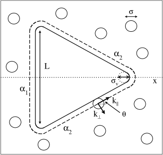
Figure 1: Sketch of an inelastic equilateral triangle with different coefficient of restitution on left and right side ($\alpha_{1}$ and $\alpha_{2}$ respectively) and surrounding by a gas of inelastic particles. The dashed line correspond to the effective triangle seen by a colliding disk.

In this case the outer surface is $\tilde{C}=3L+\pi(\sigma+\sigma_{v})$ where $L$ is the “linear” side of the triangle (see Fig. 1). The function $F(\theta)$, using the symmetry of the object, becomes

$$F(\theta)= \frac{L}{\tilde{C}}\Big{[}\delta\Big{(}\theta-\frac{3}{2}\pi\Big{)}+2\delta\Big{(}\theta-\frac{\pi}{6}\Big{)}\Big{]}+\frac{r_{e}}{\tilde{C}}$$ (26)

with $r_{e}=(\sigma+\sigma_{v})/2$.
Moreover, the transition rate (8) can be written as

$$W(V|V^{\prime})= n\tilde{C}\sqrt{\frac{m}{2\pi T_{g}}}\Big{[}(V^{\prime}-V)\Theta(V^{\prime}-V)g_{-}(V,V^{\prime})+$$ (27)

$$(V-V^{\prime})\Theta(V-V^{\prime})g_{+}(V,V^{\prime})$$

where

$$g_{-}(V,V^{\prime}) =\int_{\sin\theta>0}d\theta F(\theta)\frac{\kappa^{2}(\theta,\alpha_{2})}{\sin^{2}\theta}\cdot$$ (28)

$$\exp\Big{\{}-\frac{m\sin^{2}\theta}{2T_{g}}\left[\frac{\kappa(\theta,\alpha_{2})}{\sin^{2}\theta}(V-V^{\prime})+V^{\prime}\right]^{2}\Big{\}}\equiv$$

$$\equiv\int_{\sin\theta>0}d\theta F(\theta)~{}\lambda(\theta,\alpha_{2},V,V^{\prime})$$

$$g_{+}(V,V^{\prime}) =\int_{\sin\theta<0}d\theta F(\theta)~{}\lambda(\theta,\alpha_{1},V,V^{\prime}).$$ (29)

The last line of Eq. (28) defines the function $\lambda(\theta,\alpha(\theta),V,V^{\prime})$. Using the Eq. (26) and the symmetry respect to $\theta$, the above expressions become

$$g_{-}(V,V^{\prime}) =\frac{2L}{\tilde{C}}\lambda\left(\frac{\pi}{6},\alpha_{2},V,V^{\prime}\right)+\frac{r_{e}}{\tilde{C}}\int_{0}^{\pi}\!\!\!\!d\theta~{}\lambda(\theta,\alpha_{2},V,V^{\prime})$$ (30)

$$g_{+}(V,V^{\prime}) =\frac{L}{\tilde{C}}\lambda\left(\frac{\pi}{2},\alpha_{1},V,V^{\prime}\right)+\frac{r_{e}}{\tilde{C}}\int_{0}^{\pi}\!\!\!\!d\theta~{}\lambda(\theta,\alpha_{1},V,V^{\prime})$$ (31)

Some sections of the transition rate surface, for different values of $\epsilon^{2}$, are shown in Fig. 2, together with the simulation data obtained from a DSMC with $\tau_{b}/\tau_{dd}=137.5$ and $\alpha_{dd}=0.9$.

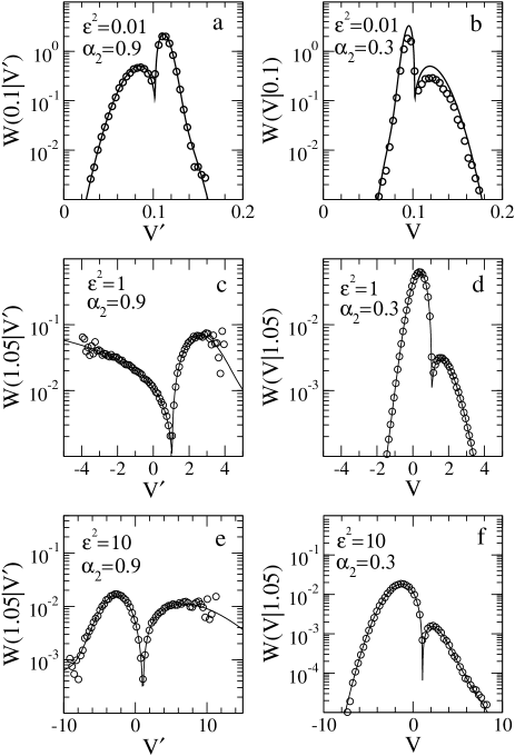
Figure 2: The transition rate $W(V|V^{\prime})$ of an inelastic equilateral triangle for different values of the mass ratio $\epsilon^{2}$ and the coefficient of restitution $\alpha_{2}$. The panels a, c and e show the trend as a function of $V^{\prime}$ for $\alpha_{2}=0.9$, $\alpha_{dd}=0.9$ and $\epsilon^{2}=0.01,1$ and $10$ respectively. The panels b, d and f instead show the trend as a function of $V$ for $\alpha_{2}=0.3$ and for the same values of $\epsilon^{2}$. The symbols correspond to the simulation data, while the lines are obtained from Eqs.(27) and (30)-(31).

The Figure 2 displays a very good agreement between theory and DSMC for the transition rate for all values of $\alpha_{2}$ and $\epsilon^{2}$ studied.
In Fig. 3 we show the rescaled observable $\langle V\rangle/V_{th}$ as a function of the right coefficient of restitution $\alpha_{2}$ for different values of $\epsilon^{2}$. The theory results in good agreement with the simulation data, supporting our assumptions. The trends are analogue to those obtained in [7], where only the inelasticity asymmetry was considered: such a similarity indicates that the effects, due to the different inelasticity of the ratchet, are predominant with respect to the geometrical asymmetry, that however can be not neglected [5]. The data referring to ratio $\eta$ of the granular temperatures of the system go in the same direction (see Fig. 4).

5 Conclusion

Within the present article we have investigated the statistical properties of a specific non equilibrium system, a 2D object sliding along an axis and colliding inelastically with a granular gas coupled to a thermal bath. If the object has an asymmetric shape or possesses a non uniform inelasticity profile, one observes a net drift. It is possible, employing the BE, to describe theoretically the system. We first obtain the collision frequency between ratchet and disks. Such a quantity determines the interplay between the gas and the ratchet dynamics. Secondly, we have derived a system of coupled equations of some relevant averages of the distribution functions of the ratchet and of the gas, respectively, describing the time evolution of the whole system. In the limit of light objects ($\epsilon^{2}\ll 1$), it is fundamental to include the third moment of the ratchet in order to attain a satisfactory description of the ratchet behavior. We have performed DSMC simulations in the case of an equilateral triangle and compared the theoretical predictions with the numerical results and found a fair agreement: in particular, we have measured the transition rate of the tracer, its mean velocity and the granular temperature for difference $\epsilon^{2}$ values. Whereas the theory gives an explicit representation of such transition rates based on the assumption of a Maxwellian velocity distribution for the gas particles, our simulations give a direct estimate of the same quantity. The good agreement with the analytic results confirms our assumptions.

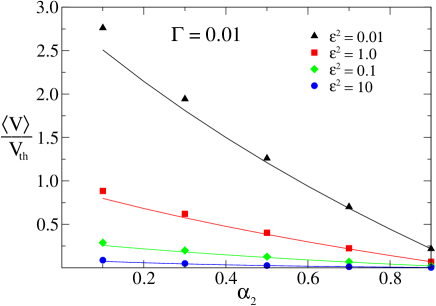
Figure 3: The velocity of an equilateral triangle ratchet, rescaled with its thermal velocity $V_{th}=\sqrt{T_{r}/M}$, as function of the coefficient of restitution $\alpha_{2}$ for $\alpha_{dd}=0.9$, $\tau_{b}/\tau_{dd}=137.5$ and for different values of the parameter $\epsilon^{2}$: $10$ (circles), $1.0$ (squares), $0.1$ (diamonds) and $0.01$ (triangles). The symbols correspond to the simulation data while the lines correspond to the solutions obtained from Eqs.(15)-(20).

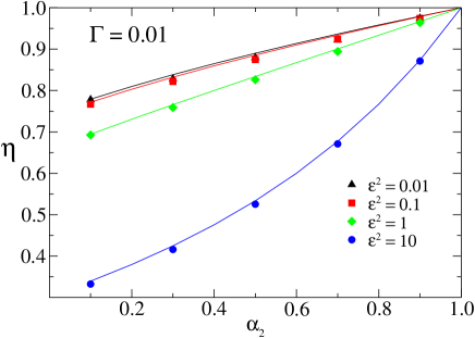
Figure 4: The temperature ratio $\eta=T_{r}/T_{g}$ as function of the coefficient of restitution $\alpha_{2}$ for the same cases of Fig. 3. The symbols correspond to the simulation data while the lines correspond to the solutions obtained from Eqs.(15)-(20).

Appendix

The coefficients of the Eq.(14) and Eqs. (15)-(17) can be written as

$$u_{1}(z)=\int_{0}^{2\pi}d\theta F(\theta)\sqrt{z+\sin^{2}\theta}$$

$$u_{2}(z)=\int_{0}^{2\pi}d\theta F(\theta)\frac{\sin^{4}\theta}{(z+\sin^{2}\theta)^{3/2}}$$

$$u_{3}(z)=\int_{0}^{2\pi}d\theta F(\theta)\frac{\sin^{3}\theta\cos\theta}{(z+\sin^{2}\theta)^{3/2}}$$

$$a_{1}(z)=\int_{0}^{2\pi}d\theta F(\theta)\frac{\sin\theta}{1+\epsilon^{2}\sin^{2}\theta}(1+\alpha(\theta))\left(z+\sin^{2}\theta\right)$$

$$a_{2}(z)=\int_{0}^{2\pi}d\theta F(\theta)\frac{\sin^{2}\theta}{1+\epsilon^{2}\sin^{2}\theta}(1+\alpha(\theta))\sqrt{z+\sin^{2}\theta}$$

$$a_{3}(z)=\int_{0}^{2\pi}d\theta F(\theta)\frac{\sin\theta\cos\theta}{1+\epsilon^{2}\sin^{2}\theta}(1+\alpha(\theta))\sqrt{z+\sin^{2}\theta}$$

$$a_{4}(z)=\int_{0}^{2\pi}d\theta F(\theta)\frac{(1+\alpha(\theta))\sin^{4}\theta}{(1+\epsilon^{2}\sin^{2}\theta)\sqrt{z+\sin^{2}\theta}}$$

$$b_{1}(z)=\int_{0}^{2\pi}d\theta F(\theta)\frac{(1+\alpha(\theta))\epsilon^{4}\sin^{2}\theta}{(1+\epsilon^{2}\sin^{2}\theta)^{2}}\sqrt{z+\sin^{2}\theta}\left[z(1+\alpha(\theta))+\sin^{2}\theta(\alpha(\theta)-1)-2\right]$$

$$b_{2}(z)=\int_{0}^{2\pi}d\theta F(\theta)\frac{\sin\theta}{(1+\epsilon^{2}\sin^{2}\theta)^{2}}\Big{\{}3(1+\alpha(\theta))^{2}z\epsilon^{4}\sin^{2}\theta+\left[1-(2+3\alpha(\theta))\epsilon^{2}\sin^{2}\theta\right]\cdot$$

$$(1-\alpha(\theta)\epsilon^{2}\sin^{2}\theta)\Big{\}}$$

$$b_{3}(z)=\int_{0}^{2\pi}d\theta F(\theta)\frac{\cos\theta}{(1+\epsilon^{2}\sin^{2}\theta)^{2}}\Big{\{}3(1+\alpha(\theta))^{2}z\epsilon^{4}\sin^{2}\theta+\left[1-(2+3\alpha(\theta))\epsilon^{2}\sin^{2}\theta\right]\cdot$$

$$(1-\alpha(\theta)\epsilon^{2}\sin^{2}\theta)\Big{\}}$$

$$b_{4}=\int_{0}^{2\pi}d\theta F(\theta)\frac{\sin\theta}{(1+\epsilon^{2}\sin^{2}\theta)^{2}}\left(1-\alpha(\theta)\epsilon^{2}\sin^{2}\theta\right)^{2}$$

$$b_{5}(z)=\int_{0}^{2\pi}d\theta F(\theta)\frac{\sin^{2}\theta}{(1+\epsilon^{2}\sin^{2}\theta)^{2}(z+\sin^{2}\theta)^{5/2}}\Big{\{}6z^{2}(1-\alpha(\theta)\epsilon^{2}\sin^{2}\theta)^{2}+z\sin^{2}\theta\cdot$$

$$\Big{[}12(1+\alpha(\theta))^{2}\epsilon^{4}\sin^{4}\theta+5(1+\epsilon^{2}\sin^{2}\theta)\left(1+\epsilon^{2}\sin^{2}\theta-4(1+\alpha(\theta))\epsilon^{2}\sin^{2}\theta\right)\Big{]}$$

$$+2\sin^{4}\theta(1-\alpha(\theta)\epsilon^{2}\sin^{2}\theta)\Big{[}1-(2+3\alpha(\theta))\epsilon^{2}\sin^{2}\theta\Big{]}-(1+\epsilon^{2}\sin^{2}\theta)^{2}\cdot$$

$$(6z^{2}+5z\sin^{2}\theta+2\sin^{4}\theta)\Big{\}}$$

$$b_{6}(z)=\int_{0}^{2\pi}d\theta F(\theta)\frac{\sin\theta\cos\theta}{(1+\epsilon^{2}\sin^{2}\theta)^{2}(z+\sin^{2}\theta)^{5/2}}\Big{\{}6z^{2}(1-\alpha(\theta)\epsilon^{2}\sin^{2}\theta)^{2}+z\sin^{2}\theta\cdot$$

$$\Big{[}12(1+\alpha(\theta))^{2}\epsilon^{4}\sin^{4}\theta+5(1+\epsilon^{2}\sin^{2}\theta)\left(1+\epsilon^{2}\sin^{2}\theta-4(1+\alpha(\theta))\epsilon^{2}\sin^{2}\theta\right)\Big{]}$$

$$+2\sin^{4}\theta(1-\alpha(\theta)\epsilon^{2}\sin^{2}\theta)\Big{[}1-(2+3\alpha(\theta))\epsilon^{2}\sin^{2}\theta\Big{]}-(1+\epsilon^{2}\sin^{2}\theta)^{2}\cdot$$

$$(6z^{2}+5z\sin^{2}\theta+2\sin^{4}\theta)\Big{\}}$$

$$c_{1}(z)=\int_{0}^{2\pi}d\theta F(\theta)\frac{\sin\theta}{(1+\epsilon^{2}\sin^{2}\theta)^{3}}\Big{\{}(1+\alpha(\theta))^{3}z^{2}\epsilon^{6}\sin^{2}\theta+(1+\alpha(\theta))z\epsilon^{2}\Big{[}1-(1+2\alpha(\theta))\cdot$$

$$\epsilon^{2}\sin^{2}\theta\Big{]}(1-\alpha(\theta)\epsilon^{2}\sin^{2}\theta)-(1-\alpha(\theta)\epsilon^{2}\sin^{2}\theta)^{3}\Big{\}}$$

$$c_{2}(z)=\int_{0}^{2\pi}d\theta F(\theta)\frac{\sin^{2}\theta}{(1+\epsilon^{2}\sin^{2}\theta)^{3}(z+\sin^{2}\theta)^{3/2}}\Big{\{}8z^{3}\epsilon^{6}\sin^{2}\theta(1+\alpha(\theta))^{3}+6z^{2}\epsilon^{2}\Big{[}1+\alpha(\theta)-$$

$$(1+\alpha(\theta))(1+3\alpha(\theta))\epsilon^{2}\sin^{2}\theta+(1+\alpha(\theta))(2+5\alpha(\theta)+4\alpha^{2}(\theta))\epsilon^{4}\sin^{4}\theta\Big{]}+$$

$$z\Big{[}(1+2\alpha(\theta))\epsilon^{2}\sin^{2}\theta-1\Big{]}^{3}+2\sin^{2}\theta(1-\alpha(\theta)\epsilon^{2}\sin^{2}\theta)[(3+4\alpha(\theta))\epsilon^{2}\sin^{2}\theta-$$

$$1]-(1+\epsilon^{2}\sin^{2}\theta)^{3}\left(3z+2\sin^{2}\theta\right)\Big{\}}$$

$$c_{3}(z)=\int_{0}^{2\pi}d\theta F(\theta)\frac{1}{(1+\epsilon^{2}\sin^{2}\theta)^{3}(z+\sin^{2}\theta)^{5/2}}\Big{\{}2z^{3}(1-\alpha(\theta)\epsilon^{2}\sin^{2}\theta)^{2}[1-(3+4\alpha(\theta))\cdot$$

$$\epsilon^{2}\sin^{2}\theta]+z^{2}\sin^{2}\theta\Big{[}15-5(1+10\alpha(\theta))\epsilon^{2}\sin^{2}\theta+5(1+4\alpha(\theta)-12\alpha^{2}(\theta))\cdot$$

$$\epsilon^{4}\sin^{4}\theta+(1-2\alpha(\theta)-12\alpha^{2}(\theta)-24\alpha^{3}(\theta))\epsilon^{6}\sin^{6}\theta\Big{]}+2z\sin^{4}\theta\Big{[}10-(1+$$

$$31\alpha(\theta))\epsilon^{2}\sin^{2}\theta+(1+4\alpha(\theta)-33\alpha^{2}(\theta))\epsilon^{4}\sin^{4}\theta-\alpha(\theta)(1+3\alpha(\theta)+12\alpha^{2}(\theta))\cdot$$

$$\epsilon^{6}\sin^{6}\theta\Big{]}+8\sin^{6}\theta(1-\alpha(\theta)\epsilon^{2}\sin^{2}\theta)^{3}-(1+\epsilon^{2}\sin^{2}\theta)^{3}\Big{[}2z^{3}+15z^{2}\sin^{2}\theta+$$

$$20z\sin^{4}\theta+8\sin^{6}\theta\Big{]}\Big{\}}$$

$$c_{4}=\int_{0}^{2\pi}d\theta F(\theta)\frac{\sin\theta}{(1+\epsilon^{2}\sin^{2}\theta)^{3}}(1-\alpha(\theta)\epsilon^{2}\sin^{2}\theta)^{2}\left[1-(3+4\alpha(\theta))\epsilon^{2}\sin^{2}\theta\right]$$

$$c_{5}(z)=\int_{0}^{2\pi}d\theta F(\theta)\frac{\epsilon^{2}\sin^{2}\theta}{(1+\epsilon^{2}\sin^{2}\theta)^{3}\left(z+\sin^{2}\theta\right)^{3/2}}\Big{\{}8z^{3}(1+\alpha(\theta))^{3}\sin^{2}\theta+6z^{2}(1+\alpha(\theta))\cdot$$

$$\Big{[}1-(1+3\alpha(\theta))\epsilon^{2}\sin^{2}\theta+(2+5\alpha(\theta)+4\alpha^{2}(\theta))\epsilon^{4}\sin^{4}\theta\Big{]}+6z(1+\alpha(\theta))\sin^{2}\theta\cdot$$

$$\Big{[}3-6\alpha(\theta)\epsilon^{2}\sin^{2}\theta+(1+2\alpha(\theta)+4\alpha^{2}(\theta)\epsilon^{4}\sin^{4}\theta\Big{]}+2\sin^{4}\theta\Big{[}6(1+\alpha(\theta))+$$

$$3(1+\alpha(\theta))(1-3\alpha(\theta))\epsilon^{2}\sin^{2}\theta+(1+3\alpha^{2}(\theta)+4\alpha^{3}(\theta))\Big{]}\Big{\}}$$

$$c_{6}(z)=\int_{0}^{2\pi}d\theta F(\theta)\frac{\epsilon^{2}\sin\theta\cos\theta}{(1+\epsilon^{2}\sin^{2}\theta)^{3}\left(z+\sin^{2}\theta\right)^{3/2}}\Big{\{}8z^{3}(1+\alpha(\theta))^{3}\sin^{2}\theta+6z^{2}(1+\alpha(\theta))$$

$$\Big{[}1-(1+3\alpha(\theta))\epsilon^{2}\sin^{2}\theta+(2+5\alpha(\theta)+4\alpha^{2}(\theta))\epsilon^{4}\sin^{4}\theta\Big{]}+6z(1+\alpha(\theta))\sin^{2}\theta\cdot$$

$$\Big{[}3-6\alpha(\theta)\epsilon^{2}\sin^{2}\theta+(1+2\alpha(\theta)+4\alpha^{2}(\theta))\epsilon^{4}\sin^{4}\theta\Big{]}+2\sin^{4}\theta\Big{[}6(1+\alpha(\theta))+$$

$$3(1+\alpha(\theta))(1-3\alpha(\theta))\epsilon^{2}\sin^{2}\theta+(1+3\alpha^{2}(\theta)+4\alpha^{3}(\theta))\Big{]}\Big{\}}$$

$$c_{7}=\int_{0}^{2\pi}d\theta F(\theta)\frac{\sin\theta}{(1+\epsilon^{2}\sin^{2}\theta)^{3}}\Big{[}1-3(1+2\alpha(\theta))\epsilon^{2}\sin^{2}\theta+3\alpha(\theta)(2+3\alpha(\theta))\epsilon^{4}\sin^{4}\theta-$$

$$\alpha^{2}(\theta)(3+4\alpha(\theta))\epsilon^{6}\sin^{6}\theta\Big{]}$$

$$c_{8}=\int_{0}^{2\pi}d\theta F(\theta)\frac{\cos\theta}{(1+\epsilon^{2}\sin^{2}\theta)^{3}}\Big{[}1-3(1+2\alpha(\theta))\epsilon^{2}\sin^{2}\theta+3\alpha(\theta)(2+3\alpha(\theta))\epsilon^{4}\sin^{4}\theta-$$

$$\alpha^{2}(\theta)(3+4\alpha(\theta))\epsilon^{6}\sin^{6}\theta\Big{]}$$

$$d_{1}(z)=\int_{0}^{2\pi}d\theta F(\theta)\frac{\cos\theta}{1+\epsilon^{2}\sin^{2}\theta}(1+\alpha(\theta))\left(z+\sin^{2}\theta\right)$$

$$d_{2}(z)=\int_{0}^{2\pi}d\theta F(\theta)\frac{(1+\alpha(\theta))\cos^{2}\theta}{1+\epsilon^{2}\sin^{2}\theta}\sqrt{z+\sin^{2}\theta}$$

$$d_{3}(z)=\int_{0}^{2\pi}d\theta F(\theta)\frac{(1+\alpha(\theta))\sin^{3}\theta\cos\theta}{(1+\epsilon^{2}\sin^{2}\theta)\sqrt{z+\sin^{2}\theta}}$$

$$e_{1}(z)=\int_{0}^{2\pi}d\theta F(\theta)\frac{1+\alpha(\theta)}{1+\epsilon^{2}\sin^{2}\theta}\sqrt{z+\sin^{2}\theta}\left[z(\alpha(\theta)-1-2\epsilon^{2}\sin^{2}\theta)+(1+\alpha(\theta))\sin^{2}\theta\right]$$

$$e_{2}(z)=\int_{0}^{2\pi}d\theta F(\theta)\frac{\sin\theta}{(1+\epsilon^{2}\sin^{2}\theta)^{2}}\Big{\{}3(1+\alpha(\theta))^{2}\sin^{2}\theta+z\Big{[}2(1+\epsilon^{2}\sin^{2}\theta)^{2}+(1+\alpha(\theta))\cdot$$

$$(3\alpha(\theta)-1-4\epsilon^{2}\sin^{2}\theta)\Big{]}\Big{\}}$$

$$e_{3}(z)=\int_{0}^{2\pi}d\theta F(\theta)\frac{\cos\theta}{(1+\epsilon^{2}\sin^{2}\theta)^{2}}\Big{\{}3(1+\alpha(\theta))^{2}\sin^{2}\theta+z\Big{[}2(1+\epsilon^{2}\sin^{2}\theta)^{2}+(1+\alpha(\theta))\cdot$$

$$(3\alpha(\theta)-1-4\epsilon^{2}\sin^{2}\theta)\Big{]}\Big{\}}$$

$$e_{4}=\int_{0}^{2\pi}d\theta F(\theta)\frac{(1+\alpha(\theta))^{2}\sin^{3}\theta}{(1+\epsilon^{2}\sin^{2}\theta)^{2}}$$

$$e_{5}(z)=\int_{0}^{2\pi}d\theta F(\theta)\frac{(1+\alpha(\theta))\sin^{4}\theta}{(1+\epsilon^{2}\sin^{2}\theta)^{2}(z+\sin^{2}\theta)^{5/2}}\Big{[}z^{2}(5+3\alpha(\theta)+2\epsilon^{2}\sin^{2}\theta)+2z\sin^{2}\theta\cdot$$

$$(4+3\alpha(\theta)+\epsilon^{2}\sin^{2}\theta)+3(1+\alpha(\theta))\sin^{4}\theta\Big{]}$$

$$e_{6}(z)=\int_{0}^{2\pi}d\theta F(\theta)\frac{(1+\alpha(\theta))\sin^{3}\theta\cos\theta}{(1+\epsilon^{2}\sin^{2}\theta)^{2}(z+\sin^{2}\theta)^{5/2}}\Big{[}z^{2}(5+3\alpha(\theta)+2\epsilon^{2}\sin^{2}\theta)+2z\sin^{2}\theta\cdot$$

$$(4+3\alpha(\theta)+\epsilon^{2}\sin^{2}\theta)+3(1+\alpha(\theta))\sin^{4}\theta\Big{]}$$

References

References

- [1] Hanggi P and Marchesoni F, Artificial Brownian motors: Controlling transport on the nanoscale 2009 Rev. Mod. Phys. 81 387
- [2] Van den Broeck C, Kawai R and Meurs P, Microscopic Analysis of a Thermal Brownian Motor, 2004 Phys. Rev. Lett. 93 090601
- [3] Meurs P, Van den Broeck C and Garcia A, Rectification of thermal fluctuations in ideal gases, 2004 Phys. Rev. E 70 051109
- [4] Pöschel T and Luding S 2001 Granular Gases, Lecture Notes in Physics (Springer, Berlin)
- [5] Costantini G, Marini Bettolo Marconi U and Puglisi A, Granular Brownian ratchet model, 2007 Phys. Rev. E 75 061124
- [6] Cleuren B and Van den Broeck C, Granular Brownian motor, 2007 Europhys. Lett. 77 50003
- [7] Costantini G, Marini Bettolo Marconi U and Puglisi A, Noise rectification and fluctuations of an asymmetric inelastic piston, 2008 Europhys. Lett. 82 50008
- [8] Puglisi A, Loreto V, Marini Bettolo Marconi U, Petri A and Vulpiani A, Clustering and non-Gaussian behavior in granular matter, 1998 Phys. Rev. Lett. 81 3848; Puglisi A, Loreto V, Marini Bettolo Marconi U and Vulpiani A, A kinetic approach to granular gases, 1999 Phys. Rev. E 59 5582
- [9] Bird G A 1994 Molecular Gas Dynamics and the Direct Simulation of Gas Flows (Clarendon Oxford); Montanero J M and Santos A, Computer simulation of uniformly heated granular fluids, 2000 Granular Matter 2 53
- [10] Cecconi F, Diotallevi F, Marini Bettolo Marconi U and Puglisi A, Fluid-like behavior of a one-dimensional granular gas, 2004 J. Chem. Phys.120 35; Cecconi F, Marini Bettolo Marconi U, Diotallevi F Puglisi A, Inelastic hard rods in a periodic potential, 2004 J. Chem. Phys. 121 5125
- [11] Williams D R M and MacKintosh F C, Driven granular media in one dimension: Correlations and equation of state, 1996 Phys. Rev. E 54 R9 - R12; van Noije T P C , Ernst M H, Velocity distributions in homogeneously cooling and heated granular fluids, 1998 Granular Matter 1 57-64; Pagonabarraga I, Trizac E, van Noije T C P, Ernst M H, Randomly driven granular fluids: Collisional statistics and short scale structure, 2001 Phys Rev E 65 011303
- [12] Garzó V and Montanero J M, Transport coefficients of a heated granular gas, 2002 Physica A 313 336-356
- [13] Risken H 1984 The Fokker-Planck Equation. Methods of Solution and Applications (Springer Series in Synergetics, Springer-Verlag, Berlin - Heidelberg - New York - Tokyo), Vol. 18
- [14] Sela N and Goldhirsch I, Hydrodynamics of a one-dimensional granular medium, 1995 Phys. Fluids 7 507
- [15] Puglisi A, Visco P, Trizac E and van Wijland F, Dynamics of a tracer granular particle as a non-equilibrium markov process, 2006 Phys. Rev. E 73 021301