Two-component jet simulations: Combining analytical and numerical approaches

Abstract

Recent observations as well as theoretical studies of YSO jets suggest the presence of two steady components: a disk wind type outflow needed to explain the observed high mass loss rates and a stellar wind type outflow probably accounting for the observed stellar spin down. In this framework, we construct numerical two-component jet models by properly mixing an analytical disk wind solution with a complementary analytically derived stellar outflow. Their combination is controlled by both spatial and temporal parameters, in order to address different physical conditions and time variable features. We study the temporal evolution and the interaction of the two jet components on both small and large scales. The simulations reach steady state configurations close to the initial solutions. Although time variability is not found to considerably affect the dynamics, flow fluctuations generate condensations, whose large scale structures have a strong resemblance to observed YSO jet knots.

1 Introduction

In the last few years, a promising two-component jet scenario seems to emerge in order to explain Young Stellar Object (YSO) outflows. Observational data of Classical T Tauri Stars (CTTS) Edw06 , Kwa07 indicate the presence of two genres of winds: one being ejected radially with respect to the central object and the other being launched at a constant angle with respect to the equatorial plane (e.g. Tzeferacos et al., this volume). In turn, CTTS outflows may be associated with either a stellar origin, or a disk one or with both wind components having roughly equivalent contributions. In addition, such a scenario is supported by theoretical arguments as well (e.g. Fer06 ). An extended disk wind is required for the explanation of the observed YSO mass loss rates, whereas a pressure driven stellar outflow is expected to propagate in the central region, being a strong candidate to address the protostellar spin down Mat08 .

The goal of the present work is to study the two-component jet scenario, taking advantage of both analytical and numerical approaches. In particular, we construct numerical models by setting as initial conditions a mixture of two analytical YSO outflow solutions (each one describing a disk or a stellar jet), ensuring the dominance of the stellar component in the inner regions and of the disk wind in the outer. The combination is achieved with the introduction of few normalization and mixing parameters, along with enforced time variability of the stellar component. We investigate the evolutionary properties, steady states and the features of the final configurations of the dual component jets. Although the detailed launching mechanisms of each component are not taken into account, such models seem capable to capture the dynamics and describe a variety of interesting scenarios.

The employed analytically derived MHD outflows, defined as ADO (Analytical Disk Outflow; denoted with subscript D) and ASO (Analytical Stellar Outflow; denoted with subscript S), have been derived in the context of self-similarity Vla98 and each one effectively describes a disk wind Vla00 or a stellar jet Sau02 , respectively. In Matsakos et al. Tit08 , we have addressed the topological stability, as well as several physical and numerical properties, separately for each solution. This article summarizes the numerical setup and reports the results of few significant cases of the dual component jet. A thorough study can be found in Matsakos et al. Titsu .

2 Numerical two-component jet models

The two-component jet model parameters can be classified in two categories. The first one contains those associated to the relative normalization of the analytical solutions, i.e. the ratios of the characteristic scales of each model (denoted with subscript *, calculated on a specific fieldline at the Alfvénic surface):

$$\ell_{L}=\frac{R_{*}}{r_{*}}\,,\quad\ell_{V}=\frac{V_{S*}}{V_{D*}}\,,\quad\ell_{B}=\frac{B_{S*}}{B_{D*}}\,,$$ (1)

where $R_{*}$ is the Alfvénic spherical radius of the ASO model, $r_{*}$ is the cylindrical radius of the Alfvénic surface of the ADO model (of a specific fieldline) and the subscripts $L$, $V$ and $B$ stand for length, velocity and magnetic field, respectively. We assume that the protostar has a solar mass and a radius of $\sim 0.01\,AU$. Since the disk wind launching region lies in the range $0.2-3\,$AU, we derive $\ell_{L}=0.1$ and $\ell_{V}=5.96$. On the other hand, we define $\ell_{B}=2$, which is the parameter controlling the relative dominance of each model.

The second class of parameters concerns the mixing. In particular, we choose the combination to depend on the magnetic flux function $A$, which labels the fieldlines of each analytical model ($A_{D}$ or $A_{S}$). Therefore, we define a common trial magnetic flux $A_{tr}=A_{D}+A_{S}$ and then all physical variables $U$ are initialized with the help of the following mixing function:

$$U_{2comp}=\left\{1-\exp\left[-\left(\frac{A_{tr}}{qA_{m}}\right)^{d}\right]\right\}U_{D}+\exp\left[-\left(\frac{A_{tr}}{qA_{m}}\right)^{d}\right]U_{S}\,,$$ (2)

where $A_{m}$ is a constant corresponding to the matching surface rooted at $0.16\,$AU, $q$ is a parameter that effectively moves this surface closer to the protostar and $d$ sets the steepness of the transition from the inner ASO to the outer ADO solution. We choose $q=0.2$ and $d=2$, whereas a complete parameter study (including $\ell_{B}$) can be found in Titsu . Essentially, Eq. 2 provides an exponential damping of each solution around a particular fieldline of the combined magnetic field.

Moreover, since accretion and protostellar variability are expected to introduce fluctuations we multiply the inflow velocity with the following function:

$$f_{S}(r,t)=1+\frac{1}{2}\sin\left(\frac{2\pi t}{T_{var}}\right)\exp\left[-\left(\frac{r}{2r_{m}}\right)^{2}\right]\,,$$ (3)

where $T_{var}$ is the period of the pulsation and $r_{m}$ is roughly the cylindrical radius at which the matching surface intersects the lower boundary of the computational box. Outflow variability produces the formation of knot-like structures: the introduction of radiation cooling (Tesileanu et al. this volume) will allow direct comparison with observational data.

The simulations are performed with PLUTO (Mignone et al. Mig07 ). A uniform resolution of 256 zones for every $100\,$AU is used whereas the simulations have been carried out up to a final time of $80\,$y. On the lower boundary we keep fixed all variables to their initial values, on the axis we apply axisymmetric boundary conditions and at the upper and right borders of the domain we prescribe outflow conditions.

3 Results

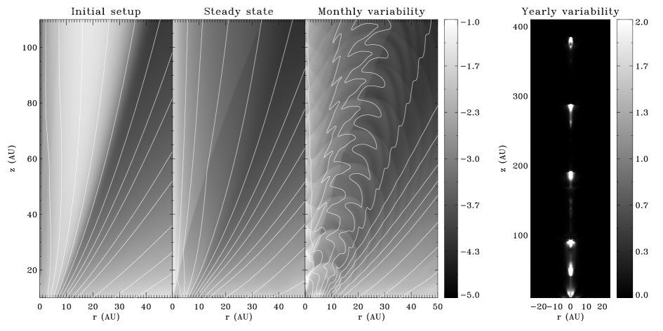
Figure 1: Left panel: Logarithmic density contours (the code unit is $10^{-12}\,$g cm^-3) and magnetic fieldlines for the initial two-component jet model (left), final steady state (middle) and when a monthly flow variability is applied (right). Right panel: The quantity $10^{3}\rho^{2}\sqrt{T}$ (roughly related with emissivity) is plotted for the yearly variable model. Although $\max(10^{3}\rho^{2}\sqrt{T})=53.9$, the color bar uses a lower maximum value to enhance the displayed features.

In the left panel of Fig. 1, the initial setup (left) and the final configuration (middle) of the two-component jet are displayed. The model shows remarkable stability and reaches a well defined steady state in only a few years. In particular, the disk wind solution remains almost unmodified whereas the stellar component gets compressed around the axis. Moreover, a shock manifests during time evolution, located roughly along the diagonal line which crosses (10, 40) and (30, 100) (steady state plot). This shock is found to causally disconnect the acceleration regions from the jet propagation physics and the subsequent interaction with the outer medium. Note that there is no such “horizon” present in the initial setup. Furthermore, on the right plot of the left panel of Fig. 1, the same model is displayed when a monthly time variable velocity is applied on the lower boundary (Eq. 2). Evidently, despite the strong gradients seen in the density and the wiggling of the magnetic fieldlines, the general structure is retained, proving the stability of the two-component jet model.

The fact that the system remains very close to the initial configuration, demonstrates that the analytical solutions provide solid foundations for realistic two-component jet scenarios. Consequently, specific YSO systems can be addressed more accurately by constructing analytical outflow solutions with the desirable characteristics, before merging them into a two-component regime.

On the right panel of Fig. 1 a quantity related to emissivity is plotted in larger scales when a yearly variability is applied. Near the base, the numerical solution remains close to the initial ADO and ASO models. However, farther away along the flow the fluctuations create knot-like structures, which may be related with jet variability. In fact, note that the model is associated with a condensations spacing $\sim 100\,$AU, similar to the knot spacing of HH30.

Finally, although not presented in this article, an other important parameter is the one controlling the relative contribution of each component, $\ell_{B}$, with which we can effectively and smoothly switch the model from a totally magneto-centrifugal wind to a pressure driven jet Titsu .

4 Conclusions

To sum up (taking also into account the results of Tit08 and Titsu ), most of the technical part concerning two-component jets, e.g. 2.5D stability, steady states, parameter study, time variability etc., is now at hand Titsu , providing us with all the necessary ingredients to address YSO jets. Namely, with a) the proper analytical solutions, i.e. desirable lever arm, mass loss rate etc., b) the correct choice of the mixing parameters and c) an enforced time variability that effectively produces knot structures, we are now ready to qualitatively study different and realistic scenarios, address observed jet properties and ultimately understand the various outflow phases of specific T Tauri stars.

- (1) Edwards, S., Fischer, W., Hillenbrand, L., & Kwan, J., ApJ, 646, 319–341 (2006)
- (2) Ferreira, J., Dougados, C., & Cabrit, S., A&A, 453, 785–796 (2006)
- (3) Kwan, J., Edwards, S., & Fischer, W., ApJ, 657, 897–915 (2007)
- (4) Matsakos, T., Tsinganos, K., Vlahakis, N., Massaglia, S., Mignone, A., & Trussoni, E., A&A, 477, 521–533 (2008)
- (5) Matsakos, T., Tsinganos, K., Vlahakis, N., Massaglia, S., Trussoni, E., Sauty, C. & Mignone, A., submitted to A&A.
- (6) Matt, S., & Pudritz, R., ApJ, 678, 1109–1118 (2008)
- (7) Mignone, A., Bodo, G., Massaglia, S., Matsakos, T., Tesileanu, O., Zanni, C., & Ferrari, A., ApJS, 170, 228–242 (2007)
- (8) Sauty, C., Trussoni, E., & Tsinganos, K., A&A, 389, 1068–1085 (2002)
- (9) Vlahakis, N., & Tsinganos, K., MNRAS, 298, 777–789 (1998)
- (10) Vlahakis, N., Tsinganos, K., Sauty, C., & Trussoni, E., MNRAS, 318, 417–428 (2000)