Generalizing Unweighted Network Measures to Capture the Focus in Interactions

Abstract

Unweighted network measures are commonly used to analyze real-world networks due to their simplicity and intuitiveness. This motivated the search for generalizations of unweighted network measures that take weights into account. We propose a new generalization methodology that capture how focused are the interactions over edges. The less focused the interaction (more uniform over edges) the closer is our generalization to the original unweighted measure. None of the previously developed generalizations capture this aspect of weighted networks. We analyze several real world networks using our generalizations of the degree and the clustering coefficient. The analysis shows that our generalizations reveal interesting observations.

1 Introduction

Mining and analyzing complex networks have received significant attention in recent years due to the explosive growth of social networks and the discovery of common patterns that govern wide-range of real world networks watts98n ; barabasi99s ; faloutsos99sigcomm ; chakrabarti06acs ; newman06phr ; clauset07arxiv ; park07pnas . The core of mining complex networks is network measures. Network measures are functions that summarize the network structure to simpler numeric values. These measures are generally classified into two main classes: measures that ignore edge weights and focus primarily on the structure of the graph, which we call unweighted measures, and measures that take edge weights into account (in addition to the structure), which we call weighted measures.

Unweighted measures received the bulk of researchers’ attention, due to their simplicity, intuitiveness, and the relative ease of computation. Such an attention resulted in several influential findings such as the small world (relied on the clustering coefficient) watts98n and the power-law (relied on the degree distribution)barabasi99s ; clauset07arxiv . Despite their popularity, unweighted measures ignore important network information: the weights. Consequently, several measures were developed in order to take weights into account. The use of weighted measures, however, is still dwarfed by the use of unweighted measures in analyzing complex networks boccaletti06pr ; leskovec07atkdd ; clauset07arxiv ; park07pnas .

The wide spread usage of unweighted network measures motivated the search for generalizations of unweighted measures that takes weights into account barrat04pnas ; ahnert07pre ; opsahl09sn ; opsahl10sn . For example, one generalization of the degree computed the expected number of edges incident to a node, assuming the weight of an edge reflects the probability of the edge existing ahnert07pre . The most recent generalization of the degree measure used a tunable parameter $\alpha$ to mix both the unweighted degree and the strength using simple multiplication opsahl10sn . Section 5 describes in more detail the previous generalizations and the related work.

We propose in this paper a new generalization methodology that captures the degree of focus of interaction. If the interaction is not focused and uniform over edges (uniform weights), then our generalized measure reduces to the original unweighted measure (and this reduction is guaranteed). So for example, if a node has five neighbors and it interacts with all five neighbors equally (no focus), then our generalization of the degree reports the node to have a generalized degree of 5, similar to the unweighted degree. If the node focuses and limits its interaction with only two out of five neighbors, then our generalization of the degree will capture this focus and report the node to have a generalized degree closer to 2 rather than 5.

Consider the simplified scenario in Figure 1[a] for illustration. Four students met for the first time in some class. Initially all of the four students are interacting uniformly with one another, forming a clique with equal edge weights. The weight attached to a link (edge) between two students quantifies the amount of interaction between the two students. As time passes, each student focuses her interaction on fewer subset of students (friends). As a result, some links get weaker and eventually disappear, while other links get stronger. The final interaction network shows lesser average degree.

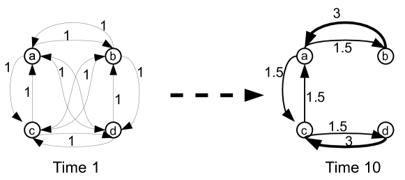
Figure 1: A simplified scenario of a dynamic network. The figure shows the evolution of interaction among 4 students in a class. In the beginning (Time 1) every student interacts with every other student equally (every weight equals 1). As time passes, some links get weaker while other links get stronger. At the end (Time 10), only subset of links have weight greater than 0, and not all the weights are equal.

Now suppose we monitor the evolution of edge weights over time at different snapshots. For simplicity, suppose the weights of different edges increase (or decrease) linearly from Time 1 to Time 10. So for example, the edge from node $a$ to node $b$ increases by a rate of $0.05$ per time unit. Similarly, the edge from node $c$ to node $b$ decreases by a rate of $-0.1$ per time unit. Notice here that the amount of out-ward interaction of each node (the strength) remains constant over time (and equal 3). However, out-ward interaction becomes focused towards 2 or less neighbors. Figure 2 shows the corresponding evolution of the degree distribution, the strength distribution, and the $\alpha$-degree distribution for two values of $\alpha$: 0.5 and 1.5 opsahl10sn . Notice that neither the strength nor the $\alpha$-degree reflects the degree distribution of the final network at Time 10. Furthermore, none of the measures capture the change in the focus of interaction over time. In other words, although the change in the interaction pattern between students was gradual, this gradual change is not captured by any of the measures (instead, there is a sudden jump in the distribution).

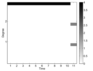
(a) Degree Distribution

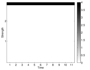
(b) Strength Distribution

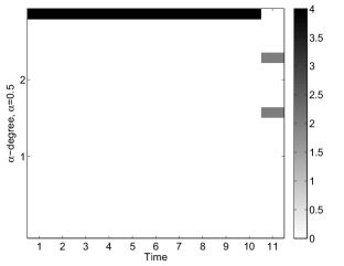
(c) $\alpha$-Degree Distribution, $\alpha=0.5$

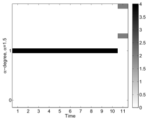
(d) $\alpha$-Degree Distribution, $\alpha=1.5$

Figure 2: The corresponding evolution of common network measures for the students dynamic network: the degree distribution, the strength distribution, and the $\alpha-$degree distribution for $\alpha=0.5$ and $\alpha=1.5$. Two issues here are worth noting: (1) neither the strength nor the $\alpha$-degree reflects the degree distribution of the final network at Time 10 (2) None of the measures capture the change of interaction focus in a gradual continuous manner.

Figure 3 shows the evolution of our degree generalization for the student network scenario. Notice here the continuity of our measure (Figure 3[b]), in contrast to the unweighted degree. Notice also that when there at Time 1 and Time 10, our generalized degree is identical to the original unweighted degree.

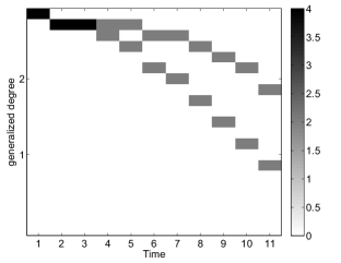
(a) C-Degree Distribution

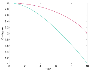
(b) C-degree evolution

Figure 3: The corresponding evolution of our generalization of the degree measure, the continuous-degree (C-degree) for the students dynamic network: the degree distribution. Part (a) shows the histogram of the C-degree over time, discretized into 20 bins. Part(b) shows the C-degree for the four nodes over finer time-scale. Notice the continuous evolution of our generalization and the direct connection to the unweighted degree at the beginning and at the end of the timescale.

We illustrate the applicability of our method by generalizing four unweighted measures: the node degree, the clustering coefficient, the dyadicity, and the heterophilicity. As a case study, we analyze several real-world, weighted, social networks using two generalized measures: the C-degree and the C-clustering coefficient (the letter C stands for continuous and denotes our generalization of an unweighted measure).

But before we describe our contribution in the following section, it is important to state the limitations and the assumptions of our approach. We assume that an edge’s weight reflects the amount of interaction across that edge, which is a reasonable assumption in most real-world domains. For example, an edge weight can represent the number of times a person calls a friend, the number of emails transmitted to an email address, or the number of papers co-authored by two scientists. On the other hand, if weights reflect something like the dissimilarity between neighbors, then our approach is not suitable. More importantly, our generalization captures the focus of interactions not the intensity of the interactions. For example, suppose that in the previous student network scenario we multiply the weights (over all edges) by some constant every time step (instead of adding or subtracting). In this case, both the degree and the C-degree (our generalization) will not change, but the strength and the $\alpha$-degree will change.

The following section describes the heart of our approach: generalizing the cardinality concept of a set to take weights into account.

2 Generalizing Measures Using Generalized Cardinality

Several unweighted measures use the cardinality (the size) of some subset of edges in their computation. For example, the node degree is the number of edges incident to a node. The clustering coefficient of a node is the ratio between the number of edges between its neighbors and the number of all possible edges among the neighbors. The main limitation of the traditional cardinality function (and consequently all the unweighted network measures that use it) is that it ignores edge weights. We show in this section how to generalize the cardinality to capture the focus in interactions. In the following section we show how to use the generalized cardinality to generalize the degree, the clustering coefficient and other unweighted measures that use the cardinality of some edge set.

To put it more formally, let $E^{\prime}=\{e_{1},...,e_{n}\}\subseteq E$ be the subset of edges that are used in computing a particular network measure, where $E$ is the set of all network edges and the cardinality of $E^{\prime}=n=|E^{\prime}|$. The degree of node $i$ is then defined as $k(i)=|E^{\prime}_{i}|$, where $E^{\prime}_{i}$ is the set of edges incident to node $i$. Similarly, the clustering coefficient of node $i$ is $z(i)=\frac{|E^{\prime}_{i}|}{MAX^{N}_{i}}$, where $E^{\prime}_{i}$ here is the set of edges between node $i$’s neighbors and $MAX^{N}_{i}$ is a constant that equals the maximum number of edges that can exist between these neighbors (i.e. if node $i$’s neighbors formed a clique). In weighted networks, each edge $e\in E$ has a corresponding non-negative weight $w(e)\geq 0$. The cardinality implicitly assumes uniform weights over the edges. When weights are not uniform, the cardinality can give an incorrect perception of the actual use of edges. Consider the following numeric example. There are four sets of edges with corresponding multisets of weights $W_{1}=\{5,5,5,5\},W_{2}=\{9,5,5,1\},W_{3}=\{9,8,2,1\}$ and $W_{4}=\{20,0,0,0\}$. The cardinalities of these weight multisets are all the same and equals 4. Intuitively, however, if the weights reflect the interaction over edges, then not all the edges are being used equally and the traditional cardinality becomes a crude approximation. It is possible to define a cutoff threshold weight (an edge is included in the graph if its weight is above a threshold, otherwise the edge is excluded). The computation of any unweighted measure then takes place naturally chapanond05cmot ; kalisky06phr . Such an approach, however, does not properly handle the focus of interaction among neighbors, and it is not clear how big or small should the threshold be.

Instead, we want a generalized cardinality function that summarizes a set of weighted edges into a single real number and has two properties. If edge weights are equal (no focus), then the function we are looking for should return the traditional cardinality. When the weights are not equal, the function should assign a value between 1 and the traditional cardinality such that the more equal the weights are (less focus), the higher the value. The two properties ensure the consistent connection between the original measure and the generalization. The second property ensures that the generalized measure captures the degree of focus in interactions. Using the previous numeric example, we are looking for a function that assigns 4 to $W_{1}$, 1 to $W_{4}$, and values between 1 and 4 for $W_{2}$ and $W_{3}$, with the value assigned to $W_{2}$ greater than the value assigned to $W_{3}$ (because the two inner weights are equal in case of $W_{2}$). Such a generalization of the cardinality measure will allow straightforward generalization of many unweighted network measures.Simple functions for summarizing sets (such as the average, the variance, and the summation) can be very useful in summarizing weights, but they do not satisfy the two desired properties mentioned above.

The heart of our generalization is a generalized definition of the cardinality of a set of edges $E^{\prime}$ that takes weights into account, which we call the effective cardinality, or $c(E^{\prime})$:

$$c(E^{\prime})=\left\{\begin{array}[]{ll}0&\textrm{if $E^{\prime}$ is empty}\\ 2^{\left(\sum_{e\in E^{\prime}}\frac{w(e)}{\sum_{o\in E^{\prime}}w(o)}\log_{2}\frac{\sum_{o\in E^{\prime}}w(o)}{w(e)}\right)}&otherwise\end{array}\right.$$

Intuitively, the quantity $\frac{w(e)}{\sum_{o\in E^{\prime}}w(o)}$ represents the probability of an interaction over an edge $e$ among all the edges in $E^{\prime}$. The multiset $\left\{\frac{w(e)}{\sum_{o\in E^{\prime}}w(o)}:e\in E^{\prime}\right\}$ is a probability distribution over edges and $H(E^{\prime})=\sum_{e\in E^{\prime}}\left[\frac{w(e)}{\sum_{o\in E^{\prime}}w(o)}\log_{2}\frac{\sum_{o\in E^{\prime}}w(o)}{w(e)}\right]$ is the entropy of this probability distribution. The entropy measures the disparity between the weights: the more uniform the weights are, the higher the entropy and vice versa. The purpose of the power 2 is to convert the entropy back to the number of edges that are effectively being used. In other words, the effective cardinality of edge set $E^{\prime}$ returns the number of edges of equal weights that has the same entropy as the edges in $E^{\prime}$.

Before discussing the important properties of the effective cardinality, let us first consider few numeric examples that illustrate the intuition. Consider the multiset of weights $W=\{10,0.01\}$. The traditional cardinality of this set is 2. However, if weights quantify the amount of interaction over edges, then the interaction is highly focused over one edge and the cardinality should be closer to 1 than 2. For $W=\{10,0.01\}$, $c(\{10,0.01\})=1.008$, so even though the set $W$ has two edges, the effective cardinality is equivalent to only $1.008$. For the numeric example we have mentioned earlier, $c(W_{1}=\{5,5,5,5\})=4$, $c(W_{2}=\{9,5,5,1\})=3.3276$, $c(W_{3}=\{9,8,2,1\})=3.0219$ and $W_{4}=\{20,0,0,0\}=1$, which satisfy the intuitive ordering we described earlier. This ordering is not just by chance or due to a special case, but is actually guaranteed by our proposed effective cardinality.

The effective cardinality satisfies three properties (proofs follow from entropy properties and are given in the appendix):

1. Preserving maximum cardinality: $\forall E^{\prime}:c(E^{\prime})\leq|E^{\prime}|$. Furthermore, $c(E^{\prime})=|E^{\prime}|$ iff $\forall e\in E^{\prime}:w(e)=C$, where $C$ is some constant. In other words, the effective cardinality is maximum and equals the original cardinality when there is no disparity between weights.

2. Preserving minimum cardinality: $c(E^{\prime})=0$ iff $E^{\prime}$ is an empty set. Furthermore, $c(E^{\prime})=1$ iff $\exists u\in E^{\prime}:w(u)>0$ and $\forall v\neq u:w(v)=0$. In other words, the effective cardinality is one when all edges, except one edge, have zero weights.

3. Consistent partial order over weighted sets: any function that maps a set of real numbers (weights) to a single real number imposes an implicit partial order. The effective cardinality imposes, arguably, the simplest partial order that is consistent with the above two properties. If the two sets of weighted edges have the same size, the same summation of weights, and their individual weights are the same except for two edges, then the set with more uniform weights has higher effective cardinality (a formal definition of this property is given in Lemma 3 in the appendix).

The three properties ensure a consistent connection to the original cardinality. The properties also confirm that the effective cardinality (and consequently any generalized measure based on it) captures and is sensitive to the focus of interaction (the disparity between weights). The effective cardinality, however, is not sensitive to the scale of weights. So for example, the multiset of weights $\{1,1\}$ has the same effective cardinality as the multiset $\{10,10\}$. This can be contrasted to the traditional degree, which is sensitive to neither the scale nor the disparity, and the strength, which is not sensitive to the disparity of weights but is sensitive to the scale. We come back to this issue in our analysis in Section 4. The following section uses the effective cardinality to generalize some unweighted measures.

3 Generalizing Unweighted Network Measures Using Effective Cardinality

In principal, unweighted network measures which use the cardinality of some subset of edges can be generalized using the effective cardinality. In fact, while we limited the discussion in the previous section to sets of weighted edges, all discussed properties apply to any multiset of weights, even if elements in the set represent subgraphs, not edges. So for example, if we are interested in counting triangles of three connected vertices (which are used in some definitions of the clustering coefficient), we can use the effective cardinality to replace the discrete count of triangles with a continuous spectrum. This section presents four example generalizations of unweighted network measures: the degree, the clustering coefficient, the dyadicity, and the heterophilicity. The resulting generalized measures inherit the three properties of the effective cardinality. Table 1 summarize these generalizations.

Measure	Unweighted	Generalized
Degree of node $i$	$|E_{i}|$	$c(E_{i})$
Clustering coefficient of node $i$	$\frac{|E^{N}_{i}|}{MAX^{N}_{i}}$	$\frac{c(E^{N}_{i})}{MAX^{N}_{i}}$
Dyadicity of a graph	$\frac{|E_{within}|}{n_{within}}$	$\frac{c(E_{within})}{n_{within}}$
Heterophilicity of a graph	$\frac{|E_{across}|}{n_{across}}$	$\frac{c(E_{across})}{n_{across}}$

Table 1: The summary of the generalization of four unweighted measures, where $E_{i}$ is the set of edges incident to node $i$, $E^{N}_{i}$ is the set of edges between neighbors of node $i$, $E_{within}$ is the set of edges within a class of nodes, and $E_{across}$ is the set of edges across two classes of nodes.

The dyadicity and heterophilicity were recently used to study the correlation between the types of nodes (node classes) and the network structure park07pnas . The dyadicity of a graph equals $\frac{|E_{within}|}{n_{within}}$, where $E_{within}$ is the set of edges within a set of nodes of the same type (a class of nodes) and $n_{within}$ is the expected number of edges within the same class of nodes if there was no correlation between the node class and the network structure. Intuitively, the dyadicity quantifies the strength of connections between nodes of the same type and whether it is above average. The heterophilicity of a graph equals $\frac{|E_{across}|}{n_{across}}$, where $E_{across}$ is the set of edges across two classes of nodes and $n_{across}$ is the expected number of edges across the two classes if there was no correlation between the node class and the network structure. The heterophilicity quantifies the strength of connections across two classes (communities) of nodes and whether it is above average. The dyadicity can be generalized, using the effective cardinality, to be $\frac{c(E_{within})}{n_{within}}$ and similarly the heterophilicity can be generalized to be $\frac{c(E_{across})}{n_{across}}$.

The degree and the clustering coefficient, of a particular node, are two of the most widely used unweighted measures, so the remainder of this section focuses on their generalization.

3.1 Generalizing the Degree

A node’s degree is the number of edges incident to the node, or $|E_{i}|$, where $E_{i}$ is the set of edges incident to node $i$. The degree distribution (the histogram of the degrees of all network nodes), has been used extensively to analyze and characterize networks, and helped in discovering common patterns in real world networks, particularly the power law barabasi99s ; faloutsos99sigcomm ; boccaletti06pr ; clauset07arxiv ; leskovec07atkdd . A degree distribution follows the power law if $P(k)\propto k^{-\alpha}$, where $k$ is the degree, $\alpha$ is a constant, and $P(k)$ is the degree distribution. A generalization of the degree measure using the effective cardinality, which we call the continuous degree (C-degree), is straightforward:

Definition 1

The C-degree of a node $i$ in a network is $r(i)$, where

$$r(i)=c(E_{i})=\left\{\begin{array}[]{ll}0&\textrm{if $i$ is disconnected}\\ 2^{\left(\sum_{e\in E_{i}}\frac{w(e)}{s(i)}\log_{2}\frac{s(i)}{w(e)}\right)}&otherwise\end{array}\right.$$

The set $E_{i}$ is the set of edges incident to node $i$ and $s(i)=\sum_{e\in E_{i}}w(e)$ is the strength of node $i$. Figure 4 compares the continuous degree distribution to the (discrete) degree distribution in a simple weighted network of four nodes. A node on the boundary has an out degree of 1, while an internal node has an out degree of 2. Intuitively, however, only one of the internal nodes is fully utilizing its degree of 2 (the one to the left), while the other node (to the right) is mostly using one neighbor only. The C-degree measure captures this and shows that the internal node to the left has a C-degree of $c(\{0.5,0.5\})=2$ while the other internal node has a C-degree of $c(\{0.9,0.1\})=2^{H(0.9,0.1)}=1.38$.

Figure 4: Example weighted network of four nodes, comparing the (discrete) degree against the C-degree. The degree distribution illustrates the benefit of taking weights into account in distinguishing nodes.

The C-degree inherits the three properties we described earlier with respect to the traditional node degree. The C-degree of a node is maximum and equals the traditional discrete degree when all the weights incident to the node are equal. The C-degree of a connected node is minimum and equals one if all edges incident to the node have zero weights except one edge that has a weight greater than zero. And finally, everything else being equal, a node with more uniform weights incident to it (less focused interaction) has higher C-degree than a node with less uniform weights incident to it.

3.2 Generalizing the Clustering Coefficient

The clustering coefficient is a measure that quantifies the clustering or connectivity among a node’s neighbors. When averaged over all nodes, the clustering coefficient represents the connectivity of the whole network. The clustering coefficient is an important property for identifying small world networks watts98n and is given by the equation $\frac{|E_{i}^{N}|}{MAX_{i}^{N}}$, where $E_{i}^{N}$ is the set of edges between node $i$’s neighbors and $MAX^{N}_{i}$ is the maximum number of edges that can be between these neighbors. The generalized clustering coefficient of a node $i$ using the effective cardinality is:

$$o(i)=\frac{c(E_{i}^{N})}{MAX_{i}^{N}}$$

Figure 5 provides a simple motivating example of 3-nodes. The C-clustering coefficient can help in distinguishing different nodes that are deemed indistinguishable using the traditional clustering coefficient. For example, both nodes $A$ and $B$ have a clustering coefficient of $2/2=1$ (neighboring nodes have two edges between them, out of two possible edges). However, $B$’s C-clustering coefficient is $o(B)=c(\{5,1\})/2=0.78$, while the C-clustering coefficient of $A$ is $o(A)=c(\{5,5\})/2=1$.

Figure 5: Example weighted network of three nodes, comparing the (discrete) clustering coefficient against the C-clustering coefficient. The scatter plot of the degree against the clustering coefficient illustrates the benefit of taking weights into account in distinguishing nodes.

4 Experimental Verification

The previous sections provide theoretical analysis as to why our method maintains a connection to the original measures, captures the focus of interaction, and translates that to a continuous spectrum of values. However, several important questions remain unanswered: in a realistic large network, will the proposed generalization be of value? Will it provide more information than the original unweighted measures? Will the generalized measures still maintain connection to their original unweighted measures?

We conduct three types of experimental evaluations (in addition to the theoretical analysis provided earlier) to show the potential of our method: analyzing snapshots of real-world networks (similar to most of the previous workahnert07pre ; opsahl09sn ; opsahl10sn ), analyzing the evolution of a semi-realistic dynamic weighted network, and analyzing the informativeness of our generalization when used to predict labels of network nodes.

4.1 Analysis of Network Snapshots

We have analyzed four real world weighted networks that capture coauthorships between scientists. Three of which were extracted from preprints on the E-Print Archive newman01pnas : condensed matter (an updated version of the original dataset that includes data between Jan 1, 1995 and March 31, 2005), astrophysics, and high-energy theory. The fourth network represents coauthorship of scientists in network theory and experiment newman06phr . The weight between two scientists $i$ and $j$ reflects the strength of their collaboration and is given by the equation $w_{ij}=\sum_{m}{\frac{\delta_{i}^{m}\delta_{j}^{m}}{n_{m}-1}}$, where $\delta_{i}^{m}=1$ if scientist $i$ was a co-author of paper $m$ and $n_{m}$ is the number of co-authors for paper $m$newman01pre . Table 2 summarize some statistics about the datasets.

Dataset key	astro-ph	netscience	cond-mat	hep-th
num of nodes	16706	1589	40421	8361
num of edges	121251	2742	175693	15751
Weights STD	0.515	0.427	0.889	1.175

Table 2: Statistics of the network datasets

Figure 6 displays the C-degree distribution (CDD) and the (discrete) degree distribution (DD) for the four collaboration network. The figure uses log-log scale with the power law fit based on clauset07arxiv . The CDD follows a pattern similar to the DD, despite taking weights into account. However, the power-law fit for the CDD has steeper decline (higher $\alpha$) than the DD. As the degree of a scientist increases, the scientist interacts with a smaller subset of neighbors. While this observation is expected, it raises an interesting question: does the size expected of this collaboration subset remain stable? In other words, on average, does a highly connected scientist collaborates primarily with $X$ number of other scientists, regardless of her degree? or will the number $X$ be a function of the scientist’s degree? To answer this question, we define the degree utilization metric as the ratio between the C-degree and the degree of a node: $u(v)=\frac{r(v)}{k(v)}$. The degree utilization measures the focus of interaction as a percentage of the original degree. Figure 7 plots the degree utilization against the (discrete) degree for the four collaboration networks. A common pattern emerges in the four networks. For low degrees, the degree utilization is relatively high: scientists with few collaborators rarely focus on subset of these collaborators. For nodes with degree greater than some constant the collaboration becomes focused and the degree utilization drops. However, and to our surprise, a cone is observed, which starts wide at low degrees and gets narrower as the degree increases (the average degree utilization is plotted as a line in the figure). A scientist focuses on a number of collaborators that, on average, is a percentage of the total number of collaborators. This percentage differs from one discipline to another.

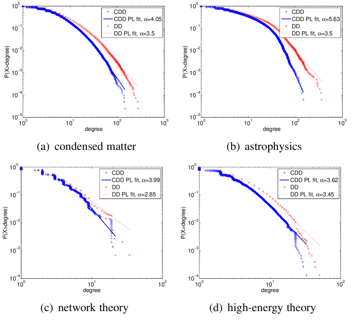
Figure 6: Comparing the discrete degree distribution (DD) with the continuous degree distribution (CDD) for the four collaboration networks. The power law fit (PL fit) is also shown with the associated power.

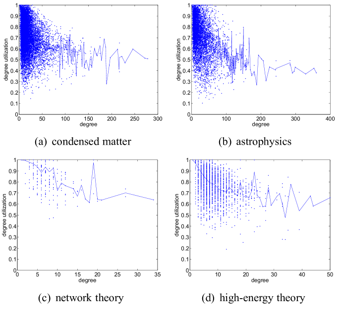
Figure 7: Scatter plot of a node degree against its degree utilization for the four collaboration networks. the average utilization per degree is also plotted.

Figure 8 shows the scatter plot of the (discrete) clustering coefficient versus the (discrete) degree (shown in log scale) for the four collaboration networks. The main observation clear from the graph is that in general, the clustering coefficient decreases with the increase of the degree. In other words, the higher the number of collaborators of a scientist, the lesser the density of edges between these collaborators.

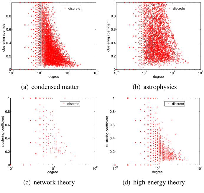
Figure 8: Scatter plot of a node’s discrete degree against its discrete clustering coefficient for the four collaboration networks.

Figure 9 shows the scatter plot of the C-clustering coefficient versus the C-degree for the four collaboration networks. The continuous version of the scatter plot follows the general observation in the discrete case: the clustering coefficient decreases with the increase of the degree. Nevertheless, the scatter plot for the continuous measures covers more area, because both the C-degree and the C-clustering coefficient produce continuous spectrum of values (unlike the discrete degree and the discrete clustering coefficient). Note also that due to maximum cardinality property, Figure 9 is shifted towards the origin when compared to Figure 8. More importantly, one can observe an interesting pattern in the continuous scatter plot: nodes with high C-clustering coefficient (above 0.8) tend to have more discrete C-degree. This is clear from the concentration of points with high C-clustering coefficient around the discrete degrees. The same observation is not apparent in points with low clustering coefficient. Using Lemma 1, this observation means that nodes with incident weights that are more uniform (hence the more discrete degree) tend to cluster with nodes that have more uniform weights among themselves (hence the higher clustering coefficient). We believe this observation reflects research groups: scientists forming cliques of collaboration with almost equal weights over edges (most publications are co-authored by research group members).

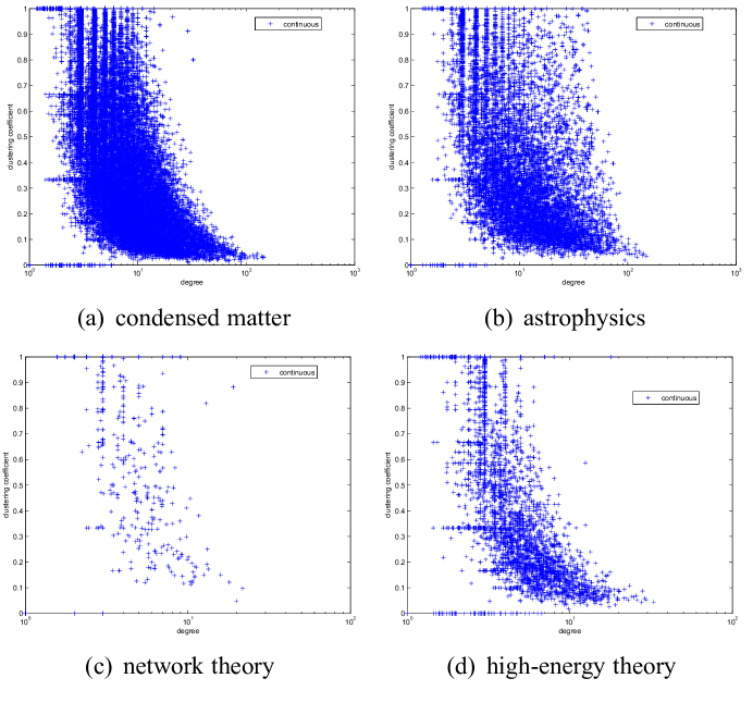
Figure 9: Scatter plot of a node’s continuous degree against its continuous clustering coefficient for the four collaboration networks.

4.2 Analysis Using Node Classification

Recently, researchers discovered that using label-independent network measures can provide useful information in classifying network nodes gallagher09snakdd . We follow this direction in this section. First, we compute for each node 5 label-independent features: the (discrete) degree, the C-degree, the strength, the clustering coefficient, and the C-clustering coefficient. Then we apply different feature selection algorithms to assess the importance of different features. Each feature selection algorithm selects a subset of features based on some criteria. The criteria differ from one feature selection algorithm to another, but usually takes into account the correlation between a feature (or subset of features) and the node’s label.

We studied 6 labeled datasets, 4 of which represent university websites (University of Texas, Cornell University, Washington University, and University of Wisconsin), while the remaining two represent relationships between industrial companies extracted from news articles (according to two studies). Table 3 shows some statistics about the 6 datasets: number of nodes, number of links, the percentage of weights that are equal one, and the standard deviation of weights. From the table, we can see that majority of weights equal one for all datasets (ranging from 60% to almost 80%), but the Washing. and the Ind-yh datasets have significantly lower percentage (and consequently more variety in weights).

Data set key	Texas	Cornell	Washing.	Wiscon.	Ind-pr	Ind-yh
num of nodes	338	351	434	354	2189	1798
num of edges	32988	2683	30462	33250	13062	14165
% of weights=1	0.74	0.76	0.6	0.79	0.75	0.64
Weights STD	1.47	1.34	2.93	3.18	2.46	10.81

Table 3: Statistics of the labeled network datasets

As mentioned earlier, 5 features are computed for each node: the degree (D), the clustering coefficient (C), the C-degree (CD), the C-clustering coefficient (CC), and the strength (S). The strength is added here to capture the impact of scale, which is ignored by the first 4 features. Given these features, the idea is to apply feature selection algorithms and observe for each dataset which features are considered significant or more important than others. Since different algorithms may select different features, more than one algorithm were applied. We focus here on publicly available algorithms through the WEKA software package, using the default settings weka09 . We also avoid algorithms that discretize features, because discretizing a continuous generalization diminishes its advantage.

Table 4 shows the outcome of applying the first feature selection algorithm: CfsSubsetEval weka09 . The algorithm outputs a subset of features that have high correlation with the class and low correlation among themselves. As the table shows, the C-degree was selected in 5 of the 6 datasets, compared to only 4 datasets where the degree was selected. It is interesting to note here that the only dataset where the C-degree was not selected (Ind-pr), the degree was not selected as well. On the other hand, the strength was selected in that dataset, which means that for Ind-pr dataset and the CfsSubsetEval algorithm, the class is more correlated with the scale rather than the degree of focus. It is interesting to observe here that although the strength measure takes weights into account, the degree is still more informative. This observation explains why the degree is still widely used in analyzing weighted networks. Also the C-clustering coefficient was selected in 3 datasets, while the original clustering coefficient was selected only once.

Texas	Cornell	Washing	Wiscon	Ind-pr	Ind-yh
CD	CD	CD	CD	CC	CD
D	D	D	D	C
CC	C	CC		S
	S

Table 4: Selected features using CfsSubsetEval

Table 5 shows the results of another feature selection algorithm: ClassifierSubsetEval with 1-nearest neighbor classifier. The algorithm evaluates subsets of attributes using the accuracy of the 1-nearest neighbor classifier to prefer one subset over the other. As shown in the table, this feature selection algorithm confirms a clear advantage to our approach. None of the original unweighted measures was selected for any dataset. Unlike the previous feature selection algorithm, however, the C-clustering seems to be more dominant across datasets (selected in all of them). Interestingly, the strength was selected in 5 out of the 6 datasets, complementing the disparity sensitivity with the scale sensitivity for this particular feature selection algorithm.

Texas	Cornell	Washing	Wiscon	Ind-pr	Ind-yh
CC	CD	CD	CD	CD	CC
S	CC	CC	CC	CC	S
	S	S		S

Table 5: Selected features subset using ClassifierSubsetEval with 1-nearest neighbor classifier

Table 6 shows the numerical ranking for the features using the ReliefFAttributeEval algorithm. The algorithm evaluates each attribute by repeatedly sampling an instance and considering the value of the attribute for the nearest instances of the different classes. To simplify comparison, the values for each dataset was divided by the maximum value of the column (higher is better). From the table we can see that the C-degree always has higher value than the original degree. It is interesting to note that the difference is highest (Ind-yh and Washing) in datasets with less percentage of weights equal 1 (Table 3). The C-clustering coefficient was better than the traditional clustering coefficient in 4 datasets, and worse in 2 datasets. Interestingly, the strength has the highest value in the Ind-pr dataset, which is consistent with the results of the previous feature selection algorithm (as discussed earlier regarding Table 5, Ind-pr is the only dataset where neither the C-degree not the degree was selected).

Feature	Texas	Cornell	Washing	Wiscon	Ind-pr	Ind-yh
CD	1	1	0.884	1	0.808	1
D	0.925	0.999	0.780	0.989	0.807	0.588
CC	0.633	0.503	1	0.297	0.397	0.553
C	0.547	0.480	0.535	0.145	0.465	0.752
S	0.354	0.395	0.473	0.246	1	0.248

Table 6: Selected features subset using the ReliefFAttributeEval algorithm

4.3 Analysis of Dynamic Networks

We believe our methodology will be most effective in studying the evolution of weighted networks over time. Unfortunately, we were not able to find any publicly available dataset that provided such an evolution. Most of the available datasets of weighted networks provided only snapshots of a particular network at a particular point in time. The other possibility is to synthesize the evolution of a weighted network. Several models were proposedli07pa . However, all these models were designed to capture the properties that are known (e.g. power-law of degree distribution and/or the power-law of the strength distribution) and are less helpful in evaluating new measures. We opted for a simpler alternative: growing the weights of some initial network to eventually be equivalent to a publicly-available network snapshot. More formally: let $N_{last}$ be some snapshot of a real world network (e.g. the science collaboration network). Let $N_{0}$ be some initial network that has the same structure as $N_{last}$ but with different initial weights. We then developed two simple mechanisms to evolve a network from $N_{0}$ to $N_{last}$.

• Assuming initially all weights are zero, increase the weight of every edge proportional to the edge’s weight in $N_{last}$.

• Assuming initially the interaction for each node is not focused (i.e. all weights are equal), while maintaining the same strength, change the weights gradually in the direction of $N_{last}$.

Figure 10 shows the evolution of the our generalized degree distribution for each mechanism using the netscience collaboration network. As expected, our generalization captures the change in the focus of interaction properly, while other measures fail. When there is no change in the focus, our generalization remains unchanged.

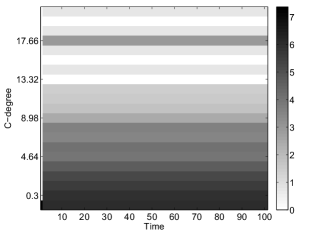
(a) Changing scale

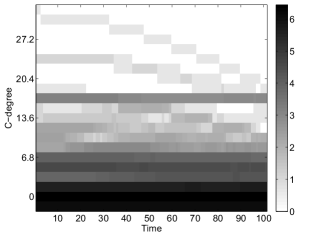
(b) Changing focus

Figure 10: The evolution of the netscience networks under two simple mechanisms: changing the scale and changing the focus. As expected, our generalization captures the change in the focus properly, while other measures fail. When there is no change in the focus, our generalization remains unchanged. Note that the frequency (the gray scale) is in log scale.

5 Related Work

In general, one can classify weighted network measures into two classes: measures that generalize unweighted network measures to take weights into account, and measures that have no connection to unweighted measures. Surveying all weighted measures that have no connection to unweighted measures is beyond the scope of this paper and have little relevance to the contribution of this paper, which generalizes unweighted network measures. For completeness, we provide here a sample of these measures that are related to some unweighted measure (interested reader may refer to survey papers on the subject newman04preA ; barth05pa ; boccaletti06pr ). The strength of a node is the summation of all weights incident to a node. The strength becomes identical to the node’s degree in the very special case when all the weights are equal to 1, but it has very weak partial ordering among nodes. For example, all the nodes in Figure 4 have the same strength of 1. The weight distribution is similar to the degree distribution except that it measures the frequency of a particular edge weight. A more recent work mcglohon08kdd analyzed a graph’s total weight, $\sum_{e\in E}w(e)$, against the graph’s total number of edges, $|E|$, over time. That work also analyzed the degree of a node, $k(v)$, against the node’s strength, $s(v)$. While useful, the above measures neither captured the degree of focus in interactions nor provided a methodology for generalizing unweighted measures, unlike our proposed generalization. The network measure $Y(v)=\sum_{e\in E(v)}\left(\frac{w(e)}{s(v)}\right)^{2}$ successfully captured the disparity of interaction within edges incident to node $v$ almaas04n . However, unlike our work here, the $Y$ measure is not a generalization of the degree measure.

There have been several attempts to generalize specific unweighted measures. The weighted clustering coefficient barrat04pnas was an attempt to generalize the clustering coefficient. The generalization relied on an alternative definition of the clustering coefficient that used triplets watts98n . A triplet connected to a node is a subgraph containing the original node in addition to two other connected neighbors. The intuition behind the weighted clustering coefficient for node $i$ is to weigh every edge between two of its neighbors, $j$ and $k$, using the weights on edges $(i,j)$ and $(i,k)$. However, unlike our generalization, the weight on edge $j,k$ was ignored. A recent attempt to generalize the clustering coefficient used the ratio between the total value of closed triplets and the total value of all triplets opsahl09sn . The authors proposed four functions to evaluate (summarize) weighted triplets: the arithmetic mean, the geometric mean, the minimum, and the maximum. The four proposed functions (and therefore the proposed generalization) have weaker distinguishing powers than our proposed method. For example, all the nodes in Figure 5 will have a generalized clustering coefficient of 1 if the method in opsahl09sn is used (this limitation was previously reported opsahl09sn ). On the other hand, our proposed generalized clustering coefficient successfully distinguishes all the three nodes.

The ensemble approach ahnert07pre provides a methodology for generalizing almost all unweighted network measures. The first step of the method was to normalize edge weights to ensure all weights are between 0 and 1 (more restrictive than our approach, which only assumes weights are non-negative). The next step was to randomly generate an ensemble of unweighted networks from the original weighted network, where the weight of an edge represented the probability of generating the edge. The final step was to compute the generalized unweighted measure as the average of the unweighted measure for each network in the ensemble. Because the ensemble approach relies on computing the expectation, the method could not provide any partial ordering guarantee. For example, suppose two nodes have the following sets of incident edge weights $A=\{9,8,2,1\}$ and $B=\{9,5,5,1\}$. Under the ensemble approach, both nodes will have the same generalized degree. Using our proposed generalization, node $B$’s degree is guaranteed to be greater than node $A$’s C-degree by Lemma 3.Another side-effect of relying on the expectation is the limited connection to the original unweighted measures. Only if the weights were normalized such that all weights equaled exactly 1 would the ensemble approach provide generalizations equal to the original unweighted measures.

The most recent attempt to generalize the degree (along with betweenness and closeness) relied on mixing total weights (strength) with the cardinality (degree) opsahl10sn . The generalized degree based on this method is the $\alpha$-degree that we described earlier: $\alpha$-degree = $s^{\alpha}k^{1-\alpha}$. Although the generalization methodology were applied to the betweenness and closeness centrality measures, only the degree generalization was evaluated. More importantly, the generalization has a tuning parameter without clear guidelines regarding how to set it, unlike our methodology which is parameterless. Also the connection to the original unweighted measure does not depend on the weights, but on the tuning parameter (when $\alpha$ equals 0). As a result, the $\alpha$-generalization is not really a generalization, but rather a new class of weighted measures.

6 Conclusion

We proposed a new methodology for generalizing measures of unweighted networks. Our method captures the degree of focus in the interaction over edges, and reduces to the original unweighted measure if the interactions are not focused. We illustrated the applicability of our method by generalizing four unweighted network measures including the degree and the clustering coefficient. We complemented the theoretical analysis of our proposed generalization with the experimental analysis of 3 types of datasets. The analysis of labeled dataset classification showed how feature selection algorithms prefer our generalized measures to the original unweighted measures, across different datasets and different feature selection algorithms. The analysis of un-labeled datasets (collaboration networks) showed that the generalized degree distribution follows a similar pattern to the traditional degree distribution, but with steeper decline (larger exponent of the power-law fit). The analysis exposed scientific research groups and showed that, in expectation, scientists focus their collaboration on fixed percentage, regardless of the number of collaborators.

Due to the large body of research that relied on unweighted measures for analyzing networks, there are several interesting directions for following up on this work. We are currently investigating the use of the C-degree in simple network navigation to replace the degree. We are also investigating the use of the generalized measures to study the evolution of interaction networks.

Appendix A: Proofs of Effective Cardinality Properties

Theorem 6.1

The effective cardinality satisfies the three properties described above: the maximum cardinality, the minimum cardinality, and the consistent partial ordering.

Proof

The proof follows from the following three lemmas.

Lemma 1

The effective cardinality satisfies the maximum cardinality property.

Proof

When all the weights are equal to a constant $C$ we have

$$\forall e\in E^{\prime}:\frac{w(e)}{\sum_{o\in E^{\prime}}w(o)}=\frac{C}{C|E^{\prime}|}=\frac{1}{|E^{\prime}|}$$

We then have

$$c(E^{\prime}) =2^{\sum_{e\in E^{\prime}}\frac{1}{|E^{\prime}|}\log_{2}(|E^{\prime}|)}$$

$$=2^{\log_{2}(|E^{\prime}|)}$$

$$=|E^{\prime}|$$

In other words, both the cardinality and the effective cardinality of a weighted set of edges become equivalent when the weights are uniform. The effective cardinality is also maximum in this case, because the exponent is the entropy of the weight probability distribution, which is maximum when weights are uniform over edges.

Lemma 2

The effective cardinality satisfies the minimum cardinality property.

Proof

When the set of edges is empty, then the effective cardinality is zero by definition. When all weights are zero except only one weight that is greater than zero, then weight probability distribution is deterministic and the entropy is zero, therefore the effective cardinality will be 1.

Lemma 3

The effective cardinality satisfies the consistent partial order property.

Proof

Let $E^{\prime}_{1}$ and $E^{\prime}_{2}$ be two (edge) sets such that $|E^{\prime}_{1}|=|E^{\prime}_{2}|$ (both have the same cardinality). Let $W_{1}$ and $W_{2}$ be the corresponding sets of weights, where $\sum_{e1\in E^{\prime}_{1}}w(e1)=\sum_{e2\in E^{\prime}_{2}}w(e2)=S$ (the total weights are equal). Furthermore, let $|W_{1}\bigcap W_{2}|=n-2,\{w_{11},w_{12}\}=W_{1}-W_{2},\{w_{21},w_{22}\}=W_{2}-W_{1}$, where the ’$-$’ operator is the ”set difference” operator (the two sets share the same weights except for two elements in each set), and $|w_{11}-w_{12}|<|w_{21}-w_{22}|$ (the weights of $W_{1}$ are more uniform than the weights of $W_{2}$). To prove that the effective cardinality satisfies the consistent partial ordering property, we need to prove that $c(E^{\prime}_{1})>c(E^{\prime}_{2})$.

Without loss of generality, we can assume that $w_{11}\geq w_{12}$ and $w_{21}\geq w_{22}$, therefore $w_{11}-w_{12}<w_{21}-w_{22}$. We then have

$$w_{11}+w_{12}=S-\sum_{w\in W_{1}\bigcap W_{2}}w=w_{21}+w_{22}$$

or

$$\frac{w_{11}+w_{12}}{S}=1-\sum_{w\in W_{1}\bigcap W_{2}}\frac{w}{S}=\frac{w_{21}+w_{22}}{S}=L$$

therefore

$$L\geq\frac{w_{21}}{S}>\frac{w_{11}}{S}\geq\frac{L}{2}\geq L-\frac{w_{11}}{S}>L-\frac{w_{21}}{S}$$

where $\frac{w_{12}}{S}=L-\frac{w_{11}}{S}$ and $\frac{w_{22}}{S}=L-\frac{w_{21}}{S}$. Then from Lemma 4 we have $h(L,\frac{w_{11}}{S})>h(L,\frac{w_{21}}{S})$, or

$$-\frac{w_{11}}{S}lg(\frac{w_{11}}{S})-(L-\frac{w_{11}}{S})lg(c-\frac{w_{11}}{S})>$$

$$-\frac{w_{21}}{S}lg(\frac{w_{21}}{S})-(L-\frac{w_{21}}{S})lg(c-\frac{w_{21}}{S})$$

Therefore $H(E^{\prime}_{1})>H(E^{\prime}_{2})$, because the rest of the entropy terms (corresponding to $W_{1}\bigcap W_{2}$) are equal, and consequently $c(E^{\prime}_{1})>c(E^{\prime}_{2})$.

Lemma 4

The quantity $h(C,x)=-x\lg(x)-(C-x)\lg(C-x)$ is symmetric around and maximized at $x=\frac{C}{2}$ for $C\geq x\geq 0$.

Proof

$$h(C,\frac{C}{2}+\delta)=-(\frac{C}{2}+\delta)\lg(\frac{C}{2}+\delta)-(\frac{C}{2}-\delta)\lg(\frac{C}{2}-\delta)=h(C,\frac{C}{2}-\delta)$$

Therefore $h(C,x)$ is symmetric around $c/2$. Furthermore, $h(C,x)$ is maximized when

$$\frac{\partial h(C,x)}{\partial x}=0=-1-\lg x+1+\lg(C-x)$$

or

$$\lg x=\lg(C-x)$$

Therefore $h(C,x)$ is maximized at $x=C-x=\frac{C}{2}$.

References

- (1) Ahnert, S.E., Fink, T.M.A.: Clustering signatures classify directed networks. Phys. Rev. E 78(3), 036,112 (2008). DOI 10.1103/PhysRevE.78.036112
- (2) Ahnert, S.E., Garlaschelli, D., Fink, T.M.A., Caldarelli, G.: Ensemble approach to the analysis of weighted networks. Phys Rev E 76(1) (2007). DOI 10.1103/PhysRevE.76.016101. URL http://dx.doi.org/10.1103/PhysRevE.76.016101
- (3) Almaas, E., Kovacs, B., Vicsek, T., Oltvai, Z.N., Barabasi, A.L.: Global organization of metabolic fluxes in the bacterium, escherichia coli. Nature 427, 839 (2004). URL http://www.citebase.org/abstract?id=oai:arXiv.org:q-bio/04030%01
- (4) Barabasi, A.L., Albert, R.: Emergence of scaling in random networks. Science 286(5439), 509–512 (1999). URL http://view.ncbi.nlm.nih.gov/pubmed/10521342
- (5) Barrat, A., Barthélemy, M., Pastor-Satorras, R., Vespignani, A.: The architecture of complex weighted networks. Proceedings of the National Academy of Science 101, 3747–3752 (2004). DOI 10.1073/pnas.0400087101
- (6) Barthélemy, M., Barrat, A., Pastor-Satorras, R., Vespignani, A.: Characterization and modeling of weighted networks. Physica A 346, 34–43 (2005). DOI 10.1016/j.physa.2004.08.047
- (7) Boccaletti, S., Latora, V., Moreno, Y., Chavez, M., Hwang, D.U.: Complex networks: Structure and dynamics. Phys. Rep. 424, 175–308 (2006). DOI 10.1016/j.physrep.2005.10.009
- (8) Chakrabarti, D., Faloutsos, C.: Graph mining: Laws, generators, and algorithms. ACM Comput. Surv. 38(1), 2 (2006). DOI http://doi.acm.org/http://doi.acm.org/10.1145/1132952.1132954
- (9) Chapanond, A., Krishnamoorthy, M.S., Yener, B.: Graph theoretic and spectral analysis of enron email data. Comp. Math. Organ. Theory 11(3), 265–281 (2005). DOI http://dx.doi.org/10.1007/s10588-005-5381-4
- (10) Clauset, A., Rohilla Shalizi, C., Newman, M.E.J.: Power-law distributions in empirical data. ArXiv e-prints (2007)
- (11) Faloutsos, M., Faloutsos, P., Faloutsos, C.: On power-law relationships of the internet topology. Comput. Commun. Rev. 25, 251–262 (1999)
- (12) Gallagher, B., Eliassi-Rad, T.: Leveraging label-independent features for classification in sparsely labeled networks: An empirical study. In: Lecture Notes in Computer Science: Advances in Social Network Mining and Analysis. Springer (2009)
- (13) Kalisky, T., Sreenivasan, S., Braunstein, L.A., Buldyrev, S.V., Havlin, S., Stanley, H.E.: Scale-free networks emerging from weighted random graphs. Phys. Rev. E 73(2), 025103 (2006). DOI 10.1103/PhysRevE.73.025103. URL http://link.aps.org/abstract/PRE/v73/e025103
- (14) Leskovec, J., Kleinberg, J., Faloutsos, C.: Graph evolution: Densification and shrinking diameters. ACM Trans. Knowl. Discov. Data 1(1), 2 (2007). DOI http://doi.acm.org/10.1145/1217299.1217301
- (15) Li, M., Wu, J., Wang, D., Zhou, T., Di, Z., Fan, Y.: Evolving model of weighted networks inspired by scientific collaboration networks. Physica A: Statistical Mechanics and its Applications 375(1), 355–364 (2007)
- (16) Mark Hall Eibe Frank, G.H.B.P.P.R.I.H.W.: The weka data mining software: An update. SIGKDD Explorations 11(1) (2009)
- (17) McGlohon, M., Akoglu, L., Faloutsos, C.: Weighted graphs and disconnected components: patterns and a generator. In: SIGKDD, pp. 524–532. ACM, New York, NY, USA (2008). DOI http://doi.acm.org/10.1145/1401890.1401955
- (18) Newman, M.E.: Scientific collaboration networks. II. Shortest paths, weighted networks, and centrality. Phys. Rev. 64(1), 016,132 (2001). DOI 10.1103/PhysRevE.64.016132
- (19) Newman, M.E.: Analysis of weighted networks. Phys. Rev. E 70(5), 056,131 (2004)
- (20) Newman, M.E., Girvan, M.: Finding and evaluating community structure in networks. Phys. Rev. E 69(2), 026,113 (2004)
- (21) Newman, M.E.J.: Coauthorship networks and patterns of scientific collaboration. Proc Natl Acad Sci 98, 404–409 (2001). DOI 10.1073/pnas.0307545100
- (22) Newman, M.E.J.: Finding community structure in networks using the eigenvectors of matrices. Phys. Rev. E 74, 036,104 (2006)
- (23) Opsahl, T., Agneessens, F., Skvoretz, J.: Node centrality in weighted networks: Generalizing degree and shortest paths. Social Networks 32(3), 245–251 (2010)
- (24) Opsahl, T., Panzarasa, P.: Clustering in weighted networks. Social Networks 31(2), 155–163 (2009). URL http://dx.doi.org/10.1016/j.socnet.2009.02.002
- (25) Park, J., Barabasi, A.L.: Distribution of node characteristics in complex networks. Proceedings of the National Academy of Science 104, 17,916–17,920 (2007)
- (26) Watts, D.J., Strogatz, S.H.: Collective dynamics of ‘small-world’ networks. Nature 393, 440–442 (1998). DOI 10.1038/30918