Quasiparticle tunneling in the Moore-Read fractional quantum Hall State

Abstract

In fractional quantum Hall systems, quasiparticles of fractional charge can tunnel between the edges at a quantum point contact. Such tunneling (or backscattering) processes contribute to charge transport, and provide information on both the charge and statistics of the quasiparticles involved. Here we study quasiparticle tunneling in the Moore-Read state, in which quasiparticles of charge $e/4$ (non-Abelian) and $e/2$ (Abelian) may co-exist and both contribute to edge transport. On a disk geometry, we calculate the matrix elements for $e/2$ and $e/4$ quasiholes to tunnel through the bulk of the Moore-Read state, in an attempt to understand their relative importance. We find the tunneling amplitude for charge $e/2$ quasihole is exponentially smaller than that for charge $e/4$ quasihole, and the ratio between them can be (partially) attributed to their charge difference. We find that including long-range Coulomb interaction only has a weak effect on the ratio. We discuss briefly the relevance of these results to recent tunneling and interferometry experiments at filling factor $\nu=5/2$.

I Introduction

The fractional quantum Hall effect (FQHE) at filling factor $\nu=5/2$ willett87 ; Panw99a ; Panw99b ; Panw99c ; Panw99d ; Panw99e ; Panw99f ; Panw99g ; Panw99h ; Panw99i has attracted strong interest, due to the possibility that it may support non-Abelian quasiparticles, and their potential application in topological quantum computation. kitaev ; Preskillbook ; Freedman ; Nayakrmp Numerical studies morf98 ; Ed2000 ; wan06 ; wan08 ; peterson ; moller ; feiguin ; storni09 indicate that the Moore-Read (MR) state moore91 or its particle-hole conjugate statelee07 ; levin07 are the most likely candidates to describe the $\nu=5/2$ quantum Hall liquid. They both support non-Abelian quasiparticle excitations with fractional charge $e/4$, in addition to the Abelian quasiparticle excitation with fractional charge $e/2$ of the Laughlin type. moore91 ; nayak96

Edge excitations in the FQHE can be described at low energies by a chiral Luttinger liquid model wen , and quasiparticle tunneling through barriers or constrictions was originally considered kane92 ; chamonwen in the case of the Laughlin state. Recently the transport properties of the $\nu=5/2$ state through a point contact have also been considered by a number of authors. pfendley ; afeiguin ; sdas Experimentally the quasiparticle charge of $e/4$ has been measured in the shot noise dolevnature and temperature dependence of tunneling conductance. RaduScience The latter also probes the tunneling exponent, which is related to the Abelian or non-Abelian nature of the state, although a direct probe on the statistics based on quasiparticle interference is desired.

The two point contact Fabry-Pérot interferometer was first proposed for probing the Abelian statistics chamon97 and later considered for the non-Abelian statistics. fradkin98 ; dassarma05 ; stern06 ; bonderson06 ; rosenow ; bishara08 ; bonderson06b ; fidkowski07 ; bonderson08 ; ardonne08 In this kind of setup, quasiparticles propagating along the edges of the sample can tunnel from one edge to the other at the constrictions formed in a gated Hall bar. Such tunneling processes lead to interference of the edge current between two different tunneling trajectories. It has been used in both integer yji03 ; yzhang09 and fractional quantum Hall regimes in the lowest Landau level. camino05 ; camino07 Recently, Willett $et~{}al.$ willett08 ; willett09 implemented such a setup in the first excited Landau level and attempted to probe the non-Abelian statistics of the quasiparticles in the case of $\nu=5/2$ from the interference pattern.

The interference pattern at $\nu=5/2$ state is predicted to exhibit an even-odd variation stern06 ; bonderson06 depending on the parity of the number of $e/4$ quasiparticles in the bulk. This would be a direct indication of their non-Abelian nature. In their experiments, Willett $et~{}al.$ willett09 observed oscillations of the longitudinal resistance while varying the side gate voltage in their interferometer. At low temperatures they observed apparent Aharanov-Bohm oscillation periods corresponding to $e/4$ quasiparticle tunneling for certain gate voltages, and periods corresponding to $e/2$ quasiparticle at other gate voltages. This alternation was argued to be due to the non-Abelian nature of the $e/4$ quasiparticles,willett09 ; bishara09 consistent with earlier theoretical prediction.stern06 ; bonderson06 At higher temperatures $e/4$ periods disappear while $e/2$ periods persist.willett08

There are two possible origins for the $e/2$ period in the interference picture: It may come from the interference of $e/2$ quasiparticles, or the intereference of $e/4$ quasiparticles that traverse two laps around the interferometer. It is natural to expect that the tunneling of the $e/4$ quasiparticles is much easier than that of $e/2$ quasiparticles. Therefore, the tunneling amplitudes of $e/4$ quasiparticles should be larger than that of the $e/2$ quasiparticles. On the other hand, $e/2$ quasiparticles, being Abelian (or Laughlin type), involve the charge sector only and have much longer coherence length than that of $e/4$ quasiparticles.wan08 In fact it was predictedwan08 that the $e/2$ interference pattern will dominate once the temperature dependent coherence length for $e/4$ quaisparticles becomes shorter than the distance between the two point contacts, in agreement with more recent experiment.willett08

In the present paper, we attempt to shed light on the relative importance of $e/4$ and $e/2$ quasiparticle tunneling in transport experiments involving point contacts. By numerically diagonalizing a special Hamiltonian with three-body interaction that makes the Moore-Read state the exact ground state at half-filling, we explicitly calculate the amplitudes of $e/4$ and $e/2$ quasiparticles tunneling from one edge to another through the Moore-Read bulk state in disk and annulus geometries. We find the (bare) tunneling amplitude for charge $e/2$ quasiparticles is exponentially smaller than that for charge $e/4$ quasiparticles, and their ratio can be partially (but not completely) attributed to the charge difference. These results would allow for a quantitative interpretation of the quasiparticle interference pattern observed by Willett $et~{}al.$ willett08

The remainder of the paper is organized as follows. In Sec. II, we describe the microscopic model of the 5/2-filling fractional quantum Hall liquid on a disk and its ground state wave functions with and without a charge $e/4$ or $e/2$ quasihole in the center. We introduce the tunneling potential for the quasiholes and outline the scheme of our calculation. We then present our main results for the case of short-range interaction in Sec. III.1, in which we compare the different tunneling amplitudes of the charge $e/4$ and $e/2$ quasiholes. We also map the results from the disk geometry to an experimentally more relevant annulus geometry and attempt to obtain the leading dependence of the tunneling amplitudes on system size and inter-edge distance. We discuss the influence of long-range Coulomb interaction in Sec. III.2. In Sec. IV, we summarize our results and discuss their relevance to recent interference measurement in the 5/2 fractional quantum Hall system.

II Model and Method

We start by considering a disk on which a $\nu=1/2$ Moore-Read fractional quantum Hall liquid resides. The disk geometry can support both charge $e/4$ and $e/2$ excitations at the center, providing us with an opportunity to study their tunneling to the edge (see Fig. 1). Later in the paper, we will also map the geometry to an annulus or a ribbon of electrons, thus allowing a closer comparison with realistic experimental situations, e.g. in the vicinity of a quantum point contact. Our system resembles a multiply connected torus with a strong barrier studied prieviously shopen05 in the context of Laughlin quasiparticle tunneling. In the half-filling case, we need to consider both Laughlin-type Abelian quasiparticles with characteristic charge $e/2$ and Moore-Read–type non-Abelian quasiparticles with charge $e/4$.

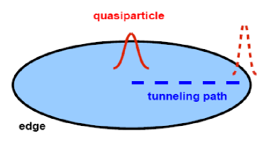
Figure 1: (Color online) Theoretical setup for a disk of a fractional quantum Hall liquid, allowing quasiholes to tunnel through the bulk from the center to the edge.

To study the Moore-Read ground states with and without an $e/4$ or $e/2$ quasihole at a half filling, we start from a three-body interaction $H_{3B}$

$$H_{3B}=-\sum_{i<j<k}S_{ijk}[\nabla^{2}_{i}\nabla^{4}_{j}\delta({\bf r}_{i}-{\bf r}_{j})\delta({\bf r}_{i}-{\bf r}_{k})],$$ (1)

where $S$ is a symmetrizer: $S_{123}[f_{123}]=f_{123}+f_{231}+f_{312}$. The $N$-electron Pfaffian state proposed by Moore and Read moore91 in the lowest Landau level (LLL) representation,

$$\Psi_{\rm MR}(z_{1},z_{2},...,z_{N})=\\ {\rm Pf}\left(1\over{z_{i}-z_{j}}\right)\prod_{i<j}(z_{i}-z_{j})^{2}\exp\left\{-\sum_{i}{|z_{i}|^{2}\over 4}\right\},$$ (2)

is the exact zero-energy ground state of $H_{3B}$ with the smallest total angular momentum $M_{0}=N(2N-3)/2$. In Eq. (2), the Pfaffian is defined by

$${\rm Pf}M_{ij}={1\over 2^{N/2}(N/2)!}\sum_{\sigma\in S_{N}}{\rm sgn}\sigma\prod_{k=1}^{N/2}M_{\sigma(2k-1)\sigma(2k)}$$ (3)

for an $N\times N$ antisymmetric matrix with elements $M_{ij}$.

The three-body interaction also generates a series of zero-energy states with higher total angular momentum, related to edge excitations and bulk quasihole excitations. The $N$-electron Moore-Read ground state with an additional charge $e/4$ quasihole at the origin (so the edge also expand correspondingly due to a fixed number of electrons) has a wavefunction

$$\Psi_{\rm MR}^{e/4}(z_{1},z_{2},...,z_{N})=\\ {\rm Pf}\left({z_{i}+z_{j}}\over{z_{i}-z_{j}}\right)\prod_{i<j}(z_{i}-z_{j})^{2}\exp\left\{-\sum_{i}{|z_{i}|^{2}\over 4}\right\}.$$ (4)

This state is a zero-energy state with total angular momentum $M_{0}+N/2$ in the lowest $2N-1$ orbitals (one more than needed for the Moore-Read state), but not the only one. To generate the unique charge $e/4$ state, we need to introduce a strong repulsive interaction for electrons occupying the lowest two orbitals

$$\Delta H_{e/4}=\lambda c_{1}^{+}c_{1}c_{0}^{+}c_{0},\,\,\,\lambda\rightarrow\infty.$$ (5)

On the other hand, the Moore-Read ground state with a $e/2$ quasihole (i.e., a Laughlin quasihole, equivalent to two $e/4$ quasiholes fused in the identity channel) at the origin,

$$\Psi_{\rm MR}^{e/2}(z_{1},z_{2},...,z_{N})=\left(\prod_{i}z_{i}\right)\Psi_{\rm MR}(z_{1},z_{2},...,z_{N}),$$ (6)

is the unique zero-energy ground state with total angular momentum $M_{0}+N$ in the lowest $2N-1$ orbitals.

The Moore-Read state [Eq. (2)], together with its quasihole states [Eqs. (4) and (6)], can therefore be generated by numerically diagonalizing the three-body Hamiltonian [Eq. (1) with Eq. (5), the artificial repulsion to generate an $e/4$ quasihole] in corresponding finite number of orbitals using the Lanczos algorithm. The wavefunctions can then be supplied to calculate the tunneling amplitudes of the quasiholes. The same numerical procedure can be used to study the tunneling amplitudes for the more realistic situation with a long-range interaction, in which case the variational wavefunctions are no longer eigenstates of the realistic Hamiltonian. For clarity and convenience, we will delay the discussion on how to generate realistic ground state and quasihole states in the presence of long-range interaction (and their comparison with the variational states) to Sec. III.2.

To study the tunneling amplitudes of the quasiholes, let us first consider a single-particle picture, which will help us understand our approach and, later, our results as well. In the disk geometry, the single-particle eigenstates are

$$|m\rangle\equiv\phi_{m}(z)=(2\pi 2^{m}m!)^{-1/2}z^{m}e^{-|z|^{2}/4}.$$ (7)

We assume a single-particle tunneling potential

$$V_{\rm tunnel}(\theta)=V_{t}\delta(\theta),$$ (8)

which breaks the rotational symmetry. Here we calculate the matrix element of $\langle k|V_{\rm tunnel}(\theta)|l\rangle$, related to the tunneling of an electron from state $|l\rangle$ to state $|k\rangle$. One can visualize the tunneling process as a path along the polar angle $\theta=0$ between the two states centered around their maximum amplitude at $|z|=\sqrt{2l}$ and $|z|=\sqrt{2k}$, respectively. One readily obtains

$$v_{p}(k,l)\equiv\langle k|V_{\rm tunnel}(\theta)|l\rangle={V_{t}\over 2\pi}{\Gamma\left({{k+l}\over 2}+1\right)\over\sqrt{k!l!}}.$$ (9)

The interesting limit is that we let $k$ and $l$ tend to infinity, but keep the tunneling distance fixed at $d$, i.e., $|k-l|\sim\sqrt{2k}(d/l_{B})\ll(k+l)$. Alternatively, we can understand $d$ through the angular momentum change $l_{B}^{2}|k-l|/R$, where $R\sim\sqrt{2k}l_{B}$ is the azimuthal size of the single-particle state with momentum $k$ (or $l$ in this limit). We can show (see Appendix A), in this limit,

$$v_{p}(k,l)\sim{V_{t}\over 2\pi}e^{-(k-l)^{2}/4(k+l+2)}\sim{V_{t}\over 2\pi}e^{-d^{2}/(2l_{B})^{2}},$$ (10)

which reflects the overlap of the two Gaussians separated by a distance $d$.

For quasiparticle tunneling at filling fraction $\nu=5/2$, one should, in principle, use wavefunctions in the first excited Landau level (1LL). Evaluating the tunneling matrix element in the 1LL, we obtain an additional prefactor, so

$$v_{p}^{1LL}(k,l)=\left[1-{(k-l)^{2}\over 2(k+l)}\right]v_{p}(k,l).$$ (11)

The sign change in the prefactor at $d\sim l_{B}$ can, unfortunately, cause severe finite-size effect for the numerically accessible range. Nevertheless, in the thermodynamic limit, the prefactor can be approximated by $-(k-l)^{2}/2(k+l)\sim-d^{2}/(2l_{B}^{2})$ and, therefore, the leading decaying behavior is essentially the same. So we will continue to work in the LLL but expect that the leading scaling behavior is the same as in the 1LL.

In the many-body case, we write the tunneling operator as the sum of the single-particle operators,

$${\cal T}=\sum_{i}V_{\rm tunnel}(\theta_{i})=V_{t}\sum_{i}\delta(\theta_{i}).$$ (12)

We are now ready to calculate the tunneling amplitudes $\Gamma^{e/4}=\langle\Psi_{\rm MR}|{\cal T}|\Psi_{\rm MR}^{e/4}\rangle$ and $\Gamma^{e/2}=\langle\Psi_{\rm MR}|{\cal T}|\Psi_{\rm MR}^{e/2}\rangle$ for $e/4$ and $e/2$ quasiholes, respectively. For convenience, we will set $V_{t}=1$ as the unit of the tunneling amplitudes in the following text and figures. As explained in Ref. shopen05, , the matrix elements consist of contributions from the respective Slater-determinant components $|l_{1},...,l_{N}\rangle\in\Psi_{\rm MR}$ and $|k_{1},...,k_{N}\rangle\in\Psi_{\rm MR}^{e/4}$ or $\Psi_{\rm MR}^{e/2}$. Non-zero contributions enters only when $|l_{1},...,l_{N}\rangle$ and $|k_{1},...,k_{N}\rangle$ are identical except for a single pair $\tilde{l}$ and $\tilde{k}$ with angular momentum difference $\tilde{k}-\tilde{l}=N/2$ or $N$ for the quasihole with charge $e/4$ or $e/2$.

For clarity, we also include a pedagogical illustration of the procedure for calculating the tunneling matrix elements in the smallest possible system of four electrons in Appendix B.

III Results

III.1 Short-range interaction

Systems of up to six electrons can be worked out pedagogically using Mathematica as illustrated in Appendix B. For larger systems, we obtain the exact Moore-Read and quasihole wavefunctions by the exact diagonalization of the three-body Hamiltonian [Eq. (1)] using the Lanczos algorithm. The tunneling amplitudes are then evaluated as explained in Sec. II. Figure 2(a) plots the tunneling amplitudes for the $e/4$ and $e/2$ quasiholes in the Moore-Read state as a function of electron number. The result for the $e/4$ quasihole shows a weak increase for $N\leq 10$ followed by a decrease for $N>10$. On the other hand, the result for the $e/2$ quasihole shows a monotonic decrease as the number of electrons increases up to 14. In the largest system, the ratio of the two tunneling matrix elements is slightly less than 20. For comparison, we also plot the tunneling amplitudes $\Gamma^{e/3}$ and $\Gamma^{2e/3}$ for the $e/3$ and $2e/3$ quasiholes in a Laughlin state at $\nu=1/3$ in Fig. 2(b). We also observe a bump in the tunneling amplitude $\Gamma^{e/3}$ for charge $e/3$, followed by a monotonic decrease. We thus expect the $\Gamma^{e/4}$ would eventually also show a monotonic decrease for large enough systems. $\Gamma^{2e/3}$ for charge $2e/3$ shows a much faster decrease, consistent with its larger charge, and thus a larger momentum transfer for the same tunneling distance.

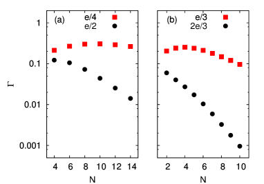
Figure 2: (Color online) tunneling amplitude as a function of number of electrons for (a) $e/4$ and $e/2$ quasiholes in the Moore-Read state at half filling and (b) $e/3$ and $2e/3$ quasiholes in the Laughlin state at $\nu=1/3$.

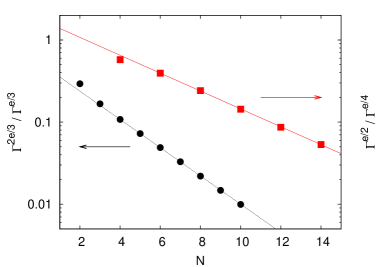
Figure 3: (Color online) The ratio of tunneling matrix elements for $e/2$ quasiholes to $e/4$ quasiholes in the Moore-Read state at half filling, and for $2e/3$ quasiholes to $e/3$ quasiholes in the Laughlin state at $1/3$ filling as a function of number of electrons.

Due to the finite-size bumps in $\Gamma^{e/4}$ and $\Gamma^{e/3}$ for charge $e/4$ and $e/3$, it is difficult to extract the asymptotic behavior in the tunneling amplitudes for these quasiparticles. However, we may expect that such finite-size corrections also exist in the tunneling amplitude for charge $e/2$ and $2e/3$ so we can extract the asymptotic behavior in their ratios. Fortunately, this is indeed the case. We plot $\Gamma^{e/2}/\Gamma^{e/4}$ and $\Gamma^{2e/3}/\Gamma^{e/3}$ in Fig. 3. We find the ratios can be fitted very well by exponentially decaying trends for almost all finite system sizes. The fitting results are

$$\Gamma^{e/2}/\Gamma^{e/4} \simeq 1.78e^{-0.25N},$$ (13)

$$\Gamma^{2e/3}/\Gamma^{e/3} \simeq 0.53e^{-0.40N}.$$ (14)

As will be discussed later, the exponents are related to the charge of the quasiholes and, to a lesser extent, to corrections due to sample geometry, perhaps also to the influence of the neutral component of the charge-e/4 quasiparticles. Quanlitatively, the constant in the exponent of the ratio $\Gamma^{e/2}/\Gamma^{e/4}$ is found to be smaller than that for $\Gamma^{2e/3}/\Gamma^{e/3}$, consistent with the smaller charge and thus smaller charge difference in the half-filled case.

One may question that the tunneling amplitude for a quasihole from the disk center to the disk edge may be different from that for edge to edge, as in the realistic experimental situations. In particular, the former can contain a geometric factor, which can be corrected by mapping the disk to a annulus (or a ribbon) by inserting a large number of quasiholes at the disk center, from which electrons are repelled (see Appendix C for technical details). Inserting $n$ quasiholes to the center of a disk of $N$ electrons in the Moore-Read state, we can write the new wavefunction as

$$\Psi_{\rm MR}^{ne/2}=\left(\prod_{i=1}^{N}z_{i}^{n}\right)\Psi_{\rm MR},$$ (15)

so that each component Slater determinant gets shifted into a new one to be normalized. The first $n$ orbitals from the center are now completely empty and the electrons are occupying orbitals from $n$ to $n+2N-3$. This transformation, of course, also changes the tunneling distance to

$$d(n,N)/l_{B}=\sqrt{2(n+2N-2)}-\sqrt{2n}.$$ (16)

So we can plot data using $d(n,N)$, rather than $n$. Similarly, we can make the same transformation for the Moore-Read state with either an additional charge $e/4$ excitation or an additional charge $e/2$ excitation at the inner edge defined by the inserted $n$ quasiholes. Thus, we can calculate the tunneling amplitudes under the mapping from disk to annulus.

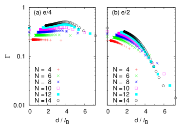
Figure 4: (Color online) (a) The tunneling amplitude $\Gamma^{e/4}$ and (b) the tunneling amplitudes $\Gamma^{e/2}$ as functions of edge-to-edge distance $d(n,N)$. Data is shown up to $n=100$ quasiholes and $N=14$ electrons. The data points at $d=0$ or $n\rightarrow\infty$ limit are exact results as explained in Appendix C.

In Fig. 4, we show the tunneling amplitudes $\Gamma^{e/4}$ and $\Gamma^{e/2}$ for up to $n=100$ quasiholes. We plot them as functions of tunneling distance $d$, which decreases as $n$ increases. It is interesting to note that finite-size effects diminish beyond $d>6l_{B}$ for charge $e/4$ and $d>5l_{B}$ for charge $e/2$. For comparison, we plot the ratio $\Gamma^{e/2}/\Gamma^{e/4}$ as a function of $d$ in Fig. 5. We find that, when we insert more than one quasihole, the ratio of the tunneling amplitudes falls onto a single curve, regardless of the system size $N$ and the number of quasiholes $n$. The curve can be fit roughly to

$${\Gamma^{e/2}(d)\over\Gamma^{e/4}(d)}\sim e^{-0.083(d/l_{B})^{2}}.$$ (17)

We point out that a few points in Fig. 5 can been seen deviated from this behavior. They correspond to the largest $d$ for a given $N$, meaning that there is no quasihole in the bulk, thus corrspond to the bulk-to-edge instead of the edge-to-edge tunneling.

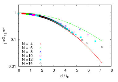
Figure 5: (Color online) The ratio of tunneling amplitudes $\Gamma^{e/2}/\Gamma^{e/4}$ as a function of edge-to-edge distance $d(n,N)$. We also plot Eq. (17) as the solid line to guide the eye. The dashed line is the theoretical estimate based on the charge component only [Eq. (19)].

It is worth pointing out that such behavior is not completely unexpected; in fact, it reflects the asymptotic behavior of the single-particle tunneling matrix and the corresponding charge of the quasiparticles. To see this, we note that for a charge $q$ quasihole to tunnel a distance of $d$, one electron (in each Slater determinant) must hop by a distance of $qd/e$ for the exact momentum transfer. According to the asymptotic behavior in Eq. (10), we expect

$$\Gamma^{q}\sim e^{-(qd/2el_{B})^{2}}.$$ (18)

Therefore, we expect

$${\Gamma^{e/2}\over\Gamma^{e/4}}\sim e^{-[(d/2)^{2}-(d/4)^{2}]/(2l_{B})^{2}}=e^{-0.047(d/l_{B})^{2}},$$ (19)

which we also include in Fig. 5 for comparison.

We thus find that both variational wavefunction calculation and qualitative analysis suggest that the tunneling amplitude of the $e/2$ quasiparticles is smaller than that of the $e/4$ quasiparticles by a Gaussian factor in edge-to-edge distance $d$, which is the main results of this paper. There is, however, a quantitatively discrepancy in the length scale associated with the Gaussian dependence between Eqs. (19) and (17). This indicates that the Gaussian factor in single-electron tunneling matrix element only partially accounts for the Gaussian dependence; the remaining decaying factor thus must be of many-body origin, whose nature is not clear at present and warrants further study.

III.2 Long-range interaction

So far, we have discussed the tunneling amplitudes using the variational wavefunctions, which are exact ground states of the three-body Hamiltonian. These wavefunctions are unique, but in general not the exact ground states of any generic Hamiltonian one may encounter in a realistic sample. In reality, long-range Coulomb interaction is overwhelming, although Landau level mixing can generate effective three-body interaction. bishara09b In this subsection, we explore the quasihole tunneling in the presence of long-range Coulomb interaction. The central questions are the following. First, how can we generate both non-Abelian and Abelian quasiholes in practice? Remember now we do not have the variational Moore-Read state as the exact ground state, so the variational quasihole states are also less meaningful. We attempt to generate and localize quasiholes with a single-body impurity potential; then how close are the corresponding wavefunctions to the variational ones? Second, suppose we have well-defined quasihole wavefunctions, are the results on the tunneling amplitude obtained in the short-range three-body interaction case robust in the presence of long-range Coulomb interaction?

For a smooth interpolation between the short- and long-range cases, we introduce a mixed Hamitonian

$$H_{\lambda}=(1-\lambda)H_{C}+\lambda H_{3B},$$ (20)

as explained in our earlier works. wan06 ; wan08 Here, the dimensionless $\lambda$ interpolates smoothly between the limiting cases of the three-body Hamiltonian $H_{3B}$ ($\lambda=1$) and a two-body Coulomb Hamiltonian $H_{C}$ ($\lambda=0$). $H_{c}$ also includes a background confining potential arising from neutralizing background charge distributed uniformly on a parallel disk of radius $R=\sqrt{4N}$, located at a distance $D$ above the 2DEG. Using the symmetric gauge, we can write down the Hamiltonian for electrons in the 1LL as

$$H_{\rm C}={1\over 2}\sum_{mnl}V_{mn}^{l}c_{m+l}^{\dagger}c_{n}^{\dagger}c_{n+l}c_{m}+\sum_{m}U_{m}c_{m}^{\dagger}c_{m},$$ (21)

where $c_{m}^{\dagger}$ is the electron creation operator for the first excited Landau level (1LL) single electron state with angular momentum $m$. $V_{mn}^{l}$’s are the corresponding matrix elements of Coulomb interaction for the symmetric gauge, and $U_{m}$’s the corresponding matrix elements of the confining potential. We choose $D=0.6$ so the ground state can be well described by the Moore-Read state.

To be experimentally relevant, we also want to generate the quasihole states by a generic impurity potential, rather than by the artificial interaction [Eq. (5)] we used above to generate the unique $e/4$ quasihole state in the three-body case. We consider a Gaussian impurity potential, hu08a

$$H_{imp}(W,s)=W\sum_{m}e^{-m^{2}/2s^{2}}c_{m}^{\dagger}c_{m},$$ (22)

which will trap at the disk center an $e/4$ or $e/2$ quasihole depending on its strength. wan08 Here, $s$ characterizes the range of the potential. Note $H_{imp}=Wc_{0}^{\dagger}c_{0}$ is the short-range limit ($s\rightarrow 0$) of the Gaussian potential in Eq. (22). $W$ is always expressed in units of $e^{2}/(\epsilon l_{B})$.

Earlier studies hu08a ; wan08 have identified $s=2.0$ as a suitable width for the Gaussian trapping potential, which is of roughly the radial size of a quasihole. So we use this value exclusively in the following discussion. One expects that for small $W$, the system remains in the Moore-Read phase without any quasihole excitation in the bulk; for later reference, we use $E_{\lambda}^{0}$ to denote the ground state energy in the momentum subspace of $M=M_{0}=N(2N-3)/2$. As $W$ increases, the impurity potential first tends to attract a charge-$e/4$ quasihole, the smallest charge excitation, at the disk center. This would be reflected in the sudden angular momentum change from $M_{0}$ to $M_{0}+N/2$ of the global ground state, which is also characterized by a depletion of $1/4$ of an electron in the electron occupation number at orbitals with small momentum. We use $E_{\lambda}^{e/4}$ to denote the ground state energy in the subspace of $M=M_{0}+N/2$. When $W$ is increased further, one can trap a charge-$e/2$ quasihole at the center, with ground state having the total angular momentum of $M_{0}+N$; in this momentum subspace, we use $E_{\lambda}^{e/2}$ to denote the ground state energy. We illustrate this scenario for the case for $\lambda=0.5$ in Fig. 6(a), in which we plot the energies of the $e/4$ and $e/2$ quasihole states $E_{\lambda}^{e/4}$ and $E_{\lambda}^{e/2}$, measured from the corresponding $E_{\lambda}^{0}$. More precisely, the $e/4$ quasihole state is energetically favorable for $0.032<W<0.137$. At $W<0.032$, we find $E_{\lambda}^{0}<E_{\lambda}^{e/4}<E_{\lambda}^{e/2}$, while at $W>0.137$, we find $E_{\lambda}^{0}>E_{\lambda}^{e/4}>E_{\lambda}^{e/2}$.

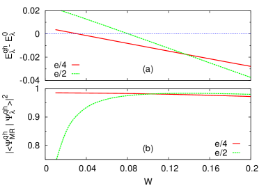
Figure 6: (Color online) (a) Energies of the $e/4$ and $e/2$ quasihole states $E^{qh}_{\lambda}$, measured from the corresponding ground state in the momentum $M_{0}$ subspace $E^{0}_{\lambda}$, as a function of the strength $W$ of the Gaussian trapping potential at the disk center with $s=2.0l_{B}$ for the $\nu=5/2$ state with a mixed Hamiltonian $H_{\lambda}$ ($\lambda=0.5$). The $e/4$ quasihole state is energetically favorable for $0.032<W<0.137$. (b) Overlaps of the $e/4$ and $e/2$ quasihole states $|\Psi_{\lambda}^{qh}\rangle$ for the mixed Hamiltonian with the corresponding variational states $|\Psi_{MR}^{qh}\rangle$ [Eqs. (4) and (6)].

To understand how good these wavefunctions are, we plot, in Fig. 6(b), the overlap of the $e/4$ quasihole state $|\Psi_{\lambda}^{e/4}\rangle$ with the corresponding variational state $|\Psi_{MR}^{e/4}\rangle$ [Eq. (4)], as well as the overlap of the $e/2$ quasihole state $|\Psi_{\lambda}^{e/2}\rangle$ with the corresponding variational state $|\Psi_{MR}^{e/2}\rangle$ [Eq. (6)]. We find that for intermediate $W$ the overlaps are larger than 97%. At small $W$, $|\Psi_{\lambda}^{e/2}\rangle$ does not agree with $|\Psi_{MR}^{e/2}\rangle$ well, but they have very large overlap when the charge-$e/2$ quasihole state energy $E_{\lambda}^{e/2}$ is lower than the correponding energy $E_{\lambda}^{0}$ of the Moore-Read–like state. On the other hand, it is a little surprising to see the excellent agreement between $|\Psi_{\lambda}^{e/4}\rangle$ and $|\Psi_{MR}^{e/4}\rangle$, as they are generated by different Hamiltonian [Eqs. (20) and (1)] with different trapping potential [Eqs. (22) and (5)] respectively. But we note that the smooth Gaussian trapping potential does favor the charge-$e/4$ quasihole state, which has no simultaneous occupation of the lowest two orbitals.

Therefore, we expect that with a moderate mixture of the long-range Coulomb interaction, the results on the tunneling amplitudes are rather robust. In particular, we choose $W=0.1$, at which we have $E_{\lambda}^{0}>E_{\lambda}^{e/2}>E_{\lambda}^{e/4}$ and at which both $|\langle\Psi_{MR}^{e/4}|\Psi_{\lambda}^{e/4}\rangle|^{2}$ and $|\langle\Psi_{MR}^{e/2}|\Psi_{\lambda}^{e/2}\rangle|^{2}$ are very close to 1. For example, we plot the ratio of tunneling amplitudes $\Gamma^{e/2}/\Gamma^{e/4}$ as a function of the number of electrons for $\lambda=0.5$ in Fig. 7. The data points are in good agreement with the trend [Eq. (13)] obtained earlier for the pure three-body case.

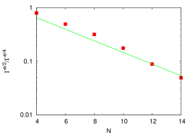
Figure 7: (Color online) The ratio of the tunneling amplitudes for a mixed Hamiltonian as a function of number of electrons. The mix parameter $\lambda=0.5$ and the width and strength of Gaussian potential are $W=0.1$ and $s=2.0$, respectively. The background potential is located at the distance $D=0.6l_{B}$. The dotted line is the exponentially decaying trend line [Eq. (13)] for the pure three-body case as shown in Fig. 3.

So far, we have shown a case where the presence of the long-range interaction has very weak effects on the results of tunneling amplitudes. However, in general, one can expect such an agreement becomes worse as one move farther away from the pure repulsive three-body interaction in the parameter space. To present a more quantitative picture, we plot in Fig. 8 the ratio of tunneling amplitudes $\Gamma^{e/2}/\Gamma^{e/4}$ (without inserting quasiholes at the center, i.e. $n=0$) as a function of $\lambda$ for the 12-electron system with the mixed Hamiltonian $H_{\lambda}$ and a Gaussian trapping potential ($W=2.0$, $s=1.0$). The ratio remains as a constant from $\lambda=1$ down to 0.2, before it fluctuates significantly; the fluctuation is believed to be related to the stripe-like phase near the pure Coulomb case in finite systems, as also revealed in earlier work. wan08 We point out that recent numerical work suggests that the spin-polarized Coulomb ground state at $\nu=5/2$ is adiabatically connected with the Moore-Read wave function for systems on the surface of a sphere, storni09 so the large deviation may well be a finite-size artifact.

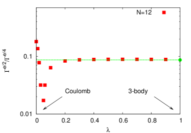
Figure 8: (Color online) The ratio of tunneling amplitudes $\Gamma^{e/2}/\Gamma^{e/4}$ as a function of the mixing parameter between the three-body interaction and Coulomb interaction in a 12-electron system at half-filling in case of $D=0.6l_{B}$. The width and strength of Gaussian potential are $W=0.1$ and $s=2.0$ respectively. The green dot at $\lambda=1$ is the value for the short-range three-body interaction case obtained in Sec. III.1.

Varying parameters, such as $W$, $s$, and $D$, can also lead to larger deviation from the pure three-body case, although we find in generic cases $\Gamma^{e/2}/\Gamma^{e/4}$ remains small. We remind the reader that the Moore-Read phase is extremely fragile. Therefore, we have rather strong constraints on parameters when both the Moore-Read–like ground state and the quasihole states should subsequently be good description of the ground states as the impurity potential strength increases. For example, the window of $D$ for the ground state at $W=0$ to be of Moore-Read nature in the pure Coulomb case is very narrow ($0.51<D/l_{B}<0.76$ for 12 electrons in 22 orbits wan06 ); in this range, the effect of the background potential parameter $D$ on the ratio of tunneling amplitudes is negligible (less than 1% variation). Therefore, we conclude that the small ratio of $\Gamma^{e/2}/\Gamma^{e/4}$ is robust in the presence of the long-range interaction as long as the system remains in the Moore-Read phase.

IV Discussion

In this work we use a simple microscopic model to study quasiparticle tunneling between two fractional quantum Hall edges. We find the tunneling amplitude ratio of quasiparticles with different charges decays with a Gaussian tail as edge-to-edge distance increases. The characteristic length scale associated with this dependence can be partially accounted for by the difference in the charges of the corresponding quasiparticles. More specifically, we find the tunneling amplitude for a charge $e/4$ quasiparticle is significantly larger than a charge $e/2$ quasiparticle in the Moore-Read quantum Hall state, which may describe the observed fractional quantum Hall effect at the filling factor $\nu=5/2$. This result was anticipated in Ref. bishara09, , in which the authors outlined a microscopic calculations that is similar to the discussion in Sec. III.1 (see their Appendix B).

It is worth emphasizing that what we have calculated here are the bare tunneling amplitudes. Under renormalization group (RG) transformations, both amplitudes will grow as one goes to lower energy/temperature, as they are both relevant couplings in the RG sense. The ratio between them, $\Gamma^{e/2}/\Gamma^{e/4}$, will decrease under RG, because $\Gamma^{e/4}$ is more relevant than $\Gamma^{e/2}$, which renders $\Gamma^{e/2}$ even less important than $\Gamma^{e/4}$ at low temperatures. This is clearly consistent with tunneling experiments involving a single point contact,dolevnature ; RaduScience where only signatures of $e/4$ tunneling is seen.

However, the importance of the two kinds of quasiparticles can be reversed in interferometry experiments that look for signatures from interference between two point contacts. This is because the interference signal depends not only on the quasiparticle tunneling amplitudes, but also their coherence lengths when propagating along the edge of fractional quantum Hall samples. Recently, Bishara and Nayak bishara08 found that in a double point-contact interferometer, the oscillating part of the current for charge $q$ quasiparticles can be written as

$$I_{12}^{(q)}\propto\gamma|\Gamma_{1}^{(q)}||\Gamma_{2}^{(q)}|e^{-|x_{12}|/L^{(q)}_{\phi}}\cos\left({{2\pi q\Phi}\over{e\Phi_{0}}}+\delta^{(q)}+\alpha\right),$$ (23)

where $\Gamma_{1,2}^{(q)}$ are the charge $q$ quasiparticle tunneling amplitudes at the two quantum point contacts 1 and 2 with a distance of $x_{12}$. $\gamma$ is a suppression factor resulting from the possible non-Abelian statistics of the quasiparticles. For $q=e/2$, we have $s=1$, while for $q=e/4$, $\gamma=\pm 1/\sqrt{2}$ (or 0) when we have even (or odd) number of $e/4$ quasiparticles in bulk. The sign depends on whether the even number of $e/4$ quasiparticles fuse into the identity channel ($+$) or the fermionic channel ($-$). $\Phi$ is the flux enclosed in the interference loop and $\Phi_{0}=hc/e$ is the magnetic flux quantum. The phase $\delta^{(q)}$ is the statistical phase due to the existence of bulk quasiparticles inside the loop and $\alpha$ the phase $\arg(\Gamma_{1}\Gamma_{2}^{*})$. At a finite temperature $T$, the decoherence length $L^{(q)}_{\phi}$ for the quasiparticle in the Moore-Read state isbishara08

$$L^{(q)}_{\phi}={1\over{2\pi T}}\left({g_{c}^{(q)}\over v_{c}}+{g_{n}^{(q)}\over v_{n}}\right)^{-1},$$ (24)

where $v_{c,n}$ are the charge and neutral edge mode velocities and $g_{c,n}^{(q)}$ the charge and neutral sector scaling exponents for charge $q$ quasiparticles, respectively. Earlier studies by the authors wan06 ; wan08 found that the neutral velocity can be significantly smaller (by a factor of 10) than the charge velocity, leading to a shorter coherence length $L_{\phi}^{(1/4)}$ for charge $e/4$ quasiparticles (less than $1/3$ of $L_{\phi}^{(1/2)}$ for charge $e/2$ quasiparticles in the Moore-Read case, as $L_{\phi}^{(1/2)}$ depends on $v_{c}$ only because it is Abelian and $g_{n}^{(1/2)}=0$). Finite-size numerical analysis hu09 maps out the dependence of $L_{\phi}^{(1/4)}$ and $L_{\phi}^{(1/2)}$ on the strength of confining potential parametrized by $D$ for the Moore-Read state, as summarized in Fig. 9 for $T=25$ mK used in the recent experimental study. willett08 Depending on the size of the interference loop and the strength of the confining potential, the edge transport may exhibit both $e/4$ and $e/2$ quasiparticle interference, $e/2$ quasiparticle interference only, or no quasiparticle interference. In particular, the observation of the $e/4$ quasiparticle interference depends sensitively on the length of the interference loop due to the effect of the confining potential strength on the neutral mode velocity $v_{n}$.

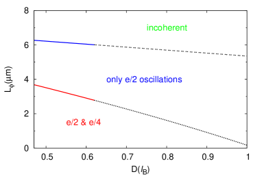
Figure 9: (Color online) Decoherence length $L_{\phi}$ as a function of $D$ for both e/4 (upper line) and e/2 (lower line) quasipaticles in the Moore-Read Pfaffian state. We choose a temperature $T=25$ mK to allow a direct comparison with experiment. willett08 The broken lines above $D=0.62l_{B}$ are obtained by extrapolation, as the Moore-Read–like ground state is no longer stable in a system of 12 electrons in 26 orbitals. We note a stripe phase may emerge below $D=l_{B}$. wan08

We close by stating that by combining the small ratio between $e/4$ and $e/2$ quasiparticle tunneling matrix elements and the fact that $e/2$ quasiparticle has longer coherence length along the edge, it is possible to provide a consistent interpretation of the recent tunnelingdolevnature ; RaduScience and interferencewillett08 ; willett09 experiments. Similar conclusions were reached in a recent comprehensive analysis bishara09 of the interference experiments. willett08 ; willett09 We would like to caution though that a complete quantitative understanding of the experiments is not yet available at this stage due to our incomplete understanding of the actual ground state, mesoscopic effects, and the possible oversimplifications of the microscopic model (for example edge reconstruction wan02 ; yang03 ; overbosch08 may occur and complicate the analysis significantly). Nonetheless, we hope that the quantitative analysis presented here can help solve the puzzle.

Appendix A Single-particle tunneling matrix elements in the large distance limit

In the disk geometry, the single-particle eigenstates are

$$|m\rangle\equiv\phi_{m}(z)=(2\pi 2^{m}m!)^{-1/2}z^{m}e^{-|z|^{2}/4}.$$ (25)

If we assume a single-particle tunneling potential

$$V_{\rm tunnel}=V_{t}\delta(\theta),$$ (26)

the matrix element of $\langle k|V_{t}|l\rangle$, related to the tunneling of an electron from state $|l\rangle$ to state $|k\rangle$, is

$$v_{p}(k,l)\equiv\langle k|V_{\rm tunnel}|l\rangle={V_{t}\over 2\pi}{\Gamma\left({{k+l}\over 2}+1\right)\over\sqrt{k!l!}}.$$ (27)

Using beta functions

$$B(x,y)=\frac{\Gamma\left(x\right)\Gamma\left(y\right)}{\Gamma\left(x+y\right)},$$ (28)

we can rewrite the dimensionless tunneling matrix element as

$$\tilde{v}_{p}(k,l)\equiv\frac{2\pi v_{p}(k,l)}{V_{t}}=\left[\frac{B\left({{k+l}\over 2}+1,{{k+l}\over 2}+1\right)}{B\left(k+1,l+1\right)}\right]^{1/2}.$$ (29)

We are interested in the limit of large $l$ and large $k$, where we can use the asymptotic formula of Stirling’s approximation

$$B(x,y)\sim\sqrt{2\pi}\frac{x^{x-1/2}y^{y-1/2}}{\left(x+y\right)^{x+y-1/2}}$$ (30)

for large $x$ and large $y$. Therefore, we have

$$\tilde{v}_{p}(k,l)\sim\left[\frac{\left(\frac{k+l}{2}+1\right)^{k+l+1}}{\left(k+1\right)^{k+1/2}\left(l+1\right)^{l+1/2}}\right]^{1/2}.$$ (31)

For convenience, we define

$$S=\frac{k+l}{2}\ {\rm and}\ M=\frac{k-l}{2}.$$ (32)

If we further take the limit of $S\gg|M|$, we find

$$\tilde{v}_{p}(k,l) \sim \left(1+\frac{M}{S+1}\right)^{-{{S+M}\over 2}-{1\over 4}}\left(1-\frac{M}{S+1}\right)^{-{{S-M}\over 2}-{1\over 4}}$$ (33)

$$\sim \left[1-\left({M\over{S+1}}\right)^{2}\right]^{-{S\over 2}-{1\over 4}}\left(1-{M\over{S+1}}\right)^{M}$$

$$\sim e^{{M^{2}(S+1/2)\over 2(S+1)^{2}}}e^{-{M^{2}\over{S+1}}}$$

$$\sim e^{-{M^{2}\over 2(S+1)}}.$$

Appendix B Tunneling matrix elements in few-electron systems

In this appendix, we first illustrate the calculation of the tunneling matrix elements in a four-electron system for the Moore-Read state. In this case, the normalized Moore-Read wavefunction can be written as a sum of Slater determinants as

$$\Psi_{\rm MR}={{\sqrt{10}|011110\rangle-\sqrt{2}|101101\rangle+|110011\rangle}\over\sqrt{13}},$$ (34)

where the ket notation denotes a Slater determinant with electrons occuping the single-particle orbitals labeled by 1. For example, $|110011\rangle$ means the normalized antisymmetric wavefunction of four electrons occupying the orbitals with angular momentum 0,1,5,6 (reading from left to right in the ket). This can be obtained by explicitly expanding the Moore-Read state with four electrons (trivial with the help of Mathematica). The corresponding $e/4$ quasihole state, similarly, can be written as

$$\Psi_{\rm MR}^{e/4} = {1\over 5\sqrt{11}}\left(\sqrt{3}|1010101\rangle-4\sqrt{6}|1001110\rangle\right.$$ (35)

$$+ \left.8\sqrt{2}|0110110\rangle-4\sqrt{3}|0111001\rangle\right),$$

and the $e/2$ quasihole state

$$\Psi_{\rm MR}^{e/2} = {1\over 3\sqrt{13}}\left(10|0011110\rangle\right.$$ (36)

$$- \left.2\sqrt{3}|0101101\rangle+\sqrt{5}|0110011\rangle\right).$$

In the many-body case, we write the tunneling operator as the sum of the single-particle operators,

$${\cal T}=V_{t}\sum_{i}\delta(\theta_{i}),$$ (37)

and calculate the tunneling amplitudes $\Gamma^{e/4}=\langle\Psi_{\rm MR}|{\cal T}|\Psi_{\rm MR}^{e/4}\rangle$ and $\Gamma^{e/2}=\langle\Psi_{\rm MR}|{\cal T}|\Psi_{\rm MR}^{e/2}\rangle$ for $e/4$ and $e/2$ quasiholes, respectively. The matrix elements consist of contributions from the respective Slater-determinant components $|l_{1},...,l_{N}\rangle\in\Psi_{\rm MR}$ and $|k_{1},...,k_{N}\rangle\in\Psi_{\rm MR}^{e/4}$ or $\Psi_{\rm MR}^{e/2}$. There are non-zero contributions only when the two sets $\{l_{1},...,l_{N}\}$ and $\{k_{1},...,k_{N}\}$ are identical except for a single pair $\tilde{l}$ and $\tilde{k}$ with angular momentum difference $\tilde{k}-\tilde{l}=N/2$ or $N$ for the quasihole with charge $e/4$ or $e/2$. One should also pay proper attention to fermionic signs.

With some algebra, one obtains, for the four-electron case,

$$\langle\Psi_{\rm MR}|{\cal T}|\Psi_{\rm MR}^{e/4}\rangle = {1\over 5\sqrt{143}}\left[16\sqrt{5}v_{p}(3,5)\right.$$ (38)

$$+ 4\sqrt{30}v_{p}(4,6)+8\sqrt{3}v_{p}(2,4)$$

$$+ \left.8\sqrt{2}v_{p}(0,2)+4\sqrt{6}v_{p}(1,3)\right]$$

and

$$\langle\Psi_{\rm MR}|{\cal T}|\Psi_{\rm MR}^{e/2}\rangle = {1\over 39}\left[10\sqrt{10}v_{p}(1,5)+10\sqrt{2}v_{p}(0,4)\right.$$ (39)

$$+ \left.2\sqrt{30}v_{p}(2,6)\right],$$

where, as before, we define

$$v_{p}(k,l)={V_{t}\over 2\pi}{\Gamma\left({{k+l}\over 2}+1\right)\over\sqrt{k!l!}}.$$ (40)

The numerical values for the two tunneling matrix elements are 0.213 and 0.123, respectively, in units of $V_{t}$. Therefore, in the smallest nontrivial system, we find that the tunneling amplitude for $e/4$ quasiholes is roughly twice as large as that for $e/2$ quasiholes. The example of the four-electron case illustrates how the tunneling amplitudes can be computed. The results are, however, not particularly meaningful as the system size is so small that one cannot really distinguish bulk from edge.

A similar analysis can be performed for a system of six electrons with the help of Mathematica. Due to larger Hilbert space, we will not explicitly write down the decomposition of the ground states and quasihole states by Slater determinants. Instead, we only point out that the tunneling matrix elements are given by

$$\langle\Psi_{\rm MR}|{\cal T}|\Psi_{\rm MR}^{e/4}\rangle=0.267$$ (41)

and

$$\langle\Psi_{\rm MR}|{\cal T}|\Psi_{\rm MR}^{+e/2}\rangle=0.105,$$ (42)

in units of $V_{t}$.

Appendix C Mapping from disk to annulus

Microscopic quantum Hall calculations are commonly based on one of the following geometries (or topologies): torus, sphere, annulus (or cylinder), and disk. In a specific calculation, they are chosen either for convenience, or the need for having different numbers of edge(s). On the other hand one can also map one geometry to another by means of, e.g., quasihole insertion. Here, to connect the theoretical analysis with experiment, we perform a mapping from the disk to the annulus geometry by inserting a large number of quasiholes at the center of the disk, effectively creating an inner edge, as the electron density in the center is suppressed by inserting a small disk of Laughlin quasihole liquid.

After inserting $n$ charge $e/2$ Laughlin quasiholes to the center of an $N$-electron Moore-Read state, the ground state can be written as

$$\Psi_{\rm MR}^{ne/2}=\left(\prod_{i=1}^{N}z_{i}^{n}\right)\Psi_{\rm MR},$$ (43)

where the additional factor transforms each Slater determinant into a new one to be normalized. Let us use the case of four electrons as in Appendix B to illustrate. We note, a Slater determinant $|011110\rangle$ with an addition of $n$ Laughlin quasiholes evolves into another Slater determinant $|(0^{n})011110\rangle$, meaning that the $m$-th (in this example, $m=1$-4) single-particle orbital is now mapped to the $(m+n)$-th orbital. Due to the difference in normalization, the latter determinant should be multiplied by a factor of $F(n;1,2,3,4)$ with a general form of

$$F(n;m_{1},m_{2},\cdots,m_{N})=2^{nN/2}\prod_{i=1}^{N}\sqrt{{(n+m_{i})!\over m_{i}!}}.$$ (44)

Therefore, when we express Eq. (43) explicitly for Eq. (34), we have

$$\Psi_{\rm MR}^{ne/2}={\cal N}\left[F(n;1,2,3,4)\frac{\sqrt{10}}{\sqrt{13}}|(0^{n})011110\rangle\right.\\ -F(n;0,2,3,5)\frac{\sqrt{2}}{\sqrt{13}}|(0^{n})101101\rangle\\ +\left.F(n;0,1,4,5)\frac{1}{\sqrt{13}}|(0^{n})110011\rangle\right],$$ (45)

where ${\cal N}$ is a numerical normalization factor. For $n=1$ we thus obtain exactly Eq. (36) as expected. Interestingly, in the $n\rightarrow\infty$ (ring) limit, the normalized wavefunction becomes, aymptotically,

$$\Psi_{\rm MR}^{ne/2}=C\left[\sqrt{\frac{1}{1!2!3!4!}}\frac{\sqrt{10}}{\sqrt{13}}|(0^{n})011110\rangle\right.\\ -\sqrt{\frac{1}{0!2!3!5!}}\frac{\sqrt{2}}{\sqrt{13}}|(0^{n})101101\rangle\\ +\left.\sqrt{\frac{1}{0!1!4!5!}}\frac{1}{\sqrt{13}}|(0^{n})110011\rangle\right],$$ (46)

where the normalization factor $C$ is, explicitly,

$${1\over C}=\sqrt{\frac{1}{1!2!3!4!}\frac{10}{13}+\frac{1}{0!2!3!5!}\frac{2}{13}+\frac{1}{0!1!4!5!}\frac{1}{13}}.$$ (47)

In the limit of $n\gg N$, we have $v_{p}(n+m_{1},n+m_{2})\rightarrow V_{t}/(2\pi)$. Therefore, the tunneling matrix between the states with $n$ quasiholes and $n+1$ quasiholes becomes

$$\langle\Psi_{\rm MR}^{ne/2}|{\cal T}|\Psi_{\rm MR}^{ne/2+e/2}\rangle\\ =\frac{V_{t}C^{2}}{2\pi}\left[\frac{1}{1!2!3!4!}\frac{10}{13}+\sqrt{\frac{1}{1!2!3!4!}}\frac{\sqrt{10}}{\sqrt{13}}\sqrt{\frac{1}{0!2!3!5!}}\frac{\sqrt{2}}{\sqrt{13}}\right.\\ +\left.\sqrt{\frac{1}{0!2!3!5!}}\frac{\sqrt{2}}{\sqrt{13}}\sqrt{\frac{1}{1!2!3!4!}}\frac{\sqrt{10}}{\sqrt{13}}\right].$$ (48)

The tunneling of $e/4$ quasiholes can be worked out in a similar fashion and we can obtain generically $\left\langle\Psi_{MR}^{ne/2}\mid{\cal T}\mid\Psi_{MR}^{ne/2+e/4}\right\rangle$.

References

- (1) R. L. Willett, J. P. Eisenstein, H. L. Stormer, D. C. Tsui, A. C. Gossard, and J. H. English, Phys. Rev. Lett. 59, 1776 (1987).
- (2) P. L. Gammel, D. J. Bishop, J. P. Eisenstein, J. H. English, A. C. Gossard, R. Ruel, and H. L. Stormer, Phys. Rev. B 38, 10 128 (1988).
- (3) J. P. Eisenstein, R. L. Willett, H. L. Stormer, L. N. Pfeiffer, and K. W. West, Surf. Sci. 229, 31 (1990).
- (4) W. Pan, J.-S. Xia, V. Shvarts, D. E. Adams, H. L. Stormer, D. C. Tsui, L. N. Pfeiffer, K. W. Baldwin, and K. W. West, Phys. Rev. Lett. 83, 3530 (1999).
- (5) W. Pan, H. L. Stormer, D. C. Tsui, L. N. Pfeiffer, K. W. Baldwin, and K. W. West, Solid State Commun. 119, 641 (2001).
- (6) J. P. Eisenstein, K. B. Cooper, L. N. Pfeiffer, and K. W. West, Phys. Rev. Lett. 88, 076801 (2002).
- (7) J. B. Miller, I. P. Radu, D. M. Zumbuhl, E. M. Levenson-Falk, M. A. Kastner, C. M. Marcus, L. N. Pfeiffer, and K. W. West, Nature Phys. 3, 561 (2007).
- (8) H. C. Choi, W. Kang, S. Das Sarma, L. N. Pfeiffer, and K. W. West, Phys. Rev. B 77, 081301(R) (2008).
- (9) W. Pan, J. S. Xia, H. L. Stormer, D. C. Tsui, C. Vicente, E. D. Adams, N. S. Sullivan, L. N. Pfeiffer, K. W. Baldwin, and K. W. West, Phys. Rev. B 77, 075307 (2008).
- (10) C. R. Dean, B. A. Piot, P. Hayden, S. Das Sarma, G. Gervais, L. N. Pfeiffer, and K. W. West, Phys. Rev. Lett. 100, 146803 (2008).
- (11) A. Kitaev, Ann. Phys. 303, 2 (2003).
- (12) J. Preskill, Introduction to Quantum Computation, edited by H.-K. Lo, S. Popescu, and T. P. Spiller (World Scientific, 1998).
- (13) M. H. Freedman, Proc. Natl. Acad. Sci. USA 95, 98 (1998).
- (14) C. Nayak, S. H. Simon, A. Stern, M. Freedman, and S. Das Sarma, Rev. Mod. Phys. 80, 1083 (2008).
- (15) R. H. Morf, Phys. Rev. Lett. 80, 1505 (1998).
- (16) E. H. Rezayi and F. D. M. Haldane, Phys. Rev. Lett. 84, 4685 (2000).
- (17) X. Wan, K. Yang, and E. H. Rezayi, Phys. Rev. Lett. 97, 256804 (2006).
- (18) X. Wan, Z.-X. Hu, E. H. Rezayi, and K. Yang, Phys. Rev. B 77, 165316 (2008).
- (19) M. R. Peterson, Th. Jolicoeur, and S. Das Sarma, Phys. Rev. B 78, 155308 (2008); M. R. Peterson, Th. Jolicoeur, and S. Das Sarma, Phys. Rev. Lett. 101, 016807 (2008).
- (20) G. Möller and S. H. Simon, Phys. Rev. B 77, 075319 (2008).
- (21) A. E. Feiguin, E. H. Rezayi, K. Yang, C. Nayak, and S. Das Sarma, Phys. Rev. B 79, 115322 (2009).
- (22) M. Storni, R. H. Morf, and S. Das Sarma, arXiv:0812.2691.
- (23) G. Moore and N. Read, Nucl. Phys. B 360, 362 (1991).
- (24) S.-S. Lee, S. Ryu, C. Nayak, and M. P. A. Fisher, Phys. Rev. Lett. 99, 236807 (2007).
- (25) M. Levin, B. I. Halperin, and B. Rosenow, Phys. Rev. Lett. 99, 236806 (2007).
- (26) C. Nayak and F. Wilczek, Nucl. Phys. B 479, 529 (1996).
- (27) X. G. Wen, Phys. Rev. B 43, 11025 (1991); Phys. Rev. Lett. 64, 2206 (1990); Phys. Rev. B 44, 5708 (1991).
- (28) C. L. Kane and M. P. A. Fisher, Phys. Rev. B 46, 15233 (1992); K. Moon, H. Yi, C. L. Kane, S. M. Girvin, and M. P. A. Fisher, Phys. Rev. Lett. 71, 4381 (1993); C. L. Kane and M. P. A. Fisher, Phys. Rev. Lett. 72, 724 (1994).
- (29) C. de C. Chamon and X. G. Wen, Phys. Rev. Lett. 70, 2605 (1993).
- (30) P. Fendley, M. P. A. Fisher, and C. Nayak, Phys. Rev. B 75, 045317 (2007).
- (31) A. E. Feiguin, P. Fendley, M. P. A. Fisher, and C. Nayak, Phys. Rev. Lett 101, 236801 (2008).
- (32) S. Das, S. Rao, and D. Sen, Europhys. Lett. 86, 37010 (2009).
- (33) M. Dolev, M. Heiblum, V. Umansky, A. Stern, and D. Mahalu, Nature 452, 829 (2008).
- (34) I. Radu, J. B. Miller, C. M. Marcus, M. A. Kastner, L. N. Pfeiffer, and K. W. West, Science 320, 899 (2008).
- (35) C. de C. Chamon, D. E. Freed, S. A. Kivelson, S. L. Sondhi, and X. G. Wen, Phys. Rev. B 55, 2331 (1997).
- (36) E. Fradkin, C. Nayak, A. Tsvelik, and F. Wilczek, Nucl. Phys. B 516, 704 (1998).
- (37) S. Das Sarma, M. Freedman and C. Nayak, Phys. Rev. Lett. 94, 166802 (2005).
- (38) A. Stern and B. I. Halperin, Phys. Rev. Lett. 96, 016802 (2006).
- (39) P. Bonderson, A. Kitaev, and K. Shtengel, Phys. Rev. Lett. 96, 016803 (2006).
- (40) B. Rosenow, B. I. Halperin, S. H. Simon, and A. Stern, Phys. Rev. Lett. 100, 226803 (2008).
- (41) W. Bishara and C. Nayak, Phys. Rev. B 77, 165302 (2008).
- (42) P. Bonderson, K. Shtengel, and J. K. Slingerland, Phys. Rev. Lett. 97, 016401 (2006).
- (43) L. Fidkowski, arXiv:0704.3291.
- (44) P. Bonderson, K. Shtengel, and J. K. Slingerland, Ann. Phys. 323, 2709 (2008).
- (45) E. Ardonne and E.-A. Kim, J. Stat. Mech. L04001 (2008).
- (46) Y. Ji, Y. Chung, D. Sprinzak, M. Heiblum, D. Mahalu, and H. Shtrikman, Nature 422, 415 (2003).
- (47) Y. Zhang, D. T. McClure, E. M. Levenson-Falk, C. M. Marcus, L. N. Pfeiffer, and K. W. West, Phys. Rev. B 79, 241304(R) (2009).
- (48) F. E. Camino, W. Zhou, and V. J. Goldman, Phys. Rev. B 72, 075342 (2005).
- (49) F. E. Camino, W. Zhou, and V. J. Goldman, Phys. Rev. Lett. 98, 076805 (2007).
- (50) R. L. Willett, L. N. Pfeiffer, and K. W. West, PNAS 106, 8853 (2009).
- (51) R. L. Willett, L. N. Pfeiffer, and K. W. West, unpublished.
- (52) W. Bishara, P. Bonderson, C. Nayak, K. Shtengel, and J. K. Slingerland, Phys. Rev. B 80, 155303 (2009).
- (53) E. Shopen, Y. Gefen, and Y. Meir, Phys. Rev. Lett. 95, 136803 (2005).
- (54) W. Bishara and C. Nayak, arXiv:0906.2516.
- (55) Z.-X. Hu, X. Wan, and P. Schmitteckert, Phys. Rev. B 77, 075331 (2008).
- (56) Z.-X. Hu, E. H. Rezayi, X. Wan, K. Yang, arXiv:0908.3563.
- (57) X. Wan, K. Yang, and E. H. Rezayi, Phys. Rev. Lett. 88, 056802 (2002); X. Wan, E. H. Rezayi, and K. Yang, Phys. Rev. B 68, 125307 (2003).
- (58) K. Yang, Phys. Rev. Lett. 91, 036802 (2003).
- (59) B. J. Overbosch and X.-G. Wen, arXiv:0804.2087.