Discrete Cylindrical Vector Beam Generation from an Array of Optical Fibers

R. Steven Kurti^1,∗, Klaus Halterman¹, Ramesh K. Shori,¹ and Michael J. Wardlaw²

¹Research Division, Physics and Computational Sciences Branch, Naval Air Warfare Center,
China Lake, California, 93555, USA
²Office of Naval Research, Arlington, Virgina, 22203, USA.
^∗Corresponding author: steven.kurti@navy.mil

Abstract

A novel method is presented for the beam shaping of far field intensity distributions of coherently combined fiber arrays. The fibers are arranged uniformly on the perimeter of a circle, and the linearly polarized beams of equal shape are superimposed such that the far field pattern represents an effective radially polarized vector beam, or discrete cylindrical vector (DCV) beam. The DCV beam is produced by three or more beams that each individually have a varying polarization vector. The beams are appropriately distributed in the near field such that the far field intensity distribution has a central null. This result is in contrast to the situation of parallel linearly polarized beams, where the intensity peaks on axis.

OCIS codes:  140.3298, 140.3300, 060.3510.

The propagation of electromagnetic fields from multiple fibers can result in complex far-field intensity profiles that depend crucially on the individual near field polarization and phase. Coherently phased arrays have been used in defense and communications systems for many years, where the antenna ensemble forms a diffraction pattern that can be altered by changing the antenna spacing, amplitude, and relative phase relationships. In the optical regime, similar systems have recently been formed by actively or passively locking the phases of two or more identical optical beams [1, 2, 3, 4]. While coherently combined fiber lasers are increasingly gaining acceptance as sources for high power applications, most approaches involve phasing a rectangular or hexagonal grid of fibers with collimated beams that are linearly polarized along the same axis [5]. The resultant far field diffraction pattern therefore is peaked in the center. If the polarization is allowed to vary, as it does in radial vector beams, the diffraction pattern vanishes in the center[6], which can result in a myriad of device applications, discussed below.

Several types of polarization states have been investigated, including radial and azimuthal [7, 8, 6, 9, 10, 11, 12, 13, 14, 15, 16, 17, 18]. These beams are used in mitigating thermal effects in high power lasers [19, 20, 21], laser machining [22, 23], and particle acceleration interactions [24, 25]. They can even be used to generate longitudinal electric fields when tightly focused [26, 27], and although they are typically formed in free space laser cavities using a conical lens, or axicon, they can also be formed and guided in fibers [28, 29, 30]. Typical methods for creating radially polarized beams fall into two categories: the first involves an intracavity axicon in a laser resonator to generate the laser mode, the second begins with a single beam and rotates the polarization of portions of the beam to create an inhomogeneously (typically radially or azimuthally) polarized beam. In this Letter we demonstrate a novel approach that takes an array of Gaussian beams, each with the appropriately oriented linear polarization, and then superimpose them in the far-field, effectively creating a DCV beam.

Our starting point in determining the propagation of polarized electromagnetic beams is the vector Helmholtz equation, $\nabla\times\nabla\times{\bf E}({\boldsymbol{\rho}},z)-k_{0}^{2}{\bf E}({\boldsymbol{\rho}},z)=0$. We use cylindrical coordinates, so that $\boldsymbol{\rho}$ is the usual transverse coordinate, $k_{0}=\omega/c$, and the usual sinusoidal time dependence has been factored out. Applying Lagrange’s formula permits the wave equation to be written in terms of the vector Laplacian: $\nabla^{2}{\bf E}({\boldsymbol{\rho}},z)+k_{0}^{2}{\bf E}({\boldsymbol{\rho}},z)=0$, which can then be reduced to the paraxial wave equation. The paraxial solutions are then inserted into the familiar Fraunhofer diffraction integral, which for propagation at sufficiently large $z$, yields the electric field,

$${\bf E}(k_{x},k_{y})=\exp\Bigl{(}\frac{ik_{0}\rho^{2}}{2z}\Bigr{)}\frac{\exp(ik_{0}z)}{i\lambda z}$$

$$\times\sum_{j=1}^{N}\int_{0}^{a}rdr\int_{0}^{2\pi}d\phi\,e^{-i{\bf k}\cdot({\bf r}+{\bf s}_{j})}{\bf E}^{0}({\bf r}+{\bf s}_{j},0),$$ (1)

where ${\bf E}^{0}({\bf r}+{\bf s}_{j},0)$ is the incident electric field in the plane of the fiber array.

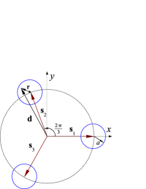
Fig. 1: Example of the multiple fiber setup. A specific case of $N=3$ is shown, where each beam is represented by a circle of radius $a$ and arranged uniformly on a circle of radius $R$. Points within the $i$th hole are located by ${\bf d}={\bf s}_{i}+{\bf r}$, with the vector ${\bf r}$ originating at the center of each hole.

It is clear that longitudinal polarization is not considered here, consistent with the paraxial approximation. The far field intensity will be a complex diffraction pattern that depends on the individual beam intensity profile in the near field as well its polarization state and optical phase. A diagram illustrating the geometry used is shown in Fig. 1, where an array of three circular holes of radius $a$ are equally distributed on the circumference of a circle of radius $R$. The center of each hole is located at ${\bf s}_{j}=R\hat{\bf r}_{j}$, where $\hat{\bf r}_{j}\equiv(\hat{\bf x}\cos\theta_{j}+\hat{\bf y}\sin\theta_{j})$ is the unit radial vector, and ${\bf r}$ is the coordinate relative to each center. The center of each fiber is separated by an angle $\theta_{j}=2\pi(j-1)/N$. One can scale to any number of beams, constrained only by the radius $R$. For identical Gaussian beams, the incident field is expressed as, ${\bf E}^{0}={E}^{0}({\bf r})\hat{\bf r}_{j}$, where ${E}^{0}({\bf r})=E_{0}e^{-r^{2}/w_{0}^{2}}$. This permits Eq. (S0.Ex1) to be separated,

$${\bf E}(k_{x},k_{y})={\cal F}(\rho,z)\sum_{j=1}^{N}e^{-i{\bf k}\cdot{\bf s}_{j}}\hat{\bf r}_{j},$$ (2)

where ${\cal F}(\rho,z)=E_{0}k_{0}/z\int^{a}_{0}rdr\,J_{0}(k_{0}r\rho/z)e^{-r^{2}/w_{0}^{2}}$, and the prefactors that do not contribute to the intensity have been suppressed. It is clear from Eq. (2) that the far field transform preserves the radially symmetric polarization state of the system, as expected. Note that in the limit $w_{0}/a\gg 1$, and using the relation $xJ_{0}(x)=[xJ_{1}(x)]^{\prime}$, we have ${\cal F}(\rho,z)\approx E_{0}(a/\rho)J_{1}(k_{0}a\rho/z)$, which gives the expected Fraunhofer diffraction pattern for a circular aperture of radius $a$. In the opposite limit, where the Gaussian profile is narrow enough so that the aperture geometry has little effect, we have ${\cal F}(\rho,z)\approx E_{0}k_{0}w_{0}^{2}/(2z)\exp[-(k_{0}\rho w_{0}/(2z))^{2}]$. For the multiple beam arrangements investigated, corresponding to $N=3,4,6$, we then can calculate the intensity, $I_{N}$, explicitly:

$${\cal K}_{3}(\phi) =3-\cos({\sqrt{3}}k_{y}R)-2\cos(\frac{\sqrt{3}}{2}k_{y}R)\cos\Bigl{(}\frac{3}{2}k_{x}R\Bigr{)},$$ (3)

$${\cal K}_{4}(\phi) =4\bigl{[}\sin^{2}(k_{x}R)+\sin^{2}(k_{y}R)\bigr{]},$$ (4)

$${\cal K}_{6}(\phi) =4\Bigl{[}\Bigl{(}\cos\Bigl{(}\frac{\sqrt{3}}{2}k_{y}R\Bigr{)}\sin\Bigl{(}\frac{1}{2}k_{x}R\Bigr{)}+\sin\bigl{(}k_{x}R\bigr{)}\Bigr{)}^{2}$$

$$\,\,\,\,\,\,+3\cos^{2}\Bigl{(}\frac{1}{2}k_{x}R\Bigr{)}\sin^{2}\Bigl{(}\frac{\sqrt{3}}{2}k_{y}R\Bigr{)}\Bigr{]},$$ (5)

where $I_{N}\equiv{\cal F}^{2}(\rho,z){\cal K}_{N}(\phi;\rho,z)$, $k_{x}=(k_{0}/z)\rho\cos\phi$ and $k_{y}=(k_{0}/z)\rho\sin\phi$. To rotate the array, one can perform a standard rotation ${\bf r}^{\prime}={\cal R}(\phi^{\prime}){\bf r}$, so e.g., a $\pi/4$ rotation would give, ${\cal K}_{4}(\phi^{\prime})=4(1-\cos(\sqrt{2}k_{x}R)\cos(\sqrt{2}k_{y}R))$.

We employ two different methods to create the DCV beams previously described. In each method, the experimental configuration utilizes collimated Gaussian beams that are in phase. The arrays are cylindrically symmetric both with respect to intensity and polarization. We focus the beams with a transform lens in order to simulate the far field intensity at the lens focus. The focal spot is then imaged onto a camera by a microscope objective in order to fill the CCD array. The laser source is a $100$ mW continuous wave (CW) Nd:YAG operating at $\lambda=1.064\mu$m.

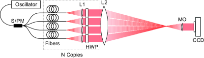
Fig. 2: Diagram of the experimental setup for DCV beam generation. The oscillator output is split and phase modulated (S/PM). The output of each fiber is collimated by means of a lens, L1, and then the polarization is rotated by a half-wave plate (HWP). The beam ensemble is then focused to a point which is imaged by a microscope objective (MO) onto a charge-coupled-device (CCD) array.

The first method (for the case of $N=4$) involves expanding a beam from the Nd:YAG by means of a telescope beam expander to a diameter of about 1cm. The diffractive optical element then creates an $8\times 8$ array of beams. Four of the beams are reflected and made nearly parallel by a segmented mirror, and then linearly polarized upon passing through a set of four half-wave plates. The phases of each beam are made identical by having them pass through articulated glass slides.

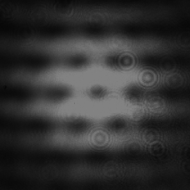
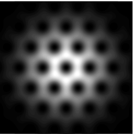
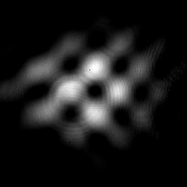
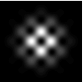
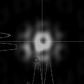
Fig. 3: Far field intensity profiles of effectively radially polarized beams. The left panels correspond to the experimental images and the right panels represent the theoretical results. We consider a 3 (top row), 4 (middle row), and 6 (bottom row) beam arrangement. For $N=3$, we take $w_{0}=32$ $\mu$m and $R=5w_{0}$. For $N=4$, $w_{0}=42$ $\mu$m, and $R=2.7w_{0}$. For $N=6$, we have $w_{0}=43$ $\mu$m and $R=3.8w_{0}$. Note that in general, a radially polarized beam undergoes a discontinuity at the origin, and thus the intensity must vanish there.

The second method (for the case of $N=3$ and $6$), which is simpler for larger arrays, is shown in Fig. 2. In this method the Nd:YAG is coupled into a polarization maintaining fiber. This signal is then split into multiple copies by means of a lithium niobate waveguide 8-way splitter and 8-channel electro-optic modulator. Each path can then have a separate phase modulation to ensure proper phasing of the beams. These signals are then propagated through fiber and coupled out and collimated by a 1 in. lens. The lens is slightly overfilled so the Gaussian outputs of the fibers are truncated at $1.1\times$ (the $e^{-1}$ radius).

Experimental results for the radial vector beam generation found good agreement with theoretical calculations, as illustrated in Fig. 3. Clearly, the interference patterns and symmetry correlate well with the corresponding calculations in the three beam case. In particular, for $N=4$ (middle row), the central null surrounded by a checkerboard peak structure. This pattern differs from the linear polarization by a rotation of $\pi/4$, based on a simple phase argument. The $N=6$ case is shown in the bottom row, where clearly the intensity vanishes at the origin, followed by the formation of bright hexagonal rings. The three beam configuration is shown in the top row, where again there is satisfactory agreement between the calculated and measured results. Any observed discrepancies may be reduced with an appropriately incorporated feedback system. A substantial fraction of the energy in the plots of Fig. 3 is contained within the first regions of high intensity peaks. We illustrate this for the $N=4$ case where the net intensity within a circular region of radius $\rho$, $U(\rho)$, is calculated to be approximately $U(\rho)\approx k_{0}\rho z/(2R)[k_{0}\rho R/z-J_{1}(2k_{0}\rho R/z)]$. Inserting the appropriate parameters and normalizing to the intensity integrated over the entire image plane, yields $50\%$ of the distribution is contained in the neighborhood of the first main peaks.

In conclusion, it has been shown by employing two different configurations, and by carefully controlling the polarization, a central null can be created in the far field. In previous work, the central portion of a phased array of lasers typically has been a peaked function. Now for the first time to our knowledge, a central null has been formed. Similar results have been shown from single aperture lasers using an axicon to generate an annular mode inside a laser cavity. In the present case however, there is direct control over which mode will be generated from the same system. As for scaling, there is no fundamental limitation on the number of beams used. Several methods are available to incorporate a greater number of beams, including concentric beam placement (following the same beam-combining prescription described in this Letter) that could scale in roughly the same pattern as a Bessel beam. It is also possible to use fiber lasers with active phasing, thus potentially scaling to many hundreds of beams[5]. Our system also has a practical advantage over typical high power Gaussian beam applications which have the drawback of having the beam concentrated near the center, where the reflecting beam director (such as a telescope obscuration) resides. Our device on the other hand, has no power propagating along the center axis of the beam, and thus for high power applications requiring a center obscuration telescope beam director, our proposed system offers new advances.

We thank S. Feng for many useful discussions.

References

- [1] “Theory of electronically phased coherent beam combination without a reference beam”, T. M. Shay, Opt. Express 14, 12188 (2006).
- [2] “Self-organized coherence in fiber laser arrays”, H. Bruesselbach, D. C. Jones, M. S. Mangir, M. I. Minden, and J. L. Rogers, Opt. Lett. 30, 1339, (2003).
- [3] “Coherent combining of spectrally broadened fiber lasers,” T. B. Simpson, F. Doft, P. R. Peterson, and A. Gavrielides, Opt. Express 15, 11731 (2007)
- [4] “Coherent addition of fiber lasers by use of a fiber coupler,” Shirakawa, T. Saitou, T. Sekiguchi, and K. Ueda, Opt. Express 10, 1167 (2002).
- [5] “Self-Synchronous and Self-Referenced Coherent Beam Combination for Large Optical Arrays,” T.M. Shay, V. Benham, J.T. Baker, A.D. Sanchez, D. Pilkington, C.A. Lu, IEEE J. Sel. Top. Quant. El. 13, 480 (2007).
- [6] “The formation of laser beams with pure azimuthal or radial polarization,” R. Oron, S. Blit, N. Davidson, A. A. Friesem, Z. Bomzon, and E. Hasman, Appl. Phys. Lett. 77, 3322 (2000).
- [7] “Efficient extracavity generation of radially and azimuthally polarized beams,” G. Machavariani, Y. Lumer, I. Moshe, A. Meir, and S. Jackel, Opt. Lett. 32, 1468 (2007).
- [8] “Intracavity generation of radially polarized CO2 laser beams based on a simple binary dielectric diffraction grating,” T. Moser, J. Balmer, D. Delbeke, P. Muys, S. Verstuyft, and R. Baets, Appl. Opt. 45, 8517 (2006).
- [9] “Simple interferometric technique for generation of a radially polarized light beam,” N. Passilly, R. de Saint Denis, K. A t-Ameur, F. Treussart, R. Hierle, and J. -F. Roch, J. Opt. Soc. Am. A 22, 984 (2005).
- [10] “Generating radially polarized beams interferometrically,” S. C. Tidwell, D. H. Ford, and W. D. Kimura, Appl. Opt. 29, 2234 (1990).
- [11] “Laser beams with axially symmetric polarization,” A V Nesterov et al., J. Phys. D: Appl. Phys. 33 1817 (2000).
- [12] “Generation of a cylindrically symmetric, polarized laser beam with narrow linewidth and fine tunability,” T. Hirayama, Y. Kozawa, T. Nakamura, and S. Sato, Opt. Express 14, 12839 (2006).
- [13] “Radially and azimuthally polarized beams generated by space-variant dielectric subwavelength gratings,” Z. Bomzon, G. Biener, V. Kleiner, and E. Hasman, Opt. Lett. 27, 285 (2002).
- [14] “Generation of a radially polarized laser beam by use of the birefringence of a c-cut Nd:YVO4 crystal,” K. Yonezawa, Y. Kozawa, and S. Sato, Opt. Lett. 31, 2151 (2006).
- [15] “A versatile and stable device allowing the efficient generation of beams with radial, azimuthal or hybrid polarizations,” T. Grosjean, A. Sabac and D. Courjon, Opt. Commun. 252, 12 (2005)
- [16] “Generation of the rotationally symmetric TE01and TM01modes from a wavelength-tunable laser,” J. J. Wynne, IEEE J. Quantum Electron. 10, 125 (1974).
- [17] “Generation of a radially polarized laser beam by use of a conical Brewster prism,” Y. Kozawa and S. Sato, Opt. Lett. 30, 3063 (2005).
- [18] “Fields of a radially polarized Gaussian laser beam beyond the paraxial approximation,” Y. I. Salamin, Opt. Lett. 31, 2619 (2006).
- [19] “2kW, M2 10 radially polarized beams from aberration-compensated rod-based Nd:YAG lasers,” I. Moshe, S. Jackel, A. Meir, Y. Lumer, and E. Leibush, Opt. Lett. 32, 47 (2007).
- [20] “Production of radially or azimuthally polarized beams in solid-state lasers and the elimination of thermally induced birefringence effects,” I. Moshe, S. Jackel, and A. Meir, Opt. Lett. 28, 807 (2003).
- [21] “Generation of radially polarized beams in a Nd:YAG laser with self-adaptive overcompensation of the thermal lens,” M. Roth, E. Wyss, H. Glur, and H.P. Weber Opt. Lett. 30, 1665 (2005).
- [22] “Influence of beam polarization on laser cutting efficency,” V. G. Niziev, A. V. Nestorov, J. Phys. D: Appl. Phys. 32, 1455, (1999).
- [23] “Linear, annular, and radial focusing with axicons and applications to laser machining,” M. Rioux, R. Tremblay, and P.-A. Belanger, Appl. Opt. 17, 1532 (1978).
- [24] “Mono-energetic GeV electrons from ionization in a radially polarized laser beam,” Y. I. Salamin, Opt. Lett. 32, 90 (2007).
- [25] “A tunable doughnut laser beam for cold-atom experiments,” S. M. Iftiquar, J. Opt. B: Quantum Semiclass. Opt. 5, 40 (2003).
- [26] “Focusing of high numerical aperture cylindrical-vector beams,” K. Youngworth and T. Brown, Opt. Express 7, 77 (2000).
- [27] “Sharper focus for a radially polarized beam,” R. Dorn, S. Quabis, and G. Leuches Phys. Rev. Lett. 91, 233901 (2003).
- [28] “An all-fiber device for generating radially and other polarized light beams,” T. Grosjean, D. Courjon and M. Spajer, Opt. Commun. 203, 1 (2002).
- [29] “Generation of cylindrical vector beams with few-mode fibers excited by Laguerre Gaussian beams,” G. Volpe and D. Petrov, Opt. Commun. 237, 89 (2004).
- [30] “Generation of radially polarized mode in Yb fiber laser by using a dual conical prism,” J. Li, K. Ueda, M. Musha, A. Shirakawa, and L. Zhong, Opt. Lett. 31, 2969 (2006).