Quantum dissipative Brownian motion and the Casimir effect

Abstract

We explore an analogy between the thermodynamics of a free dissipative quantum particle and that of an electromagnetic field between two mirrors of finite conductivity. While a free particle isolated from its environment will effectively be in the high-temperature limit for any nonvanishing temperature, a finite coupling to the environment leads to quantum effects ensuring the correct low-temperature behavior. Even then, it is found that under appropriate circumstances the entropy can be a nonmonotonic function of the temperature. Such a scenario with its specific dependence on the ratio of temperature and damping constant also appears for the transverse electric mode in the Casimir effect. The limits of vanishing dissipation for the quantum particle and of infinite conductivity of the mirrors in the Casimir effect both turn out to be noncontinuous.

I Introduction

Recently there has been considerable interest in the study of thermodynamic quantities of a system in the presence of a finite coupling to the heat bath hangg06 ; hoerh08 ; bandy08 ; wang08 ; hangg08 ; kumar09 ; ingol09 ; bandy09 . In contrast to the classical equilibrium state, the stationary quantum state depends on the system-bath coupling and thus the low-temperature regime is of particular interest. Even on a conceptual level, for finite system-bath coupling, the correct definition of basic thermodynamic quantities like the specific heat has proven to be far from obvious hangg06 ; hangg08 .

The thermodynamics of a free particle coupled to a heat bath is particularly rich. In the absence of an environment, the free particle behaves classically for any nonvanishing temperature. This unusual behavior is a consequence of the lack of any energy scale besides the thermal energy $k_{B}T=1/\beta$ where $T$ is the temperature and $k_{B}$ is the Boltzmann constant. The situation changes once the particle is confined to a finite region in space of length $L$ or coupled to an environment. In the first case, an energy scale $\hbar^{2}/2ML^{2}$ appears where $M$ is the mass of the particle, while in the latter case, the relaxation frequency $\gamma$ due to the coupling to the environment yields an energy scale $\hbar\gamma$.

It is the second scenario which one is interested in when studying the effect of a finite coupling to the heat bath. Then all thermodynamic quantities will depend on the dimensionless temperature $k_{B}T/\hbar\gamma$. As a first example of the intricacy associated with the limit of vanishing damping, $\gamma\to 0$, in such a situation, we mention the diffusion of a free Brownian particle. The long-time behavior is governed by the diffusion constant $D=k_{B}T/M\gamma$. For any nonvanishing value of $\gamma$, one finds diffusive motion while for $\gamma=0$, the motion will be ballistic. The limit $\gamma\to 0$ will thus be qualitatively different from $\gamma=0$.

The peculiar combination $k_{B}T/\hbar\gamma$ implies that for any nonzero temperature, the free particle will be driven into the classical regime when $\gamma$ approaches zero. On the other hand, for any nonzero value of $\gamma$, there exists a low-temperature region which is essentially quantum in nature and depends on the coupling to the heat bath hangg06 ; hangg08 . In this regime, the specific heat approaches zero as temperature goes to zero while the specific heat of an isolated free particle remains at its classical value $k_{B}/2$.

Interestingly, for appropriately chosen coupling between the free particle and the heat bath, the entropy exhibits a nonmonotonic behavior as a function of temperature. Evaluation of the specific heat according to standard thermodynamic relations results in negative values. However, as entropy and specific heat pertain only to a subsystem formed by the free particle, this is not in contradiction to basic thermodynamic stability criteria ingol09 .

While the free particle might appear to be rather special, we will argue in the present paper that the scenario just discussed also applies in the context of the Casimir effect (for a review see borda01 ; milto04 ; njp06 ; lambr06 and references therein). There, in the simplest case, one considers the force between two parallel plane mirrors separated by a distance $L$ due to the boundary conditions imposed by the mirrors on the electromagnetic field casim48 . The coupling between the electrons in the mirrors and the electromagnetic field therefore is essential, in particular if real mirrors are considered. On the one hand, the reflectivity of metals goes to zero for high frequencies on a scale determined by the plasma frequency $\omega_{P}$. On the other hand, as long as normal metals are considered, the dc conductivity $\sigma_{0}$ is finite. Within the Drude model this finite conductivity unavoidably comes with a relaxation frequency $\gamma$.

The conductivity of metals like gold employed in measurements of the Casimir force is so large that the relaxation frequency $\gamma$ is much smaller than the plasma frequency $\omega_{P}$ and smaller than the frequency $c/L$ associated with mirror separations between 20 nm and $6\,\mu\text{m}$ used in experiments so far decca07 ; munda07 ; chan08 ; vanzw08 ; munda09 ; jourd09 ; masud09 ; deman09 . On the other hand, at room temperature the energy scales $k_{B}T$ and $\hbar\gamma$ are comparable, thus opening the opportunity to explore the transition from the classical to the quantum regime.

As we will show in this paper, if apart from the thermal scale the relaxation frequency $\gamma$ represents the smallest frequency scale, essential low-temperature features of the Casimir effect within the Drude model are analogous to those pointed out above for the free Brownian particle. In our opinion, this analogy will be valuable for the understanding of the thermal Casimir effect and shed additional light on thermodynamic peculiarities related to the transverse electric mode klimc06 ; brevi06 ; milto08 ; torge04 like the negative entropy found for the Drude model.

We will start in Sec. II by reviewing recent results on the thermodynamics of the free Brownian particle and presenting new results on the entropy which is of particular interest in relation to the Casimir effect. In Sec. III, essential properties of a Drude metal like its permittivity and reflectivity are introduced. Sec. IV is devoted to the thermal corrections to the zero-temperature Casimir force. The low-temperature behavior of the Casimir force is discussed and the leading thermal correction for the transverse electric mode within the Drude model is obtained on the basis of a scattering approach. In addition, the leading thermal correction for the transverse magnetic mode is presented. In Sec. V, we establish the analogy between the free Brownian particle and the thermal corrections to the Casimir force due to the transverse electric mode within the Drude model. This analogy will be further discussed in Sec. VI in terms of the free energy and the entropy. Finally, in Sec. VII we present our conclusions. Technical details concerning the derivation of the leading thermal corrections to the Casimir force within the Drude model will be given in an appendix.

II Thermodynamics of the free Brownian particle

As a paradigm for the peculiar effects of a finite system-bath coupling on the thermodynamics of the system degree of freedom, we consider a free particle of mass $M$. For normalization purposes, the particle will be confined to a region of size $L$ which is assumed to be sufficiently large so that the energy quantization is irrelevant for the temperatures of interest, i.e. $\hbar^{2}\beta/2mL^{2}\ll 1$. Even for microscopic systems like a hydrogen atom and the lowest temperatures attainable today, choosing $L=1\,\text{cm}$ would easily meet this condition.

The free particle is assumed to be bilinearly coupled to a bath of harmonic oscillators. The total Hamiltonian can then be cast into the form

$$H=H_{S}+H_{B}+H_{SB}$$ (1)

with the system Hamiltonian

$$H_{S}=\frac{P^{2}}{2M}$$ (2)

where $P$ is the momentum of the particle, the bath Hamiltonian describing an infinite collection of harmonic oscillators of masses $m_{n}$ and frequencies $\omega_{n}$,

$$H_{B}=\sum_{n=1}^{\infty}\frac{p_{n}^{2}}{2m_{n}}+\frac{m_{n}}{2}\omega_{n}^{2}x_{n}^{2}\,,$$ (3)

and the Hamiltonian

$$H_{SB}=\sum_{n=1}^{\infty}-m_{n}\omega_{n}^{2}x_{n}Q+\frac{m_{n}\omega_{n}^{2}}{2}Q^{2}$$ (4)

coupling the free particle and the bath oscillators via their respective positions $Q$ and $x_{n}$. For a more detailed discussion of this Hamiltonian, we refer the reader to the literature dittr98 ; weiss99 ; ingol02 . It is worth noting that the second term appearing in (4) is crucial to ensure the translational invariance of the free Brownian particle. Furthermore, the bath parameters $m_{n}$ and $\omega_{n}$ are sufficient to model any linear heat bath grabe88 .

As a starting point for the following thermodynamic considerations, we introduce the reduced partition function hangg06 ; grabe88 ; calde83 ; grabe84 ; ford85

$$\mathcal{Z}=\frac{\text{Tr}_{S+B}[\exp(-\beta H)]}{\text{Tr}_{B}[\exp(-\beta H_{B}]}\,.$$ (5)

In the absence of any coupling between system and bath, this quantity reduces to the partition function of the system while otherwise it accounts for the influence of the coupling. Any quantity which can be obtained by a linear operation from the logarithm of this partition function can be viewed as a difference of the quantities related to the system and bath on one hand and to the bath alone on the other hand ingol09 . It thus describes the effect induced by coupling a system degree of freedom to the heat bath. Such quantities therefore do not need to satisfy thermodynamic conditions which have to be imposed on closed systems.

For a free Brownian particle, the reduced partition function defined in (5) is given by hangg08

$$\mathcal{Z}=\frac{L}{\hbar}\left(\frac{2\pi m}{\beta}\right)^{1/2}\prod_{n=1}^{\infty}\frac{\xi_{n}}{\xi_{n}+\hat{\gamma}(\xi_{n})}\,.$$ (6)

Here,

$$\xi_{n}=\frac{2\pi n}{\hbar\beta}$$ (7)

are the Matsubara frequencies and $\hat{\gamma}$ is the Laplace transform of the damping kernel which for ohmic damping is simply given by a constant, i.e. $\hat{\gamma}(\xi)=\gamma$. In order to ensure the convergence of the infinite product, a high-frequency cutoff has to be introduced which is often chosen to be of the form footnote1

$$\hat{\gamma}(\xi)=\frac{\gamma\omega_{c}}{\xi+\omega_{c}}\,.$$ (8)

In the internal energy and therefore also the free energy, a finite cutoff $\omega_{c}$ is needed while the limit of infinite cutoff can be taken for the entropy, for example. As we will see at the end of this section, it may however be interesting to keep $\omega_{c}$ finite and even to consider the case of very small cutoff frequencies.

Based on (6), we define an entropy $S$ by means of the standard thermodynamic relation

$$\frac{S}{k_{B}}=\frac{\partial}{\partial T}[k_{B}T\log(\mathcal{Z})]\,.$$ (9)

We will carry out the discussion of the entropy in two steps which both lead to results of relevance for our later considerations of the Casimir effect. First, we will restrict ourselves to the limit of infinite cutoff frequency $\omega_{c}$ and then, in a second step, we admit finite cutoff frequencies.

From (9) one finds with (6) and (8) in the limit of $\omega_{c}\to\infty$ the entropy

$$\frac{S}{k_{B}} =\frac{S_{0}}{k_{B}}+\log\left[\Gamma\left(1+\frac{\hbar\beta\gamma}{2\pi}\right)\right]-\frac{\hbar\beta\gamma}{2\pi}\psi\left(\frac{\hbar\beta\gamma}{2\pi}\right)$$ (10)

$$\quad-\frac{1}{2}\log(\hbar\beta\gamma)+\frac{\hbar\beta\gamma}{2\pi}-\frac{1}{2}\,,$$

where $\Gamma(x)$ is the gamma function and $\psi(x)$ its logarithmic derivative. In the zero-temperature limit, the entropy takes the value

$$\frac{S_{0}}{k_{B}}=\frac{1}{2}\log\left[2\pi\frac{ML^{2}\gamma}{\hbar}\right]$$ (11)

which depends logarithmically on the box size $L$. The existence of this non-vanishing entropy $S_{0}$ is a consequence of the fact that we do not account for the level spacing due to the finite box size as discussed at the beginning of this section. We rather are interested in the influence of a finite damping strength. In the following, we will concentrate on the difference $S-S_{0}$ which is independent of $L$.

For high temperatures, one finds from (10)

$$\frac{S-S_{0}}{k_{B}}=\frac{1}{2}\left[\log\left(\frac{k_{B}T}{\hbar\gamma}\right)+1\right]\,.$$ (12)

In view of the entropy constant (11) it follows that the high-temperature behavior of the entropy $S$ does not depend on the damping strength $\gamma$. This reflects the fact that equilibrium properties in classical thermodynamics do not depend on the strength of the coupling between system and heat bath. At the same time, the high-temperature expression for the entropy represents the entropy of an undamped free particle for arbitrary temperatures $T>0$. By means of the relation

$$C=T\frac{\partial S}{\partial T}$$ (13)

between specific heat $C$ and entropy $S$, the logarithmic dependence of the entropy on the inverse temperature leads to a constant specific heat $C=k_{B}/2$ for any nonvanishing temperature in the absence of damping.

In the presence of damping, quantum effects arise in the low-temperature regime where (10) yields

$$\frac{S-S_{0}}{k_{B}}=\frac{\pi}{3}\frac{k_{B}T}{\hbar\gamma}\,.$$ (14)

This expression diverges for vanishing damping constant, clearly indicating that the limit $\gamma\to 0$ is nontrivial at low temperatures. In contrast to the constant specific heat found for the undamped particle, the specific heat now depends linearly on temperature.

The temperature dependence of the difference between the entropy (10) and its zero-temperature value (11) is depicted in Fig. 1 as solid line together with the high- and low-temperature expressions (12) and (14), respectively, as dotted lines.

Figure 1: Temperature dependence of the difference between the entropy (10) and its zero-temperature value (11) for a free Brownian particle subject to ohmic dissipation of strength $\gamma$. The dotted lines correspond to the high- and low-temperature expressions (12) and (14), respectively.

From (10) it is clear, that the difference $S-S_{0}$ depends on the temperature only through the dimensionless quantity $\hbar\beta\gamma$ which, in view of our discussion in the introduction, should be expected. As $\gamma$ decreases, the high-temperature region effectively becomes increasingly larger. However, the divergence of (12) in the zero-temperature limit is avoided by a crossover to the low-temperature behavior (14) below temperatures of the order of $\hbar\gamma/k_{B}$. In this low-temperature regime, the dependence on $\hbar\beta\gamma$ immediately implies a nontrivial limit of vanishing coupling to the heat bath as discussed in connection with (14).

As we will see in more detail in the discussion of the Casimir entropy, a difference between the Casimir problem and the free Brownian particle consists in the value taken by the entropy at zero temperature. While the Casimir entropy goes to zero in that limit, we found a nonvanishing entropy constant $S_{0}$ for the free Brownian particle. $S_{0}$ will be positive provided that the broadening of the levels due to the coupling to the heat bath is larger than the ground-state energy. The Casimir entropy, on the other hand, can exhibit negative values of the entropy under certain circumstances. This raises the question whether in the case of the free Brownian particle the entropy can drop below $S_{0}$. While this does not necessarily imply a negative entropy, the entropies in the two situations would nevertheless behave nonmontonically. As a direct consequence, measurable thermodynamic quantities like the specific heat could in both cases take on negative values. This was indeed found for the free Brownian particle hangg08 .

For strictly ohmic damping, $\hat{\gamma}(\xi)=\gamma$, the entropy $S$ will always be larger than $S_{0}$ and we therefore have to consider the case of finite cutoff frequency $\omega_{c}$. If $\hat{\gamma}^{\prime}(0)<-1$, which for the damping kernel (8) corresponds to $\omega_{c}<\gamma$, there exists a temperature range where $S-S_{0}<0$ and where the specific heat becomes negative hangg08 . The nonmonotonic behavior of the entropy is shown in Fig. 2 for decreasing values of the cutoff frequency $\omega_{c}/\gamma=\infty,1,0.1,$ and $0.01$ from the upper to the lower curve. In addition to the appearance of a nonmonotonic behavior, one observes that with decreasing cutoff frequency $\omega_{c}$ and therefore decreasing coupling to the bath oscillators, the entropy follows the high-temperature behavior (12) represented by the dotted line down to lower temperatures. This underlines once more the nontrivial limit of vanishing coupling to the heat bath.

Figure 2: Temperature dependence of the difference between the entropy (10) and its zero-temperature value (11) for a free Brownian particle subject to ohmic dissipation with a high-frequency cutoff $\omega_{c}/\gamma=\infty,1,0.1$, and $0.01$ from the upper to the lower curve. The dotted line represents the high-temperature expression (12).

The nonmonotonicity of the entropy however does not put the thermodynamic stability of the system in question. As pointed out before, an entropy based on the reduced partition function (5) is the difference of two positive entropies referring to the heat bath and the heat bath in the presence of the free particle ingol09 .

III Plasma and Drude models

In the context of this paper, we are not interested in a realistic description of experiments decca07 ; munda07 ; chan08 ; vanzw08 ; munda09 ; jourd09 ; masud09 ; deman09 . exploring the Casimir effect but rather in a theoretical analysis of the effects of a finite conductivity of the mirrors, in particular at low temperatures. We therefore assume an idealized geometrical setup where two infinitely large metallic plane mirrors are positioned in parallel at a distance $L$ of each other. By an appropriate choice of the permittivity, we will account for basic features of the optical response of real mirrors, namely the low reflectivity at high frequencies and the finite conductivity at low frequencies.

The high-frequency optical response of a metal is well described within the plasma model in terms of the relative permittivity

$$\varepsilon(\omega)=1-\frac{\omega_{P}^{2}}{\omega^{2}}\,.$$ (15)

Here, $\omega_{P}$ denotes the plasma frequency which is related to the plasma wavelength by

$$\lambda_{P}=\frac{2\pi c}{\omega_{P}}$$ (16)

where $c$ is the speed of light. For gold, the plasma wavelength is $0.136\,\mu$m and the finite plasma frequency becomes appreciable for mirror distances $L\lesssim 1\,\mu$m genet00 . In the following, we assume for all numerical calculations a fixed value of $\lambda_{P}/L=0.136$, corresponding to a mirror distance of one micrometer which is a typical order of magnitude in experiments.

The relative permittivity $\varepsilon(\omega)$ is related to the conductivity $\sigma(\omega)$ of the mirrors by

$$\varepsilon(\omega)=1+i\frac{\sigma(\omega)}{\omega}\,.$$ (17)

Here, the conductivity $\sigma$ is expressed as a frequency from which the conductivity in SI units is obtained as $\varepsilon_{0}\sigma$ with the permittivity of vacuum $\varepsilon_{0}$. According to (17), applying the relative permittivity (15) for all frequencies down to $\omega=0$ would imply the assumption of an infinite dc conductivity which is certainly unacceptable for normal metals.

The simplest model ensuring a finite dc conductivity is the Drude model with the relative permittivity

$$\varepsilon(\omega)=1-\frac{\omega_{P}^{2}}{\omega(\omega+i\gamma)}\,.$$ (18)

It is obtained from (15) by introducing a relaxation frequency $\gamma$ and leads to the dc conductivity

$$\sigma_{0}=\frac{\omega_{P}^{2}}{\gamma}\,.$$ (19)

We will assume $\gamma$ to be independent of temperature thus implying a nonvanishing conductivity at zero temperature due to crystal defects or impurities tto0 .

Taking the dc conductivity of gold, $\varepsilon_{0}\sigma_{\text{Au}}=4.52\cdot 10^{7}\,(\Omega\text{m})^{-1}$, one obtains for the relaxation frequency $\gamma\approx 2.7\cdot 10^{-3}\omega_{P}$. Assuming mirror distances of one micrometer or smaller, we find $\gamma L/c\lesssim 0.125$. The relaxation frequency therefore is typically small compared to $\omega_{p}$ and to $L/c$. On the other hand, for the conductivity assumed here, the ratio $\hbar\gamma/k_{B}T$ is of the order of one at room temperature.

Although the Drude model cannot be expected to give an accurate description of all details of the permittivity of a real metal lambr00 ; sveto08 , it is the simplest model accounting for a finite dc conductivity and therefore deserves to be analyzed in detail. As apart from the thermal frequency $k_{B}T/\hbar$ the relaxation frequency $\gamma$ is the smallest frequency scale in the problem, it is interesting to investigate the limit $\gamma\to 0$.

The reason why this limit can be nontrivial becomes apparent when the reflection coefficients are considered. Before doing so, we introduce the notation for frequencies and wavevectors which will be used in the sequel. The wavevector of an electromagnetic mode is $\mathbf{k}=(\mathbf{k}_{\parallel},k_{\bot})$ where $k_{\bot}$ denotes the component orthogonal to the mirrors while $\mathbf{k}_{\parallel}$ is a two-dimensional vector parallel to the mirrors. Although it is possible and sometimes useful to keep frequencies real sveto07 ; ellin08 , here we will employ imaginary frequencies $\xi=-i\omega$ and wave-vector components $\kappa=-ik_{\bot}$ so that the dispersion relation becomes $\xi^{2}=c^{2}(\kappa^{2}-\mathbf{k}_{\parallel}^{2})$.

With this notation the reflection coefficient for the transverse electric (TE) mode is obtained as

$$r_{\text{TE}}(i\xi,i\kappa)=\frac{\sqrt{c^{2}\kappa^{2}+[\varepsilon(i\xi)-1]\xi^{2}}-c\kappa}{\sqrt{c^{2}\kappa^{2}+[\varepsilon(i\xi)-1]\xi^{2}}+c\kappa}$$ (20)

while for the transverse magnetic (TM) mode one finds

$$r_{\text{TM}}(i\xi,i\kappa)=\frac{\sqrt{c^{2}\kappa^{2}+[\varepsilon(i\xi)-1]\xi^{2}}-\varepsilon(i\xi)c\kappa}{\sqrt{c^{2}\kappa^{2}+[\varepsilon(i\xi)-1]\xi^{2}}+\varepsilon(i\xi)c\kappa}\,.$$ (21)

An important difference between the plasma model and the Drude model with direct implications for the reflection coefficients is the fact that the limit of $\xi^{2}[\varepsilon(i\xi)-1]$ for $\xi\to 0$ tends to $\omega_{P}^{2}$ for the plasma model while it vanishes for the Drude model. This does not affect the zero frequency reflection of the TM mode but for the TE mode one finds a vanishing reflection coefficient $r_{\text{TE}}(0,i\kappa)$ for the Drude model in contrast to a nonvanishing value for the plasma model bostr00 .

Clearly, such a behavior is not compatible with a continuous transition from the Drude to the plasma model for $\gamma\to 0$. The zero-frequency behavior of the reflection coefficient has a dramatic consequence for the Casimir force at high temperatures. While within the plasma model the TE modes contribute to the Casimir force, this is not the case within the Drude model. As a consequence, in the latter case the Casimir force arises only from the TM modes and is thus reduced by a factor of two with respect to the plasma model bostr00 . Recent years have seen an extensive debate about the existence of this reduction factor and its compatibility with thermodynamics (for a review see e.g. Refs. klimc06, and milto08, ). Interestingly, a rather independent approach based on a microscopic study of the force between two slabs containing an electron plasma in the classical and semiclassical regime also led to a reduction of the Casimir force by a factor of two janco05 ; buenz05a as does the consideration of the classical Bohr-van Leeuwen theorem bimon09 .

In the following, we will analyze in detail the transition from the Drude to the plasma model. Of particular interest will be the case of low temperatures. This limit is of relevance for the leading thermal corrections to the Casimir force and also in the context of the ongoing debate about a possible violation of the third law of thermodynamics klimc06 ; milto08 . In the course of the discussion it will become clear that the transition from the Drude to the plasma model for the TE mode bears close analogy to the transition from a free Brownian particle to a free particle hangg06 ; hangg08 ; ingol09 .

IV Thermal corrections to the Casimir force

For the case of only partially reflecting mirrors, the radiation pressure of the electromagnetic field modes on the mirrors can be obtained from a scattering formalism jaeke91 . Performing the integration over the modes in imaginary frequency $\xi$ and imaginary orthogonal component $\kappa$ of the wavevector, one finds for the Casimir force between two parallel mirrors genet03

$$F=\frac{\hbar A}{\pi^{2}}\sum_{n=0}^{\infty}{}^{\prime}\int_{0}^{\infty}d\xi\cos(n\hbar\beta\xi)\mathbb{F}(\xi)\,.$$ (22)

Here, $A$ is the surface of the mirror, the prime at the sum sign indicates that the $n=0$ term contributes only with a factor one-half, and

$$\mathbb{F}(\xi)=\int_{\xi/c}^{\infty}d\kappa\,\kappa^{2}f(i\xi,i\kappa)\,.$$ (23)

In the integrand ,

$$f(i\xi,i\kappa)=\sum_{p=\mathrm{TE,TM}}f_{p}(i\xi,i\kappa)$$ (24)

is the closed-loop function where one has to sum over the two polarizations $p$ with

$$f_{p}(i\xi,i\kappa)=\frac{r_{p}^{2}(i\xi,i\kappa)}{\exp(2\kappa L)-r_{p}^{2}(i\xi,i\kappa)}\,.$$ (25)

In this expression, we have assumed for simplicity that the two mirrors have the same reflection properties.

The $n=0$ term in (22) corresponds to the zero-temperature Casimir force arising from the vacuum fluctuations of the electromagnetic field between the mirrors. All terms with $n>0$ describe thermal corrections due to real photons present at finite temperatures. Equation (22) is therefore particularly well suited to separate off the zero-temperature force and to determine the low-temperature behavior.

If the conditions of validity of the Poisson formula are met milto04 ; reyna04 , we recover from (22) the Lifshitz formula of the Casimir force lifsh56

$$F=\frac{A}{\pi\beta}\sum_{n=0}^{\infty}{}^{\prime}\mathbb{F}(\xi_{n})\,,$$ (26)

where $\mathbb{F}(\xi)$ has been defined in (23) and $\xi_{n}$ are the Matsubara frequencies (7). Here, the $n=0$ term allows to immediately read off the dominant contribution to the force at high temperatures. For the TE mode within the Drude model, the reflection coefficient and therefore the closed-loop function vanish at $\xi=0$. According to (26), the TE modes thus do not contribute to the high-temperature behavior, resulting in the reduction of the force by a factor of two mentioned above bostr00 . The expression (26) is not restricted to high temperatures though and a corresponding expression has recently been employed to analyze the low-temperature behavior of the free energy hoye07 ; brevi08 ; ellin08a .

For the discussion of the thermal corrections it is convenient to introduce a dimensionless factor by dividing the Casimir force $F$ through the Casimir force for ideal mirrors at zero temperature

$$F_{\text{Cas}}=\frac{\hbar cA\pi^{2}}{240L^{4}}\,.$$ (27)

This expression accounts for both the TE and the TM mode and will be used even in cases where only one of the modes is considered. We thus define the factor

$$\eta_{F}=\frac{F}{F_{\text{Cas}}}=\eta_{F}^{0}+\eta_{F}^{T}$$ (28)

where $\eta_{F}^{0}$ is the zero-temperature contribution arising from the $n=0$ term in (22) and

$$\eta_{F}^{T}=\frac{240L^{4}}{c\pi^{4}}\sum_{n=1}^{\infty}\int_{0}^{\infty}d\xi\cos(n\hbar\beta\xi)\mathbb{F}(\xi)$$ (29)

describes the thermal corrections.

Before entering into a detailed analysis of the TE mode in Sec. V, we discuss the temperature dependence of the Casimir force for the TE and TM modes in the plasma model and the Drude model. Figure 3 displays the thermal contribution $\eta_{F}^{T}$ defined in (29) as a function of the dimensionless temperature $k_{B}TL/\hbar c$ for $\lambda_{P}/L=0.136$ and the dc conductivity of gold $\sigma_{\text{Au}}$. The solid lines represent results based on the Lifshitz formula (26) while the filled and open symbols represent data obtained by evaluating (22) for the TE and the TM mode, respectively. As Fig. 3 indicates, the two approaches (22) and (26) lead indeed to the same results, confirming that the Poisson resummation can also be employed for the Drude model. For the numerical evaluation of the force, the expression (22) works well at low temperatures while (26) is advantageous at higher temperatures.

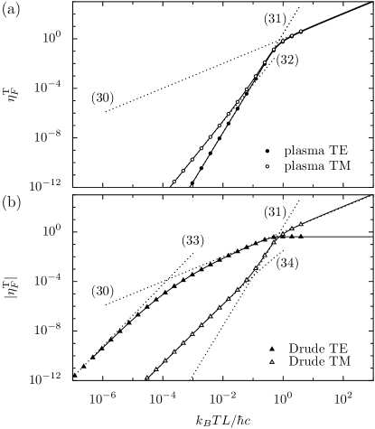
Figure 3: The thermal contribution to the factor $\eta_{F}$ defined in (28) for (a) the plasma model and (b) the Drude model is shown in terms of the dimensionless factor (29) as a function of the temperature for $\lambda_{P}/L=0.136$ and $\sigma_{0}=\sigma_{\text{Au}}$. The solid lines were obtained from the Lifshitz formula (26) while the filled and open symbols were obtained from (22) for the TE and TM mode, respectively. The thermal contribution of the TE mode within the Drude model is negative so that the absolute value of the data is shown. The dotted lines correspond to various low- and high-temperature approximations identified by the respective equation numbers. In (34), $C=-2.58$ was used.

Results for the plasma model are shown in Fig. 3a. The dotted lines indicate the high-temperature approximation

$$\eta_{F}^{T}=\frac{120}{\pi^{3}}L^{3}\mathbb{F}(0)\frac{k_{B}TL}{\hbar c}$$ (30)

as well as the low-temperature approximations for the TE mode

$$\eta_{F}^{T}=\frac{8}{3}\left(\frac{k_{B}TL}{\hbar c}\right)^{4}$$ (31)

and for the TM mode borda00 ; bezer02

$$\eta_{F}^{T}=\frac{240}{\pi^{3}}\zeta(3)\frac{c}{\omega_{P}L}\left(\frac{k_{B}TL}{\hbar c}\right)^{3}\,,$$ (32)

where the value of the Riemann zeta function is $\zeta(3)=1.202\ldots$ The expression (31) is independent of the plasma frequency and thus agrees with the leading thermal correction in the case of ideal mirrors sauer62 ; mehra67 ; schwi78 .

The temperature dependence of the Casimir force within the Drude model is depicted in Fig. 3b. The low-temperature approximations again shown as dotted lines differ from those of the plasma model. For the TE mode one finds

$$\eta_{F}^{T}=-\frac{15}{\pi^{4}}\left(\frac{\pi}{2}\right)^{1/2}\zeta\left(\frac{5}{2}\right)\left(\frac{L\sigma_{0}}{c}\right)^{3/2}\left(\frac{k_{B}TL}{\hbar c}\right)^{5/2}\,,$$ (33)

where $\zeta(5/2)=1.341\ldots$ The dependence on the material properties of the mirrors, i.e. in our case the plasma frequency and the relaxation frequency, enter here only through the dc conductivity (19). The fact that the prefactor increases with increasing conductivity indicates that the limit from the Drude to the plasma model is indeed nontrivial for the TE mode. This behavior is analogous to the low-temperature behavior (14) of the entropy of a free damped particle where the prefactor increases with decreasing damping constant.

The thermal correction (33) is negative and thereby reduces the zero-temperature Casimir force, thus already hinting at the fact that the TE modes will no longer contribute to the force at high temperatures. Accordingly, the thermal contribution $\eta_{F}^{T}$ for this mode saturates at $-\eta_{F}^{0}$, i.e. the negative of the zero-temperature contribution, so that the total force due to the TE modes vanishes in the high-temperature limit.

The expression (33) confirms the expression appearing as next-to-leading order in the low-temperature expansion of the free energy conjectured by Høye et al. hoye07 on the basis of an analysis of the Lifshitz formula footnote2 and later derived by Borel summation ellin08a . We will turn to the low-temperature behavior of the free energy in Sec. VI.

The low-temperature approximation for the TM mode

$$\eta_{F}^{T} =\frac{90}{\pi^{4}}(2\pi)^{1/2}\zeta\left(\frac{5}{2}\right)\left(\frac{c}{L\sigma_{0}}\right)^{1/2}\left(\frac{k_{B}TL}{\hbar c}\right)^{5/2}$$ (34)

$$\quad\times\left[\log\left(\hbar\omega_{P}/k_{B}T\right)+C\right]$$

is special because instead of a simple power law a logarithmic factor appears. $C$ is a constant for which (54) represents one contribution. As in (33), the material properties of the mirror appear in the prefactor only through the dc conductivity (19). In contrast to the TE mode, however, the prefactor decreases here with increasing conductivity so that the limit of infinite conductivity does not present difficulties. A derivation of (33) and (34) can be found in the appendix.

After multiplication of the low-temperature approximations (31), (32), (33), and (34) with the Casimir force for ideal mirrors at zero temperature (27) one notices that the leading thermal corrections to the force do not depend on the distance $L$ between the mirrors for the TE mode while they decrease as $1/L^{2}$ for the TM mode. The fact that the leading thermal correction for the TE mode is independent of $L$ does not mean, however, that at a fixed low temperature this contribution will survive for arbitrarily large separations of the two mirrors because an increase in $L$ will drive the system into the regime where the high-temperature approximation (30) applies. Then the Casimir force decreases as the mirrors are moved apart.

One feature visible in Fig. 3 for the parameters chosen here is still worth being noted. Both for the plasma model and the Drude model, the thermal contribution of the TM modes in an intermediate temperature regime increases with temperature according to the low-temperature behavior (31) of the TE modes for ideal mirrors. This happens because the thermal correction for the TM modes increases more slowly with temperature than for the TE mode in the presence of ideal mirrors. Before the high-temperature asymptote is reached, the thermal correction crosses over to the low-temperature behavior (31) of the TE mode in the ideal case or the plasma model. In this regime, the thermal corrections are dominated by the exponential factor in the closed-loop function (25) and the reflection constant can be set to one.

In Fig. 4 we show the total force expressed through the factor $\eta_{F}$ as a function of the temperature for $\lambda_{P}/L=0.136$ and the dc conductivity of gold. As in Fig. 3 the solid lines result from an evaluation of the Lifshitz formula (26) while the symbols represent data obtained by means of (22). Filled and open symbols correspond to TE and TM modes, respectively, while the grey symbols represent the sum of both. Circles and triangles correspond to the plasma and the Drude model, respectively. As noted before, the agreement between the two approaches (22) and (26) confirms the applicability of the Poisson resummation.

For the relatively small value of the relaxation frequency $\gamma$ chosen here, it is almost impossible for the TM modes to distinguish in Fig. 4 between the data corresponding to the Drude and plasma models. For these modes, the limit $\gamma\to 0$ continuously leads from the Drude to the plasma model. In contrast, the contribution of the TE modes behaves very differently for the Drude model and the plasma model. This difference survives the limit $\gamma\to 0$.

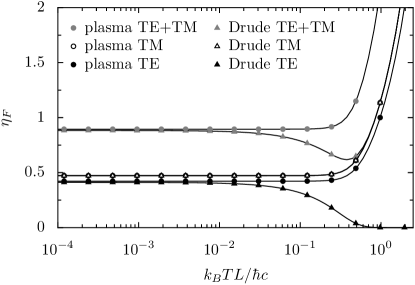
Figure 4: The total Casimir force is shown in terms of the dimensionless factor defined in (28) as a function of the temperature for $\lambda_{P}/L=0.136$ and $\sigma_{0}=\sigma_{\text{Au}}$. The lines were obtained from the Lifshitz formula (26) while the symbols represent data obtained from (22) for the plasma model (circles) and the Drude model (triangles). Filled and open symbols correspond to TE and TM modes, respectively, while grey symbols represent the sum of both modes. For the TM mode, because of the small relaxation frequency, the curves and symbols for the two models lie almost exactly on top of each other.

So far, an experimental distinction between the plasma and the Drude model is only based on an effectively zero-temperature measurement of the Casimir force decca07 . This quantity integrates over the closed-loop function and one therefore has to rely on quantitative comparisons. Thermal contributions to the Casimir force at low temperatures, on the other hand, are particularly sensitive to the low-frequency behavior of the closed-loop function and allow for a decision in favor of one or the other model already on a qualitative level. One of the indicators would evidently be the sign of the thermal correction. In addition, because of the different exponent in the low-temperature expressions (31) and (33) of the TE mode, thermal corrections for the Drude model should be visible already at lower temperatures or smaller mirror separation than expected for the plasma model.

V The transverse electric mode

We will now focus on the TE mode. To avoid cumbersome notation, it will be understood that all quantities refer to the TE mode even if this is not made explicit. In order to analyze the difference in behavior for the plasma model on the one hand and the Drude model on the other hand, it is appropriate to consider the difference in the thermal contributions to the factor $\eta_{F}$ defined in (28)

$$\Delta\eta_{F}^{T}=\eta_{F}^{T}(\text{Drude})-\eta_{F}^{T}(\text{plasma})\,.$$ (35)

To understand the transition from the Drude to the plasma model, it is crucial to realize that the closed-loop function $f(i\xi,i\kappa)$ for the Drude model depends only on the ratio $\xi/\gamma$. According to (20) and (25), the frequency enters only through the combination $\xi^{2}[1-\varepsilon(i\xi)]$, so that our assertion immediately follows from the relative permittivity (18) of the Drude model.

This behavior is illustrated in Fig. 5 where in the upper panel $-(\kappa L)^{2}\Delta f_{\text{TE}}$ is plotted as a function of $c\kappa/\omega_{P}$ and $\xi/\gamma$. In analogy to (35), $\Delta f_{\text{TE}}$ refers to the difference in the closed-loop functions of the TE mode within the Drude and the plasma model. The plotted quantity then describes the change of the integrand in (23) when going from the plasma model to the Drude model.

Figure 5b depicts $-L^{3}\Delta\mathbb{F}_{\text{TE}}(\xi)$ which according to (23) is obtained from the quantity shown in Fig. 5a by integration over $\kappa$. Due to the lower integration limit, $\mathbb{F}_{\text{TE}}$ for the Drude model and thus $\Delta\mathbb{F}_{\text{TE}}$ depend on $\gamma$. The dotted and dashed lines correspond to $L\gamma/c=10^{-1}$ and $10^{-3}$, respectively, while the solid line represents the limit $\gamma\to 0$. In agreement with the reasoning above, the low-frequency region, where this function has its largest weight, turns out to be practically independent of $\gamma$ as long as the relaxation frequency is not too large. Only at higher frequencies, finite relaxation frequencies lead to a rather sharp cutoff. With decreasing relaxation frequency, also the high-frequency part approaches more and more the decay with $1/\xi$ found in the limit $\gamma\to 0$.

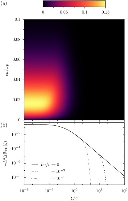
Figure 5: (a) The difference $-(\kappa L)^{2}\Delta f_{\text{TE}}$ between the integrands appearing in (23) for the Drude and the plasma model is shown as a function of $\xi/\gamma$ and $c\kappa/\omega_{P}$ for $\lambda_{P}/L=0.136$. (b) After integration over $\kappa$, one finds $-L^{3}\Delta\mathbb{F}_{\text{TE}}(\xi)$ which tends to the solid line in the limit $\gamma\to 0$. The dashed and dotted lines refer to $L\gamma/c=10^{-3}$ and $10^{-1}$, respectively.

In view of this observation, it is appropriate to rescale the frequency in (29) by $\gamma$ which implies that the temperature only appears in the combination $\hbar\beta\gamma$. The change (35) in the thermal contribution to the factor $\eta_{F}$ then turns into

$$\begin{split}\Delta\eta_{F}^{T}&=\frac{240}{\pi^{4}}\left(\frac{L\omega_{P}}{c}\right)^{3}\frac{L\gamma}{c}\sum_{n=1}^{\infty}\int_{0}^{\infty}dx\cos(n\hbar\beta\gamma x)\\ &\quad\times\int_{(\gamma/\omega_{P})x}^{\infty}du\,u^{2}\left[f^{D}\left(i\gamma x,i\frac{\omega_{P}}{c}u\right)-f^{P}\left(i\frac{\omega_{P}}{c}u\right)\right]\end{split}$$ (36)

where $u=c\kappa/\omega_{P}$ and $f^{D}$ and $f^{P}$ are the closed-loop functions (25) with the reflection coefficients of the Drude and plasma model, respectively.

In the limit of small $\gamma$, the lower limit of the inner integral in (36) effectively becomes zero. Then, the difference of the thermal corrections can be expressed as

$$\Delta\eta_{F}^{T}=\gamma g_{F}(\hbar\beta\gamma)\,.$$ (37)

In the special cases of Eqs. (30) and (33) we have $g_{F}(x)\sim 1/x$ and $g_{F}(x)\sim 1/x^{5/2}$, respectively. The prefactor $\gamma$ in (37) ensures that the sum appearing in (36) has a well-defined high-temperature limit.

As the temperature appears in (37) only in the combination $\hbar\beta\gamma$, it follows that the limits of zero temperature and zero relaxation frequency do not commute. For any finite temperature, the limit $\gamma\to 0$ implies $\hbar\beta\gamma\to 0$ so that (35) takes its classical value

$$\Delta\eta_{F}^{T}(\gamma=0)=-\frac{120}{\pi^{3}}\left(\frac{L\omega_{P}}{c}\right)^{3}\frac{L}{\hbar\beta c}\int_{0}^{\infty}du\,u^{2}f_{P}\left(i\frac{\omega_{P}}{c}u\right)\,.$$ (38)

This result is independent of the closed-loop function of the Drude model because the reflection coefficient within this model vanishes at zero frequency.

The implications of the behavior of $\Delta\eta_{F}^{T}$ can be understood with the help of Fig. 6 where the solid line representing $-\Delta\eta_{F}^{T}$ displays a smooth crossover between $-\eta_{F}^{T}(\text{plasma})$ (dotted line) at high temperatures and $\eta_{F}^{T}(\text{Drude})$ (dashed line) at low temperatures. Here, three different regimes can be distinguished which are indicated in Fig. 6 by the letters A–C. Regime A corresponds to high temperatures where to leading order in the temperature $-\eta_{F}^{T}(\text{plasma})$ agrees with the high-temperature behavior (38). As the thermal corrections within the plasma model turn to their low-temperature behavior described by (31) and thus decrease very fast with decreasing temperature, one reaches the regime B. Here, $\Delta\eta_{F}^{T}$ determines the thermal corrections of the Drude model which for sufficiently small relaxation frequency $\gamma$ are still given by the right-hand side of (38).

Figure 6: The absolute value of the difference of the thermal corrections (36) to the factor $\eta_{F}$ for the Drude and the plasma model is shown as a function of the temperature as solid line for $\lambda_{P}/L=0.136$ and $\sigma_{0}=\sigma_{\text{Au}}$. The dashed line represents the negative thermal correction for the Drude model while the dotted line corresponds to the thermal correction for the plasma model. A, B, and C indicate three different regimes discussed in the text.

Deviations from the high-temperature behavior occur at small temperatures which decrease with decreasing $\gamma$. It is found in the appendix that there $\Delta\eta_{F}^{T}\sim T^{5/2}$ with the prefactors given in (33). As the corresponding exponent for the plasma model is larger, it follows that also in regime C $\Delta\eta_{F}^{T}$ agrees with the thermal corrections for the TE mode within the Drude model. We remark that the scenario described here holds for sufficiently small values of $\gamma$. If the relaxation frequency is significantly larger than the plasma frequency $\omega_{P}$, an additional regime can appear as was the case in Fig. 3 for the TM mode. In an intermediate temperature regime, $\Delta\eta_{F}^{T}$ then follows the low-temperature behavior (31) of the plasma model.

In this section, we have identified a quantity, $\Delta\eta_{F}^{T}$, which depends on temperature only through the dimensionless quantity $\hbar\beta\gamma$. Although this quantity describes the difference between two different models, the Drude and the plasma models, it nevertheless directly determines $\eta_{F}^{T}$ for the Drude model at low temperatures where $\eta_{F}^{T}$ for the plasma model in view of the strong temperature dependence (31) becomes negligibly small. In the regions B and C of Fig. 6, the temperature dependence of $\eta_{F}^{T}$ for the Drude model is therefore analogous to that of thermodynamic quantities like the entropy of a free Brownian particle. As the relaxation frequency $\gamma$ decreases, the region B extends increasingly farther down to low temperatures. Nevertheless, below a temperature of the order of $\hbar\gamma/k_{B}$ a region C is always reached where the low-temperature behavior (33) applies. For any nonvanishing relaxation frequency, the situation is therefore different from the case $\gamma=0$. There, $\Delta\eta_{F}^{T}$ simply vanishes because setting $\gamma$ to zero in the Drude model will turn it into the plasma model.

VI Contribution of the transverse electric mode to the entropy

We now explore how the findings in the previous section translate to the free energy and in particular the entropy which is in the focus of the discussion about a possible violation of the third law of thermodynamics.

The entropy can be obtained by means of the standard thermodynamic relation

$$S=-\frac{\partial\mathcal{F}}{\partial T}$$ (39)

where $\mathcal{F}$ is the free energy

$$\mathcal{F} =\frac{\hbar A}{2\pi^{2}}\sum_{n=0}^{\infty}{}^{\prime}\int_{0}^{\infty}d\xi\cos(n\hbar\beta\xi)$$ (40)

$$\quad\times\int_{\xi/c}^{\infty}d\kappa\,\kappa\log\left[1-r^{2}(i\xi,i\kappa)\exp(-2\kappa L)\right]\,.$$

A Matsubara sum corresponding to (26) can be derived by means of a Poisson resummation. The Casimir force and the free energy are related by $F=-\partial\mathcal{F}/\partial L$. Comparing the structure of (22) and (40), it is clear that the reasoning of Sec. V can readily be applied to the free energy. In particular, the difference between the free energies in the Drude and plasma model is also of the form $\Delta\mathcal{F}=\gamma g_{E}(\hbar\beta\gamma)$. As for the force, this difference equals the result of the Drude model at low temperatures and thus the scaling can readily be verified for the leading low-temperature terms in the Drude model

$$\eta_{E}^{T} =-\frac{15}{\pi^{2}}[2\log(2)-1]\frac{L\sigma_{0}}{c}\left(\frac{k_{B}TL}{\hbar c}\right)^{2}$$ (41)

$$\quad-\frac{45}{2\pi^{4}}(2\pi)^{1/2}\zeta\left(\frac{5}{2}\right)\left(\frac{L\sigma_{0}}{c}\right)^{3/2}\left(\frac{k_{B}TL}{\hbar c}\right)^{5/2}+\ldots$$

which agrees with results derived earlier brevi04 ; hoye07 on the basis of the Lifshitz formula for the free energy. In analogy to the force, we have divided in $\eta_{E}^{T}$ the free energy at temperature $T$ by the free energy

$$\mathcal{F}_{\text{Cas}}=-\frac{\pi^{2}\hbar c}{720L^{3}}$$ (42)

at zero temperature for ideal mirrors and accounting for both polarizations. Without the normalization, the first term in (41) is independent of the mirror separation $L$ and thus does not contribute to the Casimir force. Therefore, it is the second term which corresponds to the leading low-temperature behavior (33) of the TE mode within the Drude model.

For the difference $\Delta S_{\text{TE}}$ of entropies in the Drude and plasma model one finds after taking the derivative of the difference $\Delta\mathcal{F}_{\text{TE}}$ of free energies with respect to temperature that it can be written in the form $\Delta S_{\text{TE}}/k_{B}=(\hbar\beta\gamma)^{2}g_{E}{}^{\prime}(\hbar\beta\gamma)/\hbar$. Here the prime indicates a derivative with respect to the argument of the function. As before for the force, we see that the limit $\gamma\to 0$ leads into the high-temperature regime. For any finite $\gamma$ there is however always a low-temperature regime determined by (41) which ensures that the entropy goes to zero as temperature goes to zero.

The temperature dependence of the entropy is illustrated in Figs. 7 and 8. Fig. 7 shows the contribution of the TE mode to the entropy for the Drude model with $\lambda_{P}/L=0.136$ and $L\gamma/c=0.01,0.1,1,10,100,1000$ from the lowest to the uppermost curve. These curves demonstrate that the dependence of $\Delta S_{\text{TE}}$ on the dimensionless temperature $\hbar\beta\gamma$ indeed applies to the contribution of the TE mode to the entropy in the Drude model for low temperatures where the entropy within the plasma model is negligible.

Figure 7: The contribution of the TE modes to the entropy is shown as a function of the temperature for the Drude model with $\lambda_{P}/L=0.136$ and $L\gamma/c=0.01,0.1,1,10,100,1000$ from bottom to top.

In Fig. 8 the solid lines show the total entropy for the same parameters as used in Fig. 7. In addition, the dashed line represents the contribution of the TM mode for $L\gamma/c=1000$ and the dotted line gives the total entropy for the plasma model with $\lambda_{P}=0.136$. For small relaxation frequencies $\gamma$, the temperature dependence of the entropy displays the same qualitative behavior as found for the specific case of copper plates bostr04 . In particular, a temperature regime exists where the entropy becomes negative. In any case, however, the entropy will go to zero as temperature goes to zero, in accordance with Nernst’s theorem. Furthermore, it can be seen that the total entropy remains positive if $\gamma$ is sufficiently large. This is the case for $L\gamma/c=1000$, i.e. the uppermost curve in Fig. 8. The comparison with the corresponding contribution from the TM mode depicted as dashed line shows that the contribution of the TE mode is nevertheless negative.

Figure 8: The total entropy is shown as a function of the temperature for the Drude model with $\lambda_{P}/L=0.136$ and $L\gamma/c=0.01,0.1,1,10,100,1000$ (solid line, from bottom to top). The dashed line indicates the contribution of the TM mode for $L\gamma/c=1000$ and the dotted line corresponds to the entropy obtained for the plasma model. In contrast to Fig. 7, temperature is taken with respect to the mirror separation $L$.

With increasing relaxation frequency or, equivalently, decreasing conductivity, the electromagnetic field couples less strongly to the electrons in the mirrors and in the limit of vanishing conductivity the electromagnetic field could be considered as an isolated system. In this situation, the entropy has to remain positive as in fact it does. If, on the other hand, the coupling is strong, the electromagnetic field represents only a subsystem whose entropy can well become negative as has already been pointed out in Ref. hoye03, .

Letting $\gamma$ formally go to zero in the low-temperature expression for the entropy would in principle lead to a nonvanishing negative entropy at zero temperature, but then we would have to start with the plasma model from the very beginning where it is generally agreed that Nernst’s theorem holds. The noncontinuous transition from the Drude model to the plasma model thus makes it possible that in the first case for nonvanishing values of $\gamma$ and in the second case for $\gamma=0$ the entropy goes to zero in the zero-temperature limit as it should.

VII Conclusions

We have considered the thermodynamics of a free damped quantum particle on the one hand and of the electromagnetic field enclosed between two mirrors of finite conductivity, on the other hand. If in the first case the normalization volume is very large and in the second case the plasma frequency and the frequency $c/L$ associated with the mirror separation $L$ are large compared to the relaxation frequency of the Drude-type mirrors, the temperature dependence in both cases is dominated by the interplay of two energy scales: the thermal energy $k_{B}T$ and the energy $\hbar\gamma$ associated with the damping or the relaxation present in a Drude metal.

In such a situation, the limits of zero temperature and zero damping do not commute. For any finite temperature, the limit of small damping or relaxation will restore the classical high-temperature behavior. This behavior, if continued down to zero temperature, could potentially violate requirements imposed by thermodynamics. However, for any nonvanishing damping, there exists a quantum regime at low temperatures, which regularizes the approach to zero temperature so that no problems with Nernst’s theorem arise. For room-temperature measurements on the Casimir effect with metallic mirrors made of gold, the ratio $k_{B}T/\hbar\gamma$ is close to one, placing these experiments into the transition region between the classical and the quantum regime.

The Casimir effect with its strong coupling between the electromagnetic field modes and the metallic mirrors is a prime example where the coupling between system and environment is far from negligible. In such cases, the coupling will affect the thermodynamic properties in the quantum regime and even lead to negative values for the entropy or the specific heat at low temperatures. Such negative values result from the restriction to a subsystem and are therefore not in contradiction with thermodynamic principles. The appearance of a negative entropy or specific heat is not specific to the free Brownian quantum particle hangg08 and the Casimir effect hoye03 but is also known for example in condensed matter physics flore04 ; zitko08 .

While there exists a direct analogy in the low-temperature behavior of the free Brownian particle and the Casimir effect, there is an apparent difference at high temperatures. In the first case, the limit of vanishing damping leads to the free particle while in the second case, even in the limit of vanishing relaxation frequency, the TE mode contributes within the plasma model while it does not for the Drude model. This is a consequence of the fact that the quantity which enters the analogy for the Casimir effect is not the Casimir force itself but the difference of the Casimir forces in the Drude and the plasma model. It is this difference which in the classical limit becomes independent of the relaxation frequency and thus within our analogy accounts for the suppression of the Casimir force by a factor of two at high temperatures.

Appendix A Low-temperature expressions for the Casimir force within the Drude model

In the following, we derive the low-temperature expansions (33) and (34) for the TE and TM modes, respectively, within the Drude model. We take as our starting point the expressions (23) and (29). In view of our discussion in Sec. V, we introduce a dimensionless frequency $x=\xi/\gamma$. As we are interested in the low-temperature behavior and therefore in the behavior of $\mathbb{F}(x)$ for small $x$, it is convenient to introduce another dimensionless variable $u=(c\kappa/\omega_{P})(1+1/x)^{1/2}$. We thus bring (29) into the form

$$\eta_{F}^{T} =\frac{240}{\pi^{4}}\frac{L^{4}\omega_{P}^{3}\gamma}{c^{4}}\sum_{n=1}^{\infty}\int_{0}^{\infty}dx\cos(n\hbar\beta\gamma x)\left(\frac{x}{x+1}\right)^{3/2}$$ (43)

$$\quad\times\int_{u_{0}}^{\infty}du\,u^{2}\frac{r_{p}^{2}(u)}{\exp\left[\frac{2L\omega_{P}}{c}\left(\frac{x}{x+1}\right)^{1/2}u\right]-r_{p}^{2}(u)}$$

with

$$u_{0}=\frac{\gamma}{\omega_{P}}[x(x+1)]^{1/2}\,.$$ (44)

For the TE mode, the behavior of the integrand for small $x$ is dominated by the factor $x^{3/2}$ in front of the integral over $u$. The lower limit of integration (44) of that integral can then be set to zero and in its integrand, the reflection coefficient $r_{\text{TE}}(u)$ varies rapidly compared to the exponential function. To leading order, we are therefore left with

$$\eta_{F}^{T} =\frac{240}{\pi^{4}}\left(\frac{L\omega_{P}}{c}\right)^{3}\frac{L\gamma}{c}\sum_{n=1}^{\infty}\int_{0}^{\infty}dx\cos(n\hbar\beta\gamma x)x^{3/2}$$ (45)

$$\quad\times\int_{0}^{\infty}du\,u^{2}\frac{r_{\text{TE}}(u)^{2}}{1-r_{\text{TE}}(u)^{2}}$$

where

$$r_{\text{TE}}(u)=\frac{(u^{2}+1)^{1/2}-u}{(u^{2}+1)^{1/2}+u}\,.$$ (46)

The two integrals can be carried out yielding

$$\int_{0}^{\infty}du\,u^{2}\frac{r_{\text{TE}}(u)^{2}}{1-r_{\text{TE}}(u)^{2}}=\frac{1}{12}$$ (47)

and

$$\int_{0}^{\infty}dx\cos(x)x^{3/2}=-\frac{3}{8}(2\pi)^{1/2}\,.$$ (48)

In the latter integral, an infinitely weak exponential regularization was assumed. Inserting these two results into (45) one finds the leading low-temperature contribution (33) of the TE mode to the Casimir force.

We now turn to the TM mode. In contrast to the TE mode, the absolute value of the reflection coefficient equals one in the limit of small frequencies, in which we are interested in order to obtain the low-temperature behavior. We separate the closed-loop function into two contributions

$$f_{\text{TM}}(i\xi,i\kappa)=f_{\text{TM}}^{(1)}(i\kappa)+f_{\text{TM}}^{(2)}(i\xi,i\kappa)$$ (49)

with

$$f_{\text{TM}}^{(1)}(i\kappa)=\frac{1}{\exp(2\kappa L)-1}$$ (50)

and

$$f_{\text{TM}}^{(2)}(i\xi,i\kappa)=\frac{\exp(2\kappa L)[r_{\text{TM}}^{2}(i\xi,i\kappa)-1]}{[\exp(2\kappa L)-1][\exp(2\kappa L)-r_{\text{TM}}^{2}(i\xi,i\kappa)]}\,.$$ (51)

The first contribution is familiar from the case of ideal mirrors and leads to a low-temperature contribution of the form (31) which goes with $T^{4}$. The second term will turn out to increase more slowly with temperature and therefore determines the leading-order term. For small values of the dimensionless variables $x$ and $u$, one obtains to leading order

$$u^{2}f_{\text{TM}}^{(2)}=-\left(\frac{c\gamma}{\omega_{P}^{2}L}\right)^{2}\frac{1}{u}\,.$$ (52)

The leading term of the thermal correction to the factor $\eta_{F}$ thus becomes

$$\eta_{F}^{T} =-\frac{240}{\pi^{4}}\left(\frac{L\gamma}{c}\right)^{3}\frac{\gamma}{\omega_{P}}\sum_{n=1}^{\infty}\int_{0}^{\infty}dx\cos(n\hbar\beta\gamma x)x^{3/2}$$ (53)

$$\quad\times\int_{\gamma x/\omega_{P}}^{\infty}du\frac{1}{u}\,.$$

The integral over $u$ yields a logarithmic contribution from the lower limit of integration. Such a logarithmic term also appears in the evaluation of the low-temperature behavior of the TM mode in the plasma model borda00 , even though the final result only contains a power of temperature. In contrast, here, the logarithmic term will survive the integration over $x$. The ultraviolet behavior of the integral over $u$ will be regularized if the complete closed-loop function is taken into account. From here, a contribution to the next-to-leading term can be expected.

Together with (48), one finds for (53) the low-temperature approximation (34) with the constant

$$C =\frac{1}{\zeta(5/2)}\sum_{n=1}^{\infty}\frac{\log(n)}{n^{5/2}}$$ (54)

$$\quad+\frac{8}{3(2\pi)^{1/2}}\int_{0}^{\infty}dy\cos(y)y^{3/2}\log(y)$$

which has a numerical value $C\approx 1.155$. Note, however, that we have neglected terms which potentially contribute to this constant.

References

- (1) P. Hänggi and G.-L. Ingold, Acta Phys. Pol. B 37, 1537 (2006).
- (2) C. Hörhammer and H. Büttner, J. Stat. Phys. 133, 1161 (2008).
- (3) M. Bandyopadhyay, arXiv:0804.0290.
- (4) P. Hänggi, G.-L. Ingold, and P. Talkner, New J. Phys. 10, 115008 (2008).
- (5) C.-Y. Wang and J.-D. Bao, Chin. Phys. Lett. 25, 429 (2008).
- (6) J. Kumar, P. A. Sreeram, and S. Dattagupta, Phys. Rev. E 79, 021130 (2009).
- (7) G.-L. Ingold, P. Hänggi, and P. Talkner, arXiv:0811.3509.
- (8) M. Bandyopadhyay and S. Dattagupta, arXiv:0903.2952.
- (9) M. Bordag, U. Mohideen, and V. M. Mostepanenko, Phys. Rep. 353, 1 (2001).
- (10) K. A. Milton, J. Phys. A: Math. Gen. 37, R209 (2004).
- (11) R. G. Barrera and S. Reynaud (eds.), Focus on Casimir Forces, New J. Phys. 8, 234–244 (2006).
- (12) A. Lambrecht, P. A. Maia Neto, and S. Reynaud, New J. Phys. 8, 243 (2006).
- (13) H. B. G. Casimir, Proc. K. Ned. Akad. Wet. 51, 793 (1948).
- (14) R. S. Decca, D. López, E. Fischbach, G. L. Klimchitskaya, D. E. Krause, and V. M. Mostepanenko, Phys. Rev. D 75, 077101 (2007). For modern experiments prior to 2007, see references therein.
- (15) J. N. Munday and F. Capasso, Phys. Rev. A 75, 060102(R) (2007).
- (16) H. B. Chan, Y. Bao, J. Zou, R. A. Cirelli, F. Klemens, W. M. Mansfield, and C. S. Pai, Phys. Rev. Lett. 101, 030401 (2008).
- (17) P. J. van Zwol, G. Palasantzas, and J. Th. M. De Hosson, Phys. Rev. B 77, 075412 (2008).
- (18) J. N. Munday, F. Capasso, and V. A. Parsegian, Nature 457, 170 (2009).
- (19) G. Jourdan, A. Lambrecht, F. Comin, and J. Chevrier, EPL 85, 31001 (2009).
- (20) M. Masuda and M. Sasaki, Phys. Rev. Lett. 102, 171101 (2009).
- (21) S. de Man, K. Heeck, R. J. Wijngaarden, and D. Iannuzzi, arXiv:0901.3720.
- (22) G. L. Klimchitskaya and V.M. Mostepanenko, Contemp. Phys. 47, 131 (2006).
- (23) I. Brevik, S. A. Ellingsen, and K. A. Milton, New J. Phys. 8, 236 (2006).
- (24) K. A. Milton, J. Phys.: Conf. Ser. 161, 012001 (2009).
- (25) J. R. Torgerson and S. K. Lamoreaux, Phys. Rev. E 70, 047102 (2004).
- (26) T. Dittrich, P. Hänggi, G.-L. Ingold, B. Kramer, G. Schön, and W. Zwerger, Quantum transport and dissipation, Chap. 4 (Wiley-VCH, Weinheim, 1998).
- (27) U. Weiss, Quantum dissipative systems (World Scientific, Singapore, 1999).
- (28) G.-L. Ingold, Lect. Notes Phys. 611, 1 (2002).
- (29) H. Grabert, P. Schramm, and G.-L. Ingold, Phys. Rep. 168, 115 (1988).
- (30) A. O. Caldeira and A. J. Leggett, Ann. Phys. (N.Y.) 149, 374 (1983).
- (31) H. Grabert, U. Weiss, and P. Talkner, Z. Phys. B 55, 87 (1984).
- (32) G. W. Ford, J. T. Lewis, and R. F. O’Connell, Phys. Rev. Lett. 55, 2273 (1985).
- (33) In the context of dissipative quantum system, this choice of the damping kernel is usually referred to as Drude model. To avoid confusion with the Drude model for metals, we do not employ this term here.
- (34) C. Genet, A. Lambrecht, and S. Reynaud, Phys. Rev. A 62, 012110 (2000).
- (35) For a discussion of the low-temperature behavior of the relaxation frequency see G. L. Klimchitskaya and V. M. Mostepanenko, Phys. Rev. E 77, 023101 (2008) and J. S. Høye, I. Brevik, S. A. Ellingsen, and J. B. Aarseth, Phys. Rev. E 77, 023102 (2008).
- (36) A. Lambrecht and S. Reynaud, Eur. Phys. J. D 8, 309 (2000).
- (37) V. B. Svetovoy, P. J. van Zwol, G. Palasantzas, and J. Th. M. De Hosson, Phys. Rev. B 77, 035439 (2008).
- (38) V. B. Svetovoy, Phys. Rev. A 76, 062102 (2007).
- (39) S. A. Ellingsen, Phys. Rev. E 78, 021120 (2008).
- (40) M. Boström and B. E. Sernelius, Phys. Rev. Lett. 84, 4757 (2000).
- (41) B. Jancovici and L. Šamaj, Europhys. Lett. 72, 35 (2005).
- (42) P. R. Buenzli and Ph. A. Martin, Europhys. Lett. 72, 42 (2005).
- (43) G. Bimonte, Phys. Rev. A 79, 042107 (2009).
- (44) M. T. Jaekel and S. Reynaud, J. Phys. I (France) 1, 1395 (1991).
- (45) C. Genet, A. Lambrecht, and S. Reynaud, Phys. Rev. A 67, 043811 (2003).
- (46) S. Reynaud, A. Lambrecht, and C. Genet, in: Proceedings of the 6th Workshop on Quantum Field Theory Under the Influence of External Conditions, edited by K. A. Milton (Rinton Press, Princeton, 2004), p. 36–43.
- (47) E. M. Lifshitz, Sov. Phys. JETP 2, 73 (1956).
- (48) J. S. Høye, I. Brevik, S. A. Ellingsen, and J. B. Aarseth, Phys. Rev. E 75, 051127 (2007).
- (49) S. A. Ellingsen, I. Brevik, J. S. Høye, and K. A. Milton, Phys. Rev. E 78, 021117 (2008).
- (50) I. Brevik, S. A. Ellingsen, J. S. Høye, and K. A. Milton, J. Phys. A: Math. Theor. 41, 164017 (2008).
- (51) M. Bordag, B. Geyer, G. L. Klimchitskaya, and V. M. Mostepanenko, Phys. Rev. Lett. 85, 503 (2000).
- (52) V. B. Bezerra, G. L. Klimchitskaya, and V. M. Mostepanenko, Phys. Rev. A 66, 062112 (2002).
- (53) F. Sauer, Ph.D. thesis (Göttingen, 1962).
- (54) J. Mehra, Physica 37, 145 (1967).
- (55) J. Schwinger, L. L. DeRaad, Jr., and K. A. Milton, Ann. Phys. (N.Y.) 115, 1 (1978).
- (56) In order to relate (33) to the expression in the appendix A of ref. hoye07, note that .
- (57) I. Brevik, J. B. Aarseth, J. S. Høye and K. A. Milton, in: Proceedings of the 6th Workshop on Quantum Field Theory Under the Influence of External Conditions, edited by K. A. Milton (Rinton Press, Princeton, 2004) pp. 54–65.
- (58) M. Boström and B. E. Sernelius, Physica A 339, 53 (2004).
- (59) J. S. Høye, I. Brevik, J. B. Aarseth, and K. A. Milton, Phys. Rev. E 67, 056116 (2003).
- (60) S. Florens and A. Rosch, Phys. Rev. Lett. 92, 216601 (2004).
- (61) R. Žitko and T. Pruschke, Phys. Rev. B 79, 012507 (2009).