A conjugate gradient method for the solution of the non–LTE line radiation transfer problem

This study concerns the fast and accurate solution of the line radiation transfer problem, under non-LTE conditions. We propose and evaluate an alternative iterative scheme to the classical ALI-Jacobi method, and to the more recently proposed Gauss-Seidel and Successive Over-Relaxation (GS/SOR) schemes. Our study is indeed based on the application of a preconditioned bi-conjugate gradient method (BiCG-P). Standard tests, in 1D plane parallel geometry and in the frame of the two-level atom model, with monochromatic scattering, are discussed. Rates of convergence between the previously mentioned iterative schemes are compared, as well as their respective timing properties. The smoothing capability of the BiCG-P method is also demonstrated.

1 Introduction

The solution of the radiative transfer equation, under non–LTE conditions, is a classical problem in astrophysics. Many numerical methods have been used since the beginning of the computer era, from difference equations methods (e.g., Feautrier 1964, Cuny 1967, Auer & Mihalas 1969) to iterative schemes (e.g., Cannon 1973, Scharmer 1981, Olson et al. 1986).

Since the seminal paper of Olson et al. (1986), the so-called ALI or Accelerated $\Lambda$-Iteration scheme is nowadays one of the most popular method for solving complex radiation transfer problems. Using as approximate operator the diagonal of the $\Lambda$ operator (see e.g., Mihalas 1978), it is a Jacobi iterative scheme. It has been generalized for multilevel atom problems (Rybicki & Hummer 1991), multi-dimensional geometries (Auer & Paletou 1994, Auer et al. 1994, van Noort et al. 2002), and polarized radiation transfer (e.g., Faurobert et al. 1997, Trujillo Bueno & Manso Sainz 1999).

Despite the many success of the ALI method, Trujillo Bueno & Fabiani Bendicho (1995) proposed a novel iterative scheme for the solution of non–LTE radiation transfer. They adapted Gauss-Seidel and Successive Over-Relaxation (GS/SOR) iterative schemes, well-known in applied mathematics as being superior, in terms of convergence rate, to the ALI–Jacobi iterative scheme. It is interesting to note that, besides their application to radiation transfer, both Jacobi and GS/SOR iterative schemes were proposed during the xix^th century.

Conjugate gradient-like, hereafter CG-like, iterative methods were proposed more recently by Hestenes & Stiefel (1952). They are of a distinct nature than ALI-Jacobi and GS/SOR methods. Unlike the later, CG-like methods are so-called non-stationary iterative methods (see e.g., Saad 2008). Very few articles discussed its application to the radiation transfer equation (see e.g., Amosov & Dmitriev 2005) and, to the best of our knowledge, they have not been properly evaluated, so far, for astrophysical purposes.

Such an evaluation is the scope of the present research note. This alternative approach is relevant to the quest for ever faster and accurate numerical methods for the solution of the non–LTE line radiation transfer problem.

2 The iterative scheme

In the two-level atom case, and with complete frequency redistribution, the non-LTE line source function is usually written as

$$S(\tau)=(1-\varepsilon)\bar{J}(\tau)+\varepsilon B(\tau)\,,$$ (1)

where $\tau$ is the optical depth, $\varepsilon$ is the collisional destruction probability, $B$ is the Planck function and $\bar{J}$ is the usual mean intensity:

$$\bar{J}=\oint\displaystyle{{{d\Omega}\over{4\pi}}}\int_{-\infty}^{+\infty}{\phi_{\nu}I_{\nu\Omega}d\nu}\,,$$ (2)

where the optical depth dependence of the specific intensity $I_{\nu\Omega}$ (and, possibly, of the line absorption profile $\phi_{\nu}$) is omitted for simplicity.

The mean intensity is usually written as the formal solution of the radiative transfer equation

$$\bar{J}=\Lambda[S]\,,$$ (3)

or, in other terms, the solution of the radiation transfer equation for a known source function (see e.g., Mihalas 1978).

Let us define $A\equiv{\rm Id}-(1-\varepsilon)\Lambda$, the unknown $x\equiv S$ and the right-hand side $b\equiv\varepsilon B$. Then, the solution of the radiative transfer equation is equivalent to solving the system of equations:

$$Ax=b\,.$$ (4)

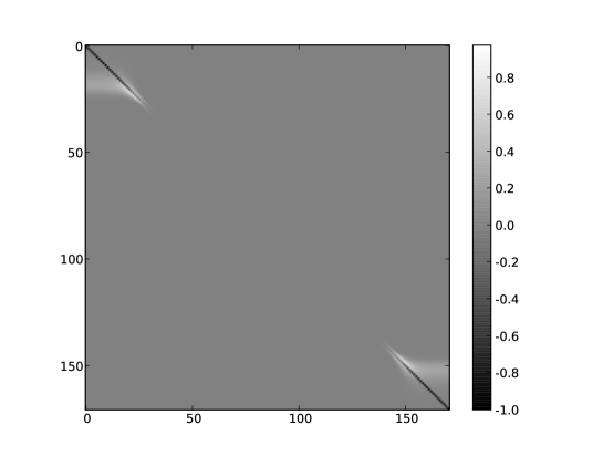
Figure 1: Typical structure of the $A$ operator, computed for the case of a self-emitting 1D, plane parallel finite slab. Such an operator is, more generally, non-symmetric positive definite. For the sake of getting a better contrast for the off-diagonal parts, we magnified the negative values of the original operator by a factor of 5, and we display in fact the opposite of the modified operator.

Among the various forms of CG-based methods, the bi-conjugate gradient (hereafter BiCG) method is more appropriate for the case of operators $A$ which are not symmetric positive definite. It is indeed the case for our radiative transfer problem, as illustrated in Fig. 1 where we display the structure of the operator $A$ for the case of a symmetric 1D grid of maximum optical depth $\tau_{\rm max}=2\times 10^{8}$, discretized with 8 spatial points per decade and using $\varepsilon=10^{-6}$.

A general description of the BiCG gradient method can be found in several classical textbooks of applied mathematics (see e.g., Saad 2008; it is important to note that this method requires the use of the transpose of the $A$ operator, $A^{T}$). However, the BiCG method remains efficient until the $A$ operator becomes very badly conditioned i.e., for very high albedo cases, typically when $\varepsilon<10^{-6}$. For the later cases, it is therefore crucial to switch to a more efficient scheme, using preconditioning of the system of equations.

Hereafter, we derive the algorithm for the BiCG method with preconditioning (hereafter BiCG-P). In such a case, one seeks instead for a solution of:

$$M^{-1}Ax=M^{-1}b\,,$$ (5)

where the matrix $M$ should be easy to invert. A “natural” choice for the non-LTE radiation transfer problem, is to precondition the system of equations with the diagonal of the full operator $A$.

From an initial guess for the source function, $x_{0}=S^{(0)}$, compute a residual $r_{0}$ such as:

$$r_{0}=b-Ax_{0}\,.$$ (6)

Set the second residual $\tilde{r}_{0}$ such that $(r_{0},\tilde{r}_{0})\neq 0$, where $(a,b)$ means the inner product between vectors $a$ and $b$. For all the cases considered by us, setting $r_{0}=\tilde{r}_{0}$ proved to be adequate.

Now, the BiCG-P algorithm consists in running until convergence the following iterative scheme, where $j$ is the iterative scheme index. The first steps consist in solving:

$$Mz_{j-1}=r_{j-1}\,,$$ (7)

and

$$M^{T}\tilde{z}_{j-1}=\tilde{r}_{j-1}\,.$$ (8)

These steps are both simple and fast to compute, since $M$ is a diagonal operator. Then one computes:

$$\rho_{j-1}=(z^{T}_{j-1},\tilde{r}_{j-1})\,.$$ (9)

If $\rho_{j-1}=0$ then the method fails, otherwise the algorithm continues with the following computations. If $j=1$ then, set $p_{j}=z_{j-1}$ and $\tilde{p}_{j}=\tilde{z}_{j-1}$. For $j>1$, compute:

$$\beta_{j-1}=\rho_{j-1}/\rho_{j-2}\,,$$ (10)

$$p_{j}=z_{j-1}+\beta_{j-1}p_{j-1}\,,$$ (11)

and:

$$\tilde{p}_{j}=\tilde{z}_{j-1}+\beta_{j-1}\tilde{p}_{j-1}\,.$$ (12)

Then make $q_{j}=Ap_{j}$ and $\tilde{q}_{j}=A^{T}\tilde{p}_{j}$, as well as:

$$\alpha_{j}={{\rho_{j-1}}\over{({\tilde{p}^{T}_{j}},{q_{j}})}}\,.$$ (13)

Finally, one advances the source function according to:

$$x_{j}=x_{j-1}+\alpha_{j}p_{j}\,,$$ (14)

and the two residuals:

$$r_{j}=r_{j-1}-\alpha_{j}q_{j}\,,$$ (15)

and,

$$\tilde{r}_{j}=\tilde{r}_{j-1}-\alpha_{j}\tilde{q}_{j}\,.$$ (16)

This process, from Eq. (7) to Eq. (16), is then repeated to convergence. We have found that a convenient stopping criterion is to interrupt the iterative process when:

$${{\|r\|_{2}}\over{\|b\|_{2}}}<10^{-2}\,.$$ (17)

Indeed, this stopping criterion guarantees that the floor value of the true error, defined in §3.1, is always reached.

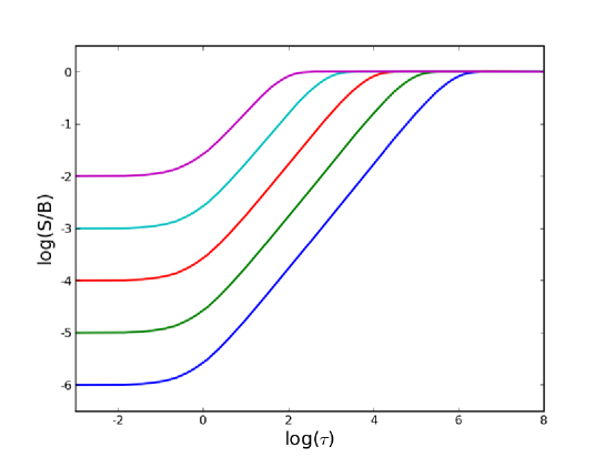
Figure 2: Solutions for the monochromatic scattering in an isothermal atmosphere, obtained for different values of $\varepsilon$, ranging from $10^{-4}$ to $10^{-12}$. Both the expected $\sqrt{\varepsilon}$ surface law and thermalisation lengths $\approx 1/\sqrt{\varepsilon}$ are perfectly recovered.

3 Results

The solution of the non–LTE radiative transfer problem for a constant property, plane-parallel 1D slab is a standard test for any new numerical method. Indeed, the so-called monochromatic scattering case allows a direct comparison of the numerical solutions to the analytical “solution”, $S_{\rm Edd}$, which can be derived in Eddington’s approximation (see e.g., the discussion in §5. of Chevallier et al. 2003).

3.1 Scaling laws for non-LTE source function solutions

In Fig. 2, we display the run of the source function with optical depth, for a self-emitting slab of total optical thickness $\tau_{\rm max}=2\times 10^{8}$, using a 9-point per decade spatial grid, a one-point angular quadrature with $\mu=\pm 1/\sqrt{3}$, and $\varepsilon$ values ranging from $10^{-4}$ to $10^{-12}$.

Both the $\sqrt{\varepsilon}$ surface law and thermalisation lengths $\approx 1/\sqrt{\varepsilon}$ are perfectly recovered, even for the numerically difficult cases of large ($a\lessapprox 1$) albedos.

The “true” error, that is:

$${T}_{e}={{\rm max}}\left({{\mid S^{(j)}-S_{{\rm Edd}}\mid}\over{S_{\rm Edd}}}\right)\,,$$ (18)

is displayed in Fig. 3, respectively for the GS, SOR and BiCG-P iterative schemes. SOR was used with a $\omega=1.5$ over-relaxation parameter, and $\varepsilon=10^{-12}$ in that case.

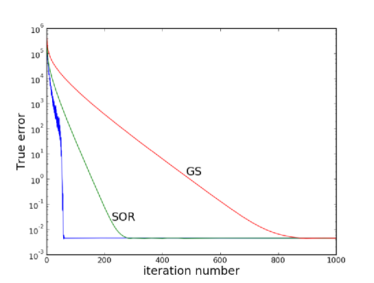
Figure 3: History of the true error vs. iteration number for $\varepsilon=10^{-12}$, respectively with Gauss-Seidel, SOR (with $\omega=1.5$) and BiCG-P with the diagonal of A as a preconditioner.

3.2 Timing properties

The typical timing properties of the BiCG-P scheme, for the cases considered here, are summarized in Table 1. While each GS/SOR iteration is about 20% longer than one ALI-iteration, the increase of time per iteration, with the number of depth points, for BiCG-P is significant. However, the balance between computing time and reduction of the number of iterations always remains in favour of the BiCG-P scheme vs. GS/SOR and, a fortiori, ALI.

Table 1: Timing properties of the BiCG-P iterative schemes, depending on the optical depth grid refinement expressed as the number of point per decade, N_τ, for a $\tau_{\rm max}=2\times 10^{8}$, and $\varepsilon=10^{-8}$ self-emitting slab. We use a time normalized to the time for a ALI-iteration. Note that GS/SOR is, in comparison, about 20% slower than ALI.

Nτ	5	8	11	14	17	20
t/tALI	0.85	1.2	1.8	2.1	2.3	2.7

3.3 Sensitivity to the spatial refinement

We adopted the same slab model as the one reported in the previous section, with $\varepsilon=10^{-8}$, and we allowed the grid refinement to vary from 5 to 20 points per decade, with a step of 3.

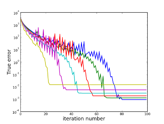
Figure 4: Evolution of the true error for varying spatial grid refinements, from 5 to 20 points per decade, with a step of 3. The value of the true error plateau decreases with an increasing grid refinement.

Figure 4 shows the sensitivity of the method with grid refinement. Increasing grid refinement corresponds to a decreasing value of the floor value of the true error, which demonstrates the need of a sufficient spatial resolution for the sake of accuracy on the numerical solutions. The number of iterative steps necessary to fulfill the stopping criterion defined in Eq. (17) is practically linear in the number of depth points.

3.4 Smoothing capability

A strong argument in favour of the Gauss-Seidel iterative scheme resides in its smoothing capability. This point is particularly important in the frame of multi-grid methods for the solution of non–LTE radiative transfer problems (see e.g., Fabiani Bendicho et al. 1997).

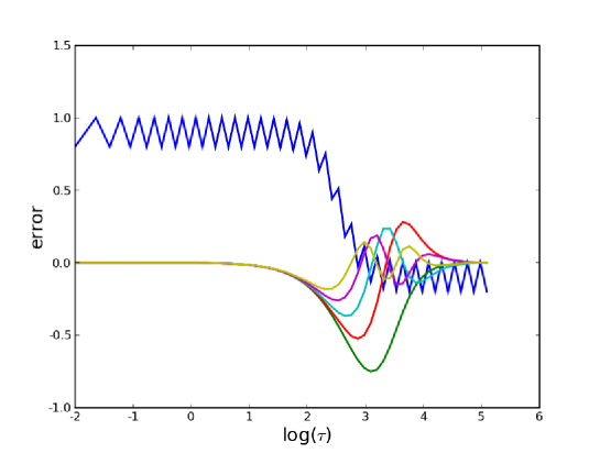
Figure 5: Initialization and evolution of the error, $S^{(j)}-S^{(\infty)}$, during the 5 first iterations of the BiCG-P scheme. The high-frequency component introduced ab initio in the source function is removed after the very first iteration of BiCG-P. Other curves, of continuously decreasing amplitudes, correspond to iterations 2 to 5.

We have reproduced the test initially proposed by Trujillo Bueno & Fabiani Bendicho (1995, see their Fig. 9) for the GS method. Here we consider a semi-infinite slab of maximum optical thickness $10^{5}$, sampled with a 9-point per decade grid, and $\varepsilon=10^{-6}$. The test consists in injecting ab initio a high-frequency component into the error, $S^{(0)}-S^{(\infty)}$, on the initial guess for the source function. In Fig. 5, the initial error we used is easily recognized as the hyperbolic tangent-like curve, to which a high-frequency component was added.

After the very first iterate of the BiCG-P iterative process, the error has an amplitude of $\approx 0.75$ and, more importantly, it is already completely smoothed. Other error curves displayed in Fig. 5, of continuously decreasing amplitudes, are the successive errors at iterates 2 to 5.

This simple numerical experiment demonstrates that BiCG-P can also be used as an efficient smoother for multi-grid methods.

4 Conclusion

We propose an alternative method for the solution of the non–LTE radiation transfer problem. Preliminary but standards tests for the two-level atom case in 1D plane parallel geometry are successful. In such a case, the timing properties of the preconditioned BiCG method are comparable to the ones of ALI, GS and SOR stationnary iterative methods. However the convergence rate of BiCG-P is signifiantly better.

The main potential drawback of the BiCG-P method is in the usage of the $A^{T}$ operator. A detailed trade-off analysis between such over-computing time and an improved convergence rate, with respect to the ones of GS/SOR iterative schemes, is currently being conducted.

Multi-level and multi-dimensional cases will be considered further. However, the use of BiCG-P does not require the cumbersome modifications of multi-dimensional formal solvers required by GS/SOR methods (see e.g., Léger et al. 2007).

- (1) Amosov, A.A. & Dmitriev, V.V. 2005, MPEI Bulletin, 6, 5 (in russian)
- (2) Auer, L.H. & Mihalas, D. 1969, ApJ, 158, 641
- (3) Auer, L.H. & Paletou, F. 1994, A&A, 285, 675
- (4) Auer, L.H., Fabiani Bendicho, P. & Trujillo Bueno, J. 1994, A&A, 292, 599
- (5) Cannon, C.J. 1973, ApJ, 185, 621
- (6) Chevallier, L., Paletou, F. & Rutily, B. 2003, A&A, 411, 221
- (7) Cuny, Y. 1967, Ann. Ap., 30, 143
- (8) Fabiani Bendicho, P., Trujillo Bueno, J. & Auer, L.H. 1997, A&A, 324, 161
- (9) Faurobert, M., Frisch, H. & Nagendra, K.N. 1997, A&A, 322, 896
- (10) Feautrier, P. 1964, C.R.A.S., 258, 3189
- (11) Hestenes, M.R. & Stiefel, E. 1952, Journal of Research of the National Bureau of Standards, 49(6), 409
- (12) Léger, L., Chevallier, L. & Paletou, F. 2007, A&A, 470, 1
- (13) Mihalas, D. 1978, Stellar Atmospheres (San Francisco: Freeman)
- (14) Olson, G.L., Auer, L.H. & Buchler, J.R.. 1986, JQSRT, 35, 431
- (15) Rybicki, G.B. & Hummer, D.G. 1991, A&A, 245, 171
- (16) Scharmer, G.B. 1981, ApJ, 249, 720
- (17) Saad, Y. 2008, Iterative methods for sparse linear systems (Philadelphia: SIAM)
- (18) Trujillo Bueno, J., & Fabiani Bendicho, P. 1995, ApJ, 455, 646
- (19) Trujillo Bueno, J., & Manso Sainz, R. 1999, ApJ, 516, 436
- (20) van Noort, M., Hubeny, I. & Lanz, T. 2002, ApJ, 568, 1066