Exclusive $B_{s}$ decays to the charmed mesons $D_{s}^{+}(1968,2317)$ in the standard model

Abstract

The transition form factors of $\bar{B}_{s}^{0}\to D_{s}^{+}(2317)$ and $\bar{B}_{s}^{0}\to D_{s}^{+}(1968)$ at large recoil region are investigated in the light cone sum rules approach, where the heavy quark effective theory is adopted to describe the form factors at small recoil region. With the form factors obtained, we carry out a detailed analysis on both the semileptonic decays $\bar{B}_{s}^{0}\to D_{s}^{+}(1968,2317)l\bar{\nu}_{l}$ and nonleptonic decays $B_{s}\to D_{s}^{+}(1968,2317)M$ with $M$ being a light meson or a charmed meson under the factorization approach. Our results show that the branching fraction of $\bar{B}_{s}^{0}\to D_{s}^{+}(2317)\mu\bar{\nu}_{\mu}$ is around $2.3\times 10^{-3}$, which should be detectable with ease at the Tevatron and LHC. It is also found that the branching fractions of $\bar{B}_{s}^{0}\to D_{s}^{+}(1968)l\bar{\nu}_{l}$ are almost one order larger than those of the corresponding $B_{s}^{0}\to D_{s}^{+}(2317)l\bar{\nu}_{l}$ decays. The consistency of predictions for $B_{s}\to D_{s}^{+}(1968,2317)L$ ($L$ denotes a light meson) in the factorization assumption and $k_{T}$ factorization also supports the success of color transparency mechanism in the color allowed decay modes. Most two-charmed meson decays of $B_{s}$ meson possess quite large branching ratios that are accessible in the experiments. These channels are of great importance to explore the hadronic structure of charmed mesons as well as the nonperturbative dynamics of QCD.

I Introduction

Enthusiasm for the open charm spectroscopy has been renewed since the announcement of a narrow low mass state $D_{s}(2317)$ with unexpected and intriguing prosperities, observed in the $D_{s}\pi^{0}$ decay mode by BaBar collaborationAubert:2003fg . The analysis of these charmed resonances can be considerably simplified in the limit of infinite heavy quark mass, when the heavy quark acts as a static color source so that its spin is decoupled from the total angular momentum of the residual light degrees of freedom. Weak production of charmed mesons in the $B_{s}$ meson decays induced by the $b\to c$ transition serves as an ideal platform to scrutinize the KM mechanism of the standard model (SM), explore the dynamics of strong interactions as well as probe the signals of new physics. Moreover, valuable information on the inner structures of the exotic charmed mesons can also be extracted from the rare decays realized via the $b\to c$ transition.

On the experimental aspect, $B_{s}$ meson will be copiously accumulated at the LHC, which makes the investigations of the $B_{s}$’s static prosperities and its decay characters promising. On the theoretical side, the heavy quark symmetry can put stringent constraint on the form factors responsible for $\bar{B}_{s}^{0}\to D_{s}^{+}(1968,2317)$ transition. As for the $B_{s}$ meson transitions to the lowest lying charmed mesons, one needs to introduce a universal Isgur-Wise function $\xi(v\cdot v^{\prime})$, whose normalization is $\xi(v\cdot v^{\prime}=1)=1$ as a consequence of the flavor conserving vector current. However, the heavy quark symmetry could not predict the normalization of the universal form factor $\tau_{1/2}$ responsible for the decays of $B_{q}$ meson to the doublet $J_{s_{l}}^{P}=(0^{+},1^{+})_{1/2}$ DeFazio:2000up , therefore one has to rely on some nonperturbative methods to deal with the $\bar{B}_{s}^{0}\to D_{s}^{+}(1968,2317)$ transition form factors.

Currently, there have been some studies on the semileptonic decays $\bar{B}_{s}^{0}\to D_{s}^{+}(1968,2317)l\bar{\nu}_{l}$ ranging from phenomenological model Zhao:2006at to QCD sum rules approach Huang:2004et ; Aliev:2006qy ; Azizi:2008tt , PQCD approach Li:2008ts and Lattice QCD Hashimoto:1999yp ; de Divitiis:2007ui ; de Divitiis:2007uk . It could be found that the available theoretical predictions vary from each other, hence the investigation of these modes in the framework that is well rooted in the quantum field theory is in demand.

Light cone sum rule(LCSR) offers an systematic way to compute the soft contribution to the transition form factor almost model-independentlyLCSR 1 ; LCSR 2 ; LCSR 3 ; LCSR 4 ; LCSR 5 . As a marriage of the standard QCD sum rule (QCDSR) technique SVZ 1 ; SVZ 2 ; SVZ 3 and the theory of hard exclusive process, LCSR cures the problem of QCDSR applying to the large momentum transfer by performing the operator product expansion (OPE) in terms of the twists of revelent operators rather than their dimensions braun talk . Therefore, the principal discrepancy between QCDSR and LCSR consists in that non-perturbative vacuum condensates representing the long-distance quark and gluon interactions in the short-distance expansion are substituted by the light cone distribution amplitudes (LCDAs) describing the distribution of longitudinal momentum carried by the valence quarks of hadronic bound system in the expansion of transverse-distance between partons in the infinite momentum frame. Phenomenologically, LCSR has been applied widely to the investigation of the transition of mesons and baryons in recent years LCSR a1 ; LCSR a2 ; LCSR a3 ; LCSR a4 ; LCSR a5 ; LCSR a6 ; LCSR a7 ; LCSR a8 ; LCSR a9 .

In this work, we will employ the LCSR approach to compute the $\bar{B}_{s}^{0}\to D_{s}^{+}(1968,2317)$ form factors, and then analyze the mentioned semileptonic modes as well as the nonleptonic decays $B_{s}\to D_{sJ}M$, with $M$ being a light meson or a charmed meson, under the factorization approach. It is expected that we can win the double benefit from such decays: gain better understanding on the dynamics of strong interactions and clarify the inner structures of $D_{s}^{+}(1968,2317)$ mesons.

The layout of this paper is as follows: We firstly collect the distribution amplitudes of $D_{s}^{+}(1968,2317)$ mesons in the section II. The equation of motion and heavy quark symmetry are employed to simplify the structures of hadronic wavefunctions. The sum rules for the transition form factors $\bar{B}_{s}^{0}\to D_{s}^{+}(1968,2317)$ up to twist-3 are then derived in section III, where the relation of form factors in the heavy quark limit are found to be well respected in the LCSR approach. The numerical analysis of LCSR for the transition form factors at large recoil region are displayed in section IV. Heavy quark effective theory (HQET) is adopted to describe the $\bar{B}_{s}^{0}\to D_{s}^{+}(1968,2317)$ transitions at the small recoil region. Moreover, detailed comparisons between the form factors obtained under various approaches are also presented here. Utilizing these form factors, the branching fractions of semileptonic decays $\bar{B}_{s}^{0}\to D_{s}^{+}(1968,2317)l\bar{\nu}_{l}$ and nonleptonic decays $B_{s}\to D_{s}^{+}(1968,2317)M$ are calculated in section V. In particular, some remarks on the factorization of nonleptonic modes are given here. The last section is devoted to the conclusion.

II Effective Hamiltonian and Light cone distribution amplitudes

II.1 Effective Hamiltonian for the $b$ quark decays

In this subsection, we would like to collect the effective Hamiltonian for $b$ quark decays after integrating out the particles including top quark, $W^{\pm}$ and $Z$ bosons above scale $\mu=O(m_{b})$. For the semileptonic $b\to cl\bar{\nu}_{l}$ transition, the effective Hamiltonian can be written as

$${\cal H}_{eff}(b\to cl\bar{\nu}_{l})=\frac{G_{F}}{\sqrt{2}}V_{cb}\bar{c}\gamma_{\mu}(1-\gamma_{5})b\bar{l}\gamma^{\mu}(1-\gamma_{5})\nu_{l}.$$ (1)

For the nonleptonic transition with $\Delta B=1$, the effective Hamiltonian is specified as

$${\cal H}_{\rm eff}=\frac{G_{F}}{\sqrt{2}}\sum_{p=u,c}\!\lambda_{p}^{(D)}\bigg{(}C_{1}\,Q_{1}^{p}+C_{2}\,Q_{2}^{p}+\!\sum_{i=3,\dots,10}\!C_{i}\,Q_{i}+C_{7\gamma}\,Q_{7\gamma}+C_{8g}\,Q_{8g}\bigg{)}+\mbox{h.c.}\,,$$

(2)

where the CKM factors are

$$\lambda_{p}^{(D)}\equiv V_{pb}V^{*}_{pD}=\left\{\begin{array}[]{l}V_{pb}V_{pd}^{\ast},\qquad\mbox{ { for $b\to d$ transition} ; }\\ V_{pb}V_{ps}^{\ast},\qquad\mbox{ { for $b\to s$ transition} .}\end{array}\right.$$ (5)

The function $Q_{i}$ are the local four-quark operators:

• current-current (tree) operators

  $$Q_{1}^{p}=(\bar{p}b)_{V-A}(\bar{D}p)_{V-A}\,,\qquad Q^{p}_{2}=(\bar{p}_{i}b_{j})_{V-A}(\bar{D}_{j}p_{i})_{V-A}\,,$$ (6)

• QCD penguin operators:

  $$Q_{3} = (\bar{D}b)_{V-A}\sum{}_{\!q}\,(\bar{q}q)_{V-A}\,,\hskip 48.36958ptQ_{4}=(\bar{D}_{i}b_{j})_{V-A}\sum{}_{\!q}\,(\bar{q}_{j}q_{i})_{V-A}\,,$$

  $$Q_{5} = (\bar{D}b)_{V-A}\sum{}_{\!q}\,(\bar{q}q)_{V+A}\,,\hskip 48.36958ptQ_{6}=(\bar{D}_{i}b_{j})_{V-A}\sum{}_{\!q}\,(\bar{q}_{j}q_{i})_{V+A}\,,$$ (7)

• electro-weak penguin operators:

  $$Q_{7} = (\bar{D}b)_{V-A}\sum{}_{\!q}\,{\textstyle\frac{3}{2}}e_{q}(\bar{q}q)_{V+A}\,,\hskip 31.58257ptQ_{8}=(\bar{D}_{i}b_{j})_{V-A}\sum{}_{\!q}\,{\textstyle\frac{3}{2}}e_{q}(\bar{q}_{j}q_{i})_{V+A}\,,$$

  $$Q_{9} = (\bar{D}b)_{V-A}\sum{}_{\!q}\,{\textstyle\frac{3}{2}}e_{q}(\bar{q}q)_{V-A}\,,\hskip 27.88358ptQ_{10}=(\bar{D}_{i}b_{j})_{V-A}\sum{}_{\!q}\,{\textstyle\frac{3}{2}}e_{q}(\bar{q}_{j}q_{i})_{V-A}\,,\,\,\,\,\,$$ (8)

• electromagnetic and chromomagnetic dipole operators :

  $$Q_{7\gamma} = \frac{-e}{8\pi^{2}}\,m_{b}\,\bar{D}\sigma_{\mu\nu}(1+\gamma_{5})F^{\mu\nu}b\,,\hskip 23.04666ptQ_{8g}=\frac{-g_{s}}{8\pi^{2}}\,m_{b}\,\bar{D}\sigma_{\mu\nu}(1+\gamma_{5})G^{\mu\nu}b\,,$$ (9)

where $i$ and $j$ are the color indices, $(\bar{q}_{1}q_{2})_{V\pm A}=\bar{q}_{1}\gamma_{\mu}(1\pm\gamma_{5})q_{2}$ and the sum runs over all active quark flavors in the effective theory, i.e., $q=u,d,s,c,b$. The combinations $a_{i}$ of Wilson coefficients are defined as usual Ali:1998eb :

$$a_{1}=C_{2}+C_{1}/3, a_{3}=C_{3}+C_{4}/3,~{}a_{5}=C_{5}+C_{6}/3,~{}a_{7}=C_{7}+C_{8}/3,~{}a_{9}=C_{9}+C_{10}/3,$$

$$a_{2}=C_{1}+C_{2}/3, a_{4}=C_{4}+C_{3}/3,~{}a_{6}=C_{6}+C_{5}/3,~{}a_{8}=C_{8}+C_{7}/3,~{}a_{10}=C_{10}+C_{9}/3.$$ (10)

II.2 Distribution amplitudes of $D_{s}^{+}(1968)$

The distribution amplitudes of pseudoscalar meson $D_{s}^{+}$ can be defined as Kurimoto:2002sb

$$\langle D_{s}^{+}(P)|\bar{c}(y)\gamma_{\mu}\gamma_{5}s(w)|0\rangle = -if_{D_{s}}p_{\mu}\int_{0}^{1}due^{-i(P-k)\cdot y-ik\cdot w}\phi_{D}^{v}(u)$$

$$-\frac{i}{2}f_{D_{s}}m_{D_{s}}^{2}\frac{z_{\mu}}{P\cdot z}\int_{0}^{1}due^{-i(P-k)\cdot y-ik\cdot w}g_{D}(u),$$

$$\langle D_{s}^{+}(P)|\bar{c}(y)\gamma_{5}s(w)|0\rangle = -im_{0}f_{D_{s}}\int_{0}^{1}due^{-i(P-k)\cdot y-ik\cdot w}\phi_{D}^{p}(u),$$

$$\langle D_{s}^{+}(P)|\bar{c}(y)\sigma_{\mu\nu}\gamma_{5}s(w)|0\rangle = \frac{i}{6}f_{D_{s}}m_{0}(1-\frac{m_{D_{s}}^{2}}{m_{0}^{2}})(P_{\mu}z_{\nu}-P_{\nu}z_{\mu})\int_{0}^{1}due^{-i(P-k)\cdot y-ik\cdot w}\phi_{D}^{\sigma}(u),$$ (11)

where $z=y-w$ and $u=1-\frac{k^{+}}{P^{+}}$ is the longitudinal momentum fraction carried by the charm quark. In the heavy quark limit, the chiral mass can be simplified as

$$m_{0}=\frac{m^{2}_{D_{s}}}{m_{c}+m_{s}}=m_{D_{s}}+O(\bar{\Lambda}),$$ (12)

which indicates that the contribution from the distribution amplitude $\phi_{D}^{\sigma}(u)$ is suppressed by $O(\bar{\Lambda}/m_{D_{s}})$ compared with that from $\phi_{D}^{v}(u)$ and $\phi_{D}^{p}(u)$. It can also be observed that the twist-4 distribution amplitude $g_{D}(u)$ contributes at the power of $r^{2}$ with $r=\frac{m_{D_{s}}}{m_{B_{s}}}$, therefore it can be safely neglected in the numerical calculations.

In the next place, we would like to derive the relations between the distribution amplitudes $\phi_{D}^{v}(u)$ and $\phi_{D}^{p}(u)$ in the heavy quark limit with the help of the equation of motion. Following the Ref. Kurimoto:2002sb , the nonlocal matrix element with the insertion of pseudotensor current can be rewritten as

$$\langle D_{s}^{+}(P)|\bar{c}(y)\sigma_{\mu\nu}\gamma_{5}s(w)|0\rangle=\langle D_{s}^{+}(P)|\bar{c}(y)\gamma_{\mu}\gamma_{\nu}\gamma_{5}s(w)|0\rangle-ig_{\mu\nu}\langle D_{s}^{+}(P)|\bar{c}(y)\gamma_{5}s(w)|0\rangle.$$ (13)

Differentiating both sides of the above equation with respect to $w_{\nu}$ for $\mu=-$ and to $y_{\mu}$ for $\nu=+$, we have

$$\int du\bar{u}\phi_{D}^{p}(u)e^{-i(P-k)\cdot y-ik\cdot w}=O(\bar{\Lambda}/m_{D_{s}}),$$ (14)

$$\int du[\phi_{D}^{p}(u)-\phi_{D}^{v}(u)]e^{-i(P-k)\cdot y-ik\cdot w}=O(\bar{\Lambda}/m_{D_{s}}),$$ (15)

with $\bar{u}\equiv 1-u$. As shown in Eq. (14), the distribution amplitude $\phi_{D}^{p}$ peaks at the region of $\bar{u}\sim O(\bar{\Lambda}/m_{D_{s}})$. Eq. (15) indicates that the distribution amplitudes $\phi_{D}^{v}(u)$ and $\phi_{D}^{p}(u)$ have the same normalizations

$$\int_{0}^{1}du\phi_{D}^{v}(u)=\int_{0}^{1}du\phi_{D}^{p}(u)\equiv\int_{0}^{1}du\phi_{D}(u)=f_{D_{s}}.$$ (16)

In this way, one can express the nonlocal matrix elements relevant to the pseudoscalar $D_{s}$ meson in the heavy quark limit as

$$\langle D^{+}_{s}(P)|\bar{c}(z)_{l}s(0)_{j}|0\rangle=\frac{i}{4}\int_{0}^{1}due^{iuP\cdot z}\phi_{D}(u)[\gamma_{5}(\not{P}+m_{D_{s}})]_{jl},$$ (17)

The model of $\phi_{D}(u)$ adopted in this work is

$$\phi_{D}(u)=f_{D_{s}}6u(1-u)[1-C_{D}(1-2u)],$$ (18)

where the shape parameter $C_{D}=0.78$ is determined to fit the requirement that $\phi_{D}(u)$ has a maximum at $\bar{u}=\frac{m_{D_{s}}-m_{c}}{m_{D_{s}}}$.

II.3 Distribution amplitudes of $D_{s}^{+}(2317)$

Following the same philosophy, the distribution amplitudes of scalar charmed meson $D^{\ast}_{s0}$ can be defined by Chen:2003rt

$$\langle D_{s0}^{+}(2317)(P)|\bar{c}(z)_{j}s(0)_{l}|0\rangle=\frac{1}{4}\int_{0}^{1}due^{iuP\cdot z}\{-(\not{P})_{lj}\Phi_{D1}(u)+m_{D_{s0}}(I)_{lj}\Phi_{D2}(u)\},$$ (19)

where $D^{\ast}_{s0}$ denotes the $D_{s}^{+}(2317)$ meson and the normalizations of distribution amplitudes are

$$\int_{0}^{1}du\Phi_{D1}(u)=f_{D_{s0}^{\ast}}\;,\;\int_{0}^{1}du\Phi_{D2}(u)=\widetilde{f}_{D_{s0}^{\ast}}.$$ (20)

The decay constants $f_{D_{s0}^{\ast}}$ and $\widetilde{f}_{D_{s0}^{\ast}}$ are given by

$$\langle 0|\bar{s}\gamma_{\mu}c|D^{\ast}_{s0}(P)\rangle=f_{D_{s0}^{\ast}}P_{\mu}\;,\;\langle 0|\bar{s}c|D_{s0}(P)\rangle=m_{D_{s0}}\widetilde{f}_{D_{s0}^{\ast}},$$ (21)

where $f_{D^{*}_{s0}}=(m_{c}-m_{s})\widetilde{f}_{D^{*}_{s0}}/m_{D^{*}_{s0}}$ with $m_{c}$ and $m_{s}$ being the current masses of charm quark and strange quark, respectively.

Again, with the help of equation of motion, one can find that the distribution amplitudes $\Phi_{D1}(u)$ and $\Phi_{D2}(u)$ differ at the order of $\bar{\Lambda}/m_{D_{s0}^{\ast}}\sim(m_{D_{s0}^{\ast}}-m_{c})/m_{D_{s0}^{\ast}}$. Hence, for the leading power calculation, it is reasonable to parameterize the distribution amplitudes $\Phi_{D1}(u)$ and $\Phi_{D2}(u)$ in the following form

$$\Phi_{D1}(u)=\Phi_{D2}(u)=\widetilde{f}_{D^{*}_{s0}}6u(1-u)[1+a(1-2u)]\;$$ (22)

in the heavy quark limit. $\widetilde{f}_{D^{*}_{s0}}=(225\pm 25)\rm{MeV}$ has been determined from the two-point QCD sum rules. The shape parameter $a=-0.21$ is fixed under the condition that the distribution amplitudes $\Phi_{D_{i}}(u)$ possess the maximum at $\bar{u}=\frac{m_{D_{s0}^{\ast}}-m_{c}}{m_{D_{s0}^{\ast}}}$ with the charm quark mass $m_{c}=1.275\rm{GeV}$. It is worthwhile to point out that the intrinsic $b$ dependence of the charmed meson distribution amplitudes has been neglected in the above analysis, which will introduce more free parameters.

III Light cone sum rules for form factors

III.1 Sum rules for $\bar{B}_{s}^{0}\to D_{s}^{+}(2317)$ transition form factors

The hadronic matrix element involved in the $\bar{B}_{s}^{0}\to D_{s0}^{\ast+}$ transition can be parameterized as

$$\langle D_{s0}^{\ast+}(P)|\bar{c}\gamma_{\mu}\gamma_{5}b|\bar{B}_{s}(P+q)\rangle=-i[f_{D^{*}_{s0}}^{+}(q^{2})P_{\mu}+f_{D^{*}_{s0}}^{-}(q^{2})q_{\mu}].$$ (23)

Following the standard procedure of sum rules, the correlation function for $f_{D_{s0}^{\ast}}^{+}(q^{2})$ and $f_{D_{s0}^{\ast}}^{-}(q^{2})$ is chosen as

$$\Pi_{\mu}(P,q)=-\int d^{4}xe^{iq\cdot x}\langle D^{\ast+}_{s0}(P)|T\{j_{2\mu}(x),j_{1}(0)\}|0\rangle,$$ (24)

where the current $j_{2\mu}(x)=\bar{c}(x)\gamma_{\mu}\gamma_{5}b(x)$ describes the $b\to c$ weak transition and $j_{1}(0)=\bar{b}(0)i\gamma_{5}s(0)$ denotes the $\bar{B}_{s}$ channel.

Inserting the complete set of states between the currents in Eq. (24) with the same quantum numbers as $B_{s}$, we can arrive at the hadronic representation of the correlation function

$$\Pi_{\mu}(P,q) = i\frac{\langle D_{s0}^{*+}(P)|\bar{c}(0)\gamma_{\mu}\gamma_{5}b(0)|\bar{B}_{s}(P+q)\rangle\langle B_{s}(P+q)|\bar{b}(0)i\gamma_{5}s(0)|0\rangle}{m^{2}_{B_{s}}-(P+q)^{2}}$$ (25)

$$+\sum_{h}i\frac{\langle D_{s0}^{*+}(P)|\bar{c}(0)\gamma_{\mu}\gamma_{5}b(0)|\bar{h}(P+q)\rangle\langle h(P+q)|\bar{b}(0)i\gamma_{5}s(0)|0\rangle}{m^{2}_{h}-(P+q)^{2}},$$

where the definition of $B_{s}$ meson decay constant is

$$\langle B_{s}|\bar{b}i\gamma_{5}s|0\rangle=\frac{m^{2}_{B_{s}}}{m_{b}+m_{s}}f_{B_{s}}.$$ (26)

Combining (23), (26) and (25), we have

$$\Pi_{\mu}(P,q) = \frac{m^{2}_{B_{s}}f_{B_{s}}}{(m_{b}+m_{s})[m^{2}_{B_{s}}-(P+q)^{2}]}[f_{D^{*}_{s0}}^{+}(q^{2})P_{\mu}+f_{D^{*}_{s0}}^{-}(q^{2})q_{\mu}]$$ (27)

$$+\int_{s_{0}^{\bar{B}_{s}}}^{\infty}ds\frac{\rho_{+}^{h}(s,q^{2})P_{\mu}+\rho_{-}^{h}(s,q^{2})q_{\mu}}{s-(P+q)^{2}},$$

where we have expressed the contributions from higher states of the $B_{s}$ channel in the form of dispersion integral with $s_{0}^{B_{s}}$ being the threshold parameter corresponding to the $B_{s}$ channel.

On the theoretical side, the correlation function (24) can be also calculated in the perturbative theory with the help of the OPE technique at the deep Euclidean region $P^{2},q^{2}=-Q^{2}\ll 0$:

$$\Pi_{\mu}(P,q) = \Pi_{+}^{\rm{QCD}}(q^{2},(P+q)^{2})P_{\mu}+\Pi_{-}^{\rm{QCD}}(q^{2},(P+q)^{2})q_{\mu}$$

$$= \int_{(m_{b}+m_{s})^{2}}^{\infty}ds\frac{1}{\pi}\frac{\rm{Im}\Pi_{+}^{\rm{QCD}}(q^{2},(P+q)^{2})}{s-(P+q)^{2}}P_{\mu}+\int_{(m_{b}+m_{s})^{2}}^{\infty}ds\frac{1}{\pi}\frac{\rm{Im}\Pi_{-}^{\rm{QCD}}(q^{2},(P+q)^{2})}{s-(P+q)^{2}}q_{\mu}.$$

Making use of the quark-hadron duality

$$\rho_{i}^{h}(s,q^{2})=\frac{1}{\pi}{\rm{Im}}\Pi_{i}^{\rm{QCD}}(q^{2},(P+q)^{2})\Theta(s-s_{0}^{h}),$$ (29)

with $i=``+,-"$ and performing Borel transformation on both sides of Eq. (29) with respect to $(P+q)^{2}$, the sum rules for the form factors can be written as

$$f_{i}(q^{2})=\frac{m_{b}+m_{s}}{\pi f_{B_{s}}m^{2}_{B_{s}}}\int_{(m_{b}+m_{s})^{2}}^{\infty}ds\;{\rm{Im}}\Pi_{i}^{\rm{QCD}}(q^{2},s){\rm exp}(\frac{m^{2}_{B_{s}}-s}{M^{2}}).$$ (30)

To the leading order of $\alpha_{s}$, the correlation function can be calculated by contracting the bottom quark fields in Eq. (24) and inserting the free $b$ quark propagator

$$\Pi_{\mu}(P,q)=i\int d^{4}x\int\frac{d^{4}k}{(2\pi)^{4}}\frac{e^{i(q-k)\cdot x}}{m_{b}^{2}-k^{2}}\langle D_{s0}^{\ast+}(P)|\bar{c}(x)\gamma_{\mu}\gamma_{5}(\not{k}+m_{b})i\gamma_{5}s(0)|0\rangle.$$ (31)

It should be pointed out that the full quark propagator also receives corrections from the background field cite:background1 ; cite:background2 , which can be written as

$$\langle 0|T\{{b_{i}(x)\bar{b}_{j}(0)}\}|0\rangle = \delta_{ij}\int{d^{4}k\over(2\pi)^{4}}e^{-ikx}{i\over\not\!k-m_{b}}-ig\int{d^{4}k\over(2\pi)^{4}}e^{-ikx}\int_{0}^{1}dv[{1\over 2}{\not k+m_{b}\over(m_{b}^{2}-k^{2})^{2}}G^{\mu\nu}_{ij}(vx)\sigma_{\mu\nu}$$ (32)

$$+{1\over m_{b}^{2}-k^{2}}vx_{\mu}G^{\mu\nu}(vx)\gamma_{\nu}],$$

where the first term is the free-quark propagator and $G^{\mu\nu}_{ij}=G_{\mu\nu}^{a}T^{a}_{ij}$ with ${\mbox{Tr}}[T^{a}T^{b}]={1\over 2}\delta^{ab}$. Substituting the second term proportional to the gluon field strength into the correlation function can result in the distribution amplitudes corresponding to the higher Fock states of $D_{s}^{+}(2317)$ meson. It is expected that such corrections associating with the LCDAs of higher Fock states do not play any significant roles in the sum rules for transition form factors higher Fock state , and hence can be safely neglected.

Substituting Eq. (19) into Eq. (31) and performing the integral in the coordinate space, the correlation function in the momentum representation at the quark level can be written as

$$\Pi_{\mu}\left(P,q\right)=\int_{u_{0}}^{1}\frac{du}{u}\big{[}(m_{b}+um_{D_{s0}})\phi_{D^{*}_{s0}}(u)P_{\mu}+m_{D_{s0}}\phi_{D^{*}_{s0}}(u)q_{\mu}\big{]}e^{-(m_{b}^{2}-\bar{u}q^{2}+u\bar{u}P^{2})/(uM^{2})},$$ (33)

with

$$u_{0}=\frac{(P^{2}+q^{2}-s_{0})+\sqrt{(P^{2}+q^{2}-s_{0})^{2}+4P^{2}(m_{b}^{2}-q^{2})}}{2P^{2}}.$$ (34)

Combining Eq. (30) and Eq. (33), we can finally derive the sum rules for form factors $f_{D_{s0}}^{\ast+}(q^{2})$ and $f_{D_{s0}}^{\ast-}(q^{2})$ as

$$f_{D^{*}_{s0}}^{+}(q^{2}) = \frac{m_{b}+m_{s}}{m^{2}_{B_{s}}f_{B_{s}}}e^{m^{2}_{B_{s}}/M^{2}}\int_{u_{0}}^{1}\frac{du}{u}[m_{b}\Phi_{D^{*}_{s0}}(u)+um_{D^{*}_{s0}}\Phi_{D^{*}_{s0}}(u)]e^{-(m_{b}^{2}-\bar{u}q^{2}+u\bar{u}P^{2})/(uM^{2})},$$

$$f_{D^{*}_{s0}}^{-}(q^{2}) = \frac{m_{b}+m_{s}}{m^{2}_{B_{s}}f_{B_{s}}}e^{m^{2}_{B_{s}}/M^{2}}\int_{u_{0}}^{1}\frac{du}{u}m_{D^{*}_{s0}}\Phi_{D^{*}_{s0}}(u)e^{-(m_{b}^{2}-\bar{u}q^{2}+u\bar{u}P^{2})/(uM^{2})}.$$ (35)

III.2 Sum rules for $\bar{B}_{s}^{0}\to D_{s}^{+}(1968)$ transition form factors

The form factors responsible for the $\bar{B}_{s}^{0}\to D_{s}^{+}$ transition are defined by

$$\langle D_{s}^{+}(P)|\bar{c}\gamma_{\mu}b|\bar{B}_{s}(P+q)\rangle = f_{D_{s}}^{+}(q^{2})P_{\mu}+f_{D_{s}}^{-}(q^{2})q_{\mu}.$$ (36)

The correlation function associated with the form factors $f_{D_{s}}^{+}(q^{2})$ and $f_{D_{s}}^{-}(q^{2})$ can be chosen as

$$\tilde{\Pi}_{\mu}(P,q)=-\int d^{4}xe^{iq\cdot x}\langle D^{+}_{s}(P)|T\{\tilde{j}_{2\mu}(x),j_{1}(0)\}|0\rangle,$$ (37)

where the current $\tilde{j}_{2\mu}(x)$ is given by

$$\tilde{j}_{2\mu}=\bar{c}(x)\gamma_{\mu}b(x).$$ (38)

One can write the phenomenological representation of the correlation function at the hadronic level simply by repeating the procedure given above as

$$\tilde{\Pi}_{\mu}\left(P,q\right) = \frac{im^{2}_{B_{s}}f_{B_{s}}}{(m_{b}+m_{s})[m^{2}_{B_{s}}-(P+q)^{2}]}[f_{D_{s}}^{+}(q^{2})P_{\mu}+f_{D_{s}}^{-}(q^{2})q_{\mu}]$$ (39)

$$+\int_{s_{0}^{\bar{B}_{s}}}^{\infty}ds\frac{\rho_{+}^{h}(s,q^{2})P_{\mu}+\rho_{-}^{h}(s,q^{2})q_{\mu}}{s-(P+q)^{2}}.$$

On the other hand, the correlation function at the quark level can be calculated in the framework of perturbative theory to the leading order of $\alpha_{s}$ as

$$\tilde{\Pi}_{\mu}\left(P,q\right)=\int_{u_{0}}^{1}\frac{du}{u}\frac{i\left[(m_{b}+um_{D_{s}})\phi_{D_{s}}(u)P_{\mu}+m_{D_{s}}\phi_{D_{s}}(u)q_{\mu}\right]}{s-(P+q)^{2}},$$ (40)

where $u_{0}$ has been defined in Eq. (34). Matching the correlation function obtained in the two different representations and performing the Borel transformation with respect to the variable $(P+q)^{2}$, the sum rules for the form factor $f_{D_{s}}^{+}(q^{2})$ and $f_{D_{s}}^{-}(q^{2})$ can be derived as

$$f_{D_{s}}^{+}(q^{2}) = \frac{m_{b}+m_{s}}{m^{2}_{B_{s}}f_{B_{s}}}e^{m^{2}_{B_{s}}/M^{2}}\int_{u_{0}}^{1}\frac{du}{u}(m_{b}+um_{D_{s}})\phi_{D}(u)e^{-(m_{b}^{2}-\bar{u}q^{2}+u\bar{u}P^{2})/(uM^{2})},$$

$$f_{D_{s}}^{-}(q^{2}) = \frac{m_{b}+m_{s}}{m^{2}_{B_{s}}f_{B_{s}}}e^{m^{2}_{B_{s}}/M^{2}}\int_{u_{0}}^{1}\frac{du}{u}m_{D_{s}}\phi_{D}(u)e^{-(m_{b}^{2}-\bar{u}q^{2}+u\bar{u}P^{2})/(uM^{2})}.$$ (41)

IV Numerical analysis of sum rules for form factors

Now we are going to calculate the form factors $f^{i}_{D_{s}}(q^{2})$ and $f^{i}_{D_{s0}}(q^{2})$ numerically. The input parameters used in this paper Colangelo:2005hv ; pdg ; CKMfitter:2006 ; Aliev:1983ra ; Colangelo:2000dp ; ioffe ; Azizi:2008tt are collected as

$$\begin{array}[]{lll}|V_{ud}|=0.974,&|V_{us}|=0.226,&|V_{ub}|=(3.68^{+0.11}_{-0.08})\times 10^{-3},\\ |V_{cd}|=0.225,&|V_{cs}|=0.973,&|V_{cb}|=(43.99^{+0.69}_{-3.97})\times 10^{-3},\\ |V_{td}|=(8.20^{+0.59}_{-0.27})\times 10^{-3},&|V_{ts}|=40.96\times 10^{-3},&|V_{tb}|=0.999,\\ \alpha={(90.6^{+3.8}_{-4.2})}^{\circ},&\beta=(21.58^{+0.91}_{-0.81})^{\circ},&\gamma=(67.8^{+4.2}_{-3.9})^{\circ}.\\ m_{b}=(4.8\pm 0.1){\rm GeV},&m_{c}(1{\rm GeV})=1.275{\rm GeV},&m_{s}(1\rm{GeV})=142{\rm MeV},\\ m_{B_{s}}=5.368{\rm GeV},&m_{D_{s}}=1.968{\rm GeV},&m_{D^{*}_{s0}}=2.318{\rm GeV},\\ f_{B_{s}}=(151\pm 12){\rm MeV}&f_{D_{s}}=(273\pm 10){\rm MeV}\,,&\tilde{f}_{D^{*}_{s0}}=(225\pm 25){\rm MeV}\,.\end{array}$$ (42)

As for the decay constant of $B_{s}$ meson, we use the results $f_{B}=130{\rm MeV}$ Aliev:1983ra and $f_{B_{s}}/f_{B}=1.16\pm 0.09$ Colangelo:2000dp determined from QCDSR. The leptonic decay constants of $D_{s}(1968)$ and $D_{s0}(2317)$ are borrowed from Ref. Colangelo:2005hv ; Colangelo:2000dp . The threshold parameter $s_{0}$ can be determined by demanding the sum rule results to be relatively stable in allowed region for Borel mass $M^{2}$, and its value should be around the mass square of the first excited states. As for the heavy-light systems, the standard value of the threshold in the $X$ channel would be $s^{0}_{X}=(m_{X}+\Delta_{X})^{2}$, where $\Delta_{X}$ is about $0.6$ GeV dosch ; matheus ; bracco ; navarra ; Wang:2007ys ; Colangelo , and we simply take it as $(0.6\pm 0.1)\;\mathrm{GeV}$ corresponding to $s_{0}^{B_{s}}=(36\pm 2)\rm{GeV}$ for the error estimation in the numerical analysis.

With all the parameters listed above, we can proceed to compute the numerical values of the form factors. The form factors should not depend on the the Borel mass $M^{2}$ in a complete theory. However, as we truncate the OPE up to leading conformal spin for the distribution amplitudes of $D_{s}$ meson in the leading Fock configuration and keep the perturbative expansion in $\alpha_{s}$ to the leading order, a manifest dependence of the form factors on the Borel parameter $M^{2}$ would emerge. Therefore, one should look for a working “window”, where the results only vary mildly with respect to the Borel mass, so that the truncation is acceptable.

In the first place, we focus on the form factors at zero momentum transfer. As for the form factor $f_{D_{s}}^{+}(0)$ associated with $B_{s}\to D_{s}$ transition, we require that the contribution from the higher resonances and continuum states should be less than 30 % in the total sum rules and the value of $f_{D_{s}}^{+}(0)$ does not vary drastically within the selected region for the Borel mass. In view of these considerations, the Borel parameter $M^{2}$ should not be too large in order to insure that the contributions from the higher states are exponentially damped as can be observed form Eq. (41) and the global quark-hadron duality is satisfactory. On the other hand, the Borel mass could not be too small for the validity of OPE near the light-cone for the correlation function in the deep Euclidean region, since the contributions of higher twist distribution amplitudes amount to the higher power of ${1/M^{2}}$ to the perturbative part. In this way, we indeed find a Borel platform $M^{2}\in[8,11]\rm{GeV}^{2}$ as plotted in Fig. 1. The value of $f_{D_{s}}^{+}(0)$ is $0.86_{-0.15}^{+0.17}$, where we have combined the uncertainties from the variation of Borel mass, the fluctuation of threshold value, the uncertainties of quark masses and the errors of decay constants for the involved mesons. Following the same procedure, we can further compute the other form factors numerically, whose results have been grouped in Table 1.

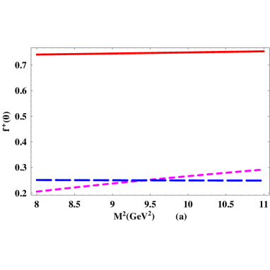
Figure 1: Left figure: The dependence form factor $f_{D_{s}}^{+}(0)$ on the Borel mass $M^{2}$(red solid line), the contribution of higher states in the whole sum rules(magenta short dashing line) and the contributions of the twist-3 light cone distribution amplitude’s contribution(blue long dashing line); Right figure: The dependence of form factor $f_{D_{s}}^{+}(q^{2})$ on the momentum transfer $q^{2}$ within the whole kinematical region.

Now, we can investigate the $q^{2}$ dependence of the form factors $f^{i}_{D_{s}}(q^{2})$ and $f^{i}_{D^{\ast}_{s0}}(q^{2})$. It is known that the OPE for the correlation function (24, 36) is valid only at small momentum transfer region $0<q^{2}<(m_{b}-m_{c})^{2}-2\Lambda_{\rm{QCD}}(m_{b}-m_{c})$. As for the case with the large momentum transfer (small recoil region), it is expected that HQET works well for the $b\to c$ transition. In the framework of HQET, the matrix elements responsible for $\bar{B}_{s}\to D_{sx}$ transition can be parameterized as Kurimoto:2002sb

$$\langle D^{*+}_{s0}(P)|\bar{c}\gamma_{\mu}\gamma_{5}b|\bar{B}_{s}(P+q)\rangle = -i\sqrt{m_{B_{s}}m_{D^{*}_{s0}}}[\eta_{D^{*}_{s0}}^{+}(w)(v+v^{\prime})_{\mu}+\eta_{D^{*}_{s0}}^{-}(w)(v-v^{\prime})_{\mu}],$$

$$\langle D^{+}_{s}(P)|\bar{c}\gamma_{\mu}b|\bar{B}_{s}(P+q)\rangle = \sqrt{m_{B_{s}}m_{D_{s}}}[\eta_{D_{s}}^{+}(w)(v+v^{\prime})_{\mu}+\eta_{D_{s}}^{-}(w)(v-v^{\prime})_{\mu}],$$ (43)

where $v=(P+q)/m_{B_{s}}$ and $v^{\prime}=P/m_{D_{sx}}$ are the four-velocity vectors of $B_{s}$ and $D_{sx}$ mesons with $D_{sx}$ being either $D_{s}$ or $D^{*}_{s0}$ meson and $w=v\cdot v^{\prime}$, Combining Eqs. (23), (36) and (43), we have

$$f_{i}^{+}(q^{2}) = \frac{1}{\sqrt{m_{B_{s}}m_{D_{sx}}}}[(m_{B_{s}}+m_{D_{sx}})\eta_{i}^{+}(w)-(m_{B_{s}}-m_{D_{sx}})\eta_{i}^{-}(w)],$$

$$f_{i}^{-}(q^{2}) = \sqrt{\frac{m_{D_{sx}}}{m_{B_{s}}}}[\eta_{i}^{+}(w)+\eta_{i}^{-}(w)],$$ (44)

with $w=(m_{B_{s}}^{2}+m_{D_{sx}}^{2}-q^{2})/2m_{B_{s}}m_{D_{sx}}$. In the heavy quark limit, the form factors $\eta_{D_{s}}^{+}(w)$ and $\eta_{D_{s}}^{-}(w)$ satisfy the following relations

$$\eta_{D_{s}}^{+}(w)=\xi(w),\qquad\eta_{D_{s}}^{-}(w)=0,$$ (45)

where $\xi(w)$ is the Isgur-Wise functionIsgur:1989vq ; Isgur:1989ed with the normalization $\xi(1)=1$. Similarly, heavy quark symmetry allows to relate the form factors $\eta_{D^{*}_{s0}}^{+}(w)$ and $\eta_{D^{*}_{s0}}^{-}(w)$ to a universal function $\tau_{1/2}(w)$Isgur:1990jf

$$\eta_{D^{*}_{s0}}^{+}(w)+\eta_{D^{*}_{s0}}^{-}(w)=-2\tau_{1/2}(w),\qquad\eta_{D^{*}_{s0}}^{+}(w)-\eta_{D^{*}_{s0}}^{-}(w)=2\tau_{1/2}(w).$$ (46)

An important relation between the $B\to D^{\ast\ast}$ form factors at zero recoil region and the slope $\rho^{2}$ of the $B\to D^{(\ast)}$ Isgur-Wise function is

$$\rho^{2}={1\over 4}+\sum_{n}|\tau_{1/2}^{(n)}|^{2}+\sum_{m}|\tau_{3/2}^{(m)}|^{2}$$ (47)

under the name of the Bjorken sum rule Isgur:1990jf . Here, $D^{\ast\ast}$ denotes the generic $L=1$ charmed states, the subscript $n$, $m$ identify the radial excitations of the states with the same $J^{P}$. For the $B\to D^{\ast\ast}$ transition form factors, the essential difference with the Isgur-Wise function $\xi(y)$ is that one can not invoke heavy quark symmetry arguments to predict the normalization of $\tau_{1/2}(w)$ DeFazio:2000up .

Phenomenologically, one can parameterize the $B_{s}\to D_{s}(1968,2317)$ form factors in the small recoil region as

$$\eta_{i}^{\pm}(w) = \eta_{i}^{\pm}(1)+a_{i}^{\pm}(w-1)+b_{i}^{\pm}(w-1)^{2},$$ (48)

where the $\eta_{i}^{\pm}(w)$ denotes the form factor $\eta_{D_{s}}^{\pm}(w)$ and $\eta_{D^{*}_{s0}}^{\pm}(w)$. The parameters $\eta_{i}^{\pm}(1)$, $a_{i}^{\pm}$ and $b_{i}^{\pm}$ can be determined under the condition that the form factors derived in the LCSR and HQET approaches should be connected in the vicinity of region with $q^{2}\sim(m_{b}-m_{c})^{2}-2\Lambda_{\rm{QCD}}(m_{b}-m_{c})$. In this way, we can derive the results of form factors in the whole kinematical region as shown in Fig. (1) as an example. The values of all form factors are tabulated in Table 1, where the results under the QCDSR approaches are also collected for comparison.

As can be observed from Table 1, the number of form factor $\eta_{D^{*}_{s0}}^{+}(w)$ at the zero-recoil region deviates from the zero significantly indicating that the $1/m_{c}$ power correction is sizeable for the $B\to D^{*}_{s0}$ transition. Generally, the expansion of the current

$$\bar{c}\Gamma_{i}b=\bar{c}_{v_{2}}\Gamma_{i}b_{v_{1}}-{1\over 2m_{c}}\bar{c}_{v_{2}}\Gamma_{i}i\!\!\not D_{2}b_{v_{1}}+{1\over 2m_{b}}\bar{c}_{v_{2}}\Gamma_{i}i\!\!\not D_{1}b_{v_{1}}+...$$ (49)

constitutes the main source of the power corrections. The QCDSR estimation of the form factor $f^{-}_{D^{*}_{s0}}$ differs from that obtained in the LCSR approach in sign implying that the power corrections and radiative corrections of correlation function are in need to reconcile the existing discrepancy between these two methods.

Table 1: Numbers of $f_{i}^{\pm}(0)$ and $\eta_{i}^{\pm}(w)$ determined from the LCSR approach, where the uncertainties from the Borel mass, threshold value, quark masses and decay constants are combined together. For comparison, the results estimated in the QCDSR are also collected here.

	this work	QCDSR	$\eta_{i}^{\pm}(1)$	$a_{i}^{\pm}$	$b_{i}^{\pm}$
$f_{D_{s0}}^{+}(q^{2})$	$0.53_{-0.11}^{+0.12}$	$0.40\pm 0.10$ Aliev:2006qy	$\eta_{D_{s0}}^{+}(w)$	$0.45_{-0.10}^{+0.11}$	$-0.79_{-0.20}^{+0.18}$	$0.92_{-0.20}^{+0.22}$
$f_{D_{s0}}^{-}(q^{2})$	$0.18_{-0.04}^{+0.06}$	$-0.12\pm 0.13$ Aliev:2006qy	$\eta_{D_{s0}}^{-}(w)$	$0.05_{-0.02}^{+0.02}$	$-0.12_{-0.05}^{+0.04}$	$0.17_{-0.05}^{+0.06}$
$f_{D_{s}}^{+}(q^{2})$	$0.86_{-0.15}^{+0.17}$	$0.70$Azizi:2008ty	$\eta_{D_{s}}^{+}(w)$	$0.79_{-0.14}^{+0.16}$	$-1.12_{-0.23}^{+0.20}$	$0.86_{-0.14}^{+0.16}$
$f_{D_{s}}^{-}(q^{2})$	$0.26_{-0.05}^{+0.06}$	$0.19$Azizi:2008ty	$\eta_{D_{s}}^{-}(w)$	$0.09_{-0.03}^{+0.03}$	$-0.16_{-0.03}^{+0.04}$	$0.14_{-0.03}^{+0.04}$

V Semileptonic and nonleptonic decays of $\bar{B}_{s}\to D_{s}(1968,2317)$

With the form factors derived above, we can further investigate the semileptonic and nonleptonic decays of $\bar{B}_{s}$ to $D_{s}(1968,2317)$ in the factorization approach. Factorization theorem is a basic theoretical tool to disentangle physical effects from different energy scales. Factorization in heavy quark decays was firstly proposed in Ref. Fakirov:1977ta as a phenomenological approximation similar to the vacuum saturation approximation for the four-quark operator matrix elements. Intuitively, factorization might work at least to leading-order approximation, since the partons that eventually form the emitted meson escape from the heavy meson remnant as an energetic, low mass, color singlet system, therefore independently from the remnant.

V.1 Semileptonic decays of $\bar{B}_{s}^{0}\to D_{s}^{+}(1968,2317)l\bar{\nu}_{l}$

With the free quark amplitude given above and the transition form factors derived in the LCSR, we arrive at the differential decay width for $\bar{B}_{s}^{0}\to D_{s}^{+}(1968,2317)l\bar{\nu}_{l}$ modes

$$\frac{d\Gamma}{dq^{2}} = \frac{G_{F}^{2}|V_{cb}|^{2}}{768\pi^{3}m_{B}^{3}}\frac{(q^{2}-m_{l}^{2})^{2}}{(q^{2})^{3}}\sqrt{\lambda}\bigg{[}\big{(}2m_{l}^{2}(\lambda+3q^{2}m_{Dx}^{2})+q^{2}\lambda\big{)}|f_{i}^{+}(q^{2})|^{2}$$ (50)

$$+6q^{2}m_{l}^{2}(m_{B}^{2}-m_{Dx}^{2}-q^{2})f_{i}^{+}(q^{2})f_{i}^{-}(q^{2})+6q^{4}m_{l}^{2}|f_{i}^{-}(q^{2})|^{2}\bigg{]},$$

with $\lambda=(m_{B}^{2}-m_{Dx}^{2}-q^{2})^{2}-4q^{2}m_{Dx}^{2}$.

Figure 2: The $q^{2}$ dependence of differential decay width $\frac{d}{dq^{2}}\Gamma(\bar{B}_{s}^{0}\to D_{s0}^{+}l^{-}\bar{\nu}_{l})$ for the final states with $l=e,\mu$ (left figure) and $l=\tau$ (right figure).

Figure 3: The $q^{2}$ dependence of differential decay width $\frac{d}{dq^{2}}\Gamma(\bar{B}_{s}^{0}\to D_{s}^{+}l^{-}\bar{\nu}_{l})$ for the final states with $l=e,\mu$ (left figure) and $l=\tau$ (right figure).

For convenience, the $q^{2}$ dependence of these invariant functions are also plotted in Fig. 2 and 3. Integrating Eq. (50), we get the branching fractions of $\bar{B}_{s}^{0}\to D_{s}^{+}(1968,2317)l\bar{\nu}_{l}$ as grouped in Table 2. It can be observed from this table that the orders of magnitudes for $BR(\bar{B}_{s}^{0}\to D_{s}^{+}(1968,2317)l\bar{\nu}_{l})$ obtained in the quark model and sum rule approaches are consistent with each other. Besides, we can also find that the decay rates for the final state with $\tau$ lepton are generally $3-4$ times smaller than those for the muon case due to the suppression of phase spaces. Once the data on the $\bar{B}_{s}^{0}\to D_{s}^{+}(2317)l\bar{\nu}_{l}$ are available, the theoretical predictions presented here can be put to the experimental scrutiny to test the ordinary $c\bar{s}$ picture of $D_{s}(2317)$ meson.

Table 2: Branching ratios for the semileptonic decays $\bar{B}_{s}^{0}\to D_{s}^{+}(1968,2317)l\bar{\nu}_{l}$ with the form factors estimated in LCSR, where the results calculated in constituent quark model and QCDSR are also displayed for comparison.

$\bar{B}_{s}^{0}\to D_{s0}^{+}l^{-}\bar{\nu}_{l}$	$l=e,\mu$	$l=\tau$
this work	$(2.3_{-1.0}^{+1.2})\times 10^{-3}$	$(5.7_{-2.3}^{+2.8})\times 10^{-4}$
QCDSRAliev:2006qy	$\sim 10^{-3}$	$\sim 10^{-4}$
Constituent Quark ModelZhao:2006at	$(4.90-5.71)\times 10^{-3}$
QCDSR in HQETHuang:2004et	$(0.9-2.0)\times 10^{-3}$
$\bar{B}_{s}^{0}\to D_{s}^{+}l^{-}\bar{\nu}_{l}$	$l=e,\mu$	$l=\tau$
this work	$(1.0_{-0.3}^{+0.4})\times 10^{-2}$	$(3.3_{-1.1}^{+1.4})\times 10^{-3}$
Constituent Quark ModelZhao:2006at	$(2.73-3.00)\times 10^{-2}$
QCDSR Azizi:2008tt	$(2.8-3.8)\times 10^{-2}$

V.2 Nonleptonic decays of $\bar{B}_{s}\to D_{s}^{+}(1968,2317)M$

Now, we turn to the calculations of nonleptonic decays $\bar{B}_{s}\to D_{s}^{+}(1968,2317)M$, where $M$ can be a light meson or a charmed meson. As mentioned above, the factorization assumption will be employed to decompose the matrix element of four-quark operator

$$\langle D_{sx}M|Q|\bar{B}_{s}\rangle=\langle M|j_{2}|0\rangle\langle D_{sx}|j_{1}|\bar{B}_{s}\rangle,$$ (51)

into the the $\bar{B}_{s}\to D_{s}^{+}(1968,2317)$ transition form factors and the decay constant of $M$.

For a light meson $M$, only the tree-operators in Eq. (2) can contribute to these decay modes induced by the $b\to c$ transition. Then, the decay width for $\bar{B}_{s}\to D_{s}^{+}(1968,2317)L$ can be written as

$$\Gamma(\bar{B}_{s}\to D_{sx}^{+}L^{-}) = \frac{G_{F}^{2}|\vec{P}|}{16\pi m^{2}_{B_{s}}}|V_{cb}V^{*}_{uq}a_{2}(\mu)|^{2}f_{L}^{2}\times\bigg{\{}\begin{array}[]{cc}|f_{D_{sx}}^{+}(m^{2}_{L})m_{L}(\epsilon^{*}\cdot P)|^{2}\hskip 85.35826pt(\mbox{$L$=$V$}),\\ |\frac{m^{2}_{B_{s}}-m^{2}_{D_{sx}}-m^{2}_{L}}{2}f_{D_{sx}}^{+}(m^{2}_{L})+f_{D_{sx}}^{-}(m^{2}_{L})m^{2}_{L}|^{2}\;\;\hskip 5.69046pt(\mbox{$L$=$S,\,\,P$}),\end{array}$$ (54)

where $L$ denotes a light meson; $V$, $P$ and $S$ label the vector, pseudoscalar and scalar mesons respectively. The magnitude of the three-momentum for the recoiled charmed meson is

$$|\vec{P}|=\frac{[(m^{2}_{B_{s}}-(m_{D_{sx}}+m_{L})^{2})(m^{2}_{B_{s}}-(m_{D_{sx}}-m_{L})^{2})]^{1/2}}{2m_{B_{s}}},$$ (55)

and the decay constant $f_{L}$ has been collected in Table 3. The decay constants for the light pseudoscalar mesons are taken from the Particle Data Group pdg and the vector meson longitudinal decay constants are extracted from the data on $\tau^{-}\to(\rho^{-},K^{*-})\nu_{\tau}$. To determine the decay constants for the scalar meson $D_{0}^{\ast}$ and vector meson $D_{s}^{\ast}$, the following relation

$${f_{D_{s0}^{\ast}}\over f_{D_{0}^{\ast}}}\approx{f_{D_{s}^{\ast}}\over f_{D^{\ast}}}\approx{f_{B_{s}}\over f_{B}}$$ (56)

is assumed in this work. The decay constant of vector meson $D^{\ast}$ is borrowed from Ref. Colangelo:2000dp . The energy scale of the Wilson coefficient $a_{2}(\mu)$ is varied from $0.5m_{b}$ to $1.5m_{b}$ in the error estimations.

Table 3: Decay constants of light and charmed mesons (unit: $\rm{MeV}$).

$f_{\pi}$	$f_{K}$	$f_{\rho}$	$f_{K^{*}}$	$f_{D}$	$f_{D_{0}^{*}}$	$f_{D^{*}}$	$f_{D_{s}^{*}}$
$131$	$160$	$209\pm 2$	$217\pm 5$	$206\pm 9$	$95\pm 10$	$270\pm 35$	$312\pm 40$

Substituting the form factors obtained in the previous sections into Eq. (54), we can get the decay rates of $\bar{B}_{s}\to D_{s}^{+}(1968,2317)L$ as shown in Table 4. From this table, the results evaluated in the factorization approach are in accord with that predicted in the PQCD approach and the available data, which implies that the factorization assumption (FA) works well for these color allowed modes as expected.

Table 4: Branching ratios(unit: $10^{-4}$) for the nonleptonic decays $\bar{B}_{s}\to D_{sx}^{+}L$ ($L$ denotes a light meson) estimated in the FA with the form factors obtained in the LCSR, where we have combined the uncertainties from the form factors, the scale-dependence and CKM matrix elements. In Ref. Azizi:2008ty , the authors also employ the naive factorization but take the transition form factors calculated in the three-point sum rules.

Channels	this work	PQCDLi:2008ts	Exp.pdg	FA Azizi:2008ty
$\bar{B}_{s}^{0}\to D^{\ast+}_{s0}\pi^{-}$	$5.2_{-2.1}^{+2.5}$
$\bar{B}_{s}^{0}\to D^{\ast+}_{s0}K^{-}$	$0.4_{-0.2}^{+0.2}$
$\bar{B}_{s}^{0}\to D^{\ast+}_{s0}\rho^{-}$	$13_{-5}^{+6}$
$\bar{B}_{s}^{0}\to D^{\ast+}_{s0}K^{*-}$	$0.8_{-0.3}^{+0.4}$
$\bar{B}_{s}^{0}\to D^{+}_{s}\pi^{-}$	$17_{-6}^{+7}$	$19.6_{-7.5-6.2-0.6}^{+10.6+6.3+0.6}$	$32\pm 9$	$11.2\pm 22.7$
$\bar{B}_{s}^{0}\to D^{+}_{s}K^{-}$	$1.3_{-0.4}^{+0.5}$	$1.70_{-0.66-0.56-0.05}^{+0.87+0.53+0.05}$		$0.83\pm 2.51$
$\bar{B}_{s}^{0}\to D^{+}_{s}\rho^{-}$	$42_{-14}^{+17}$	$47.0_{-17.7-14.8-1.37}^{+24.9+15.3+1.36}$
$\bar{B}_{s}^{0}\to D^{+}_{s}K^{*-}$	$2.4_{-0.8}^{+1.0}$	$2.81_{-1.09-0.85-0.09}^{+1.47+0.79+0.09}$		$0.60\pm 2.82$

Moreover, it is also helpful to define the following ratios

$$R_{1} \equiv {BR(\bar{B}_{s}^{0}\to D^{\ast+}_{s0}\pi^{-})\over BR(\bar{B}_{s}^{0}\to D^{\ast+}_{s0}K^{-})}\approx{BR(\bar{B}_{s}^{0}\to D^{+}_{s}\pi^{-})\over BR(\bar{B}_{s}^{0}\to D^{+}_{s}K^{-})}\approx\bigg{|}{V_{ud}\over V_{us}}{f_{\pi}\over f_{K}}\bigg{|}^{2}\approx 12.6,$$

$$R_{2} \equiv {BR(\bar{B}_{s}^{0}\to D^{\ast+}_{s0}\rho^{-})\over BR(\bar{B}_{s}^{0}\to D^{\ast+}_{s0}K^{*-})}\approx{BR(\bar{B}_{s}^{0}\to D^{+}_{s}\rho^{-})\over BR(\bar{B}_{s}^{0}\to D^{+}_{s}K^{*-})}\approx\bigg{|}{V_{ud}\over V_{us}}{f_{\rho}\over f_{K^{\ast}}}\bigg{|}^{2}\approx 17.4,$$ (57)

which are consistent with those collected in Table 4.

As for the two charmed meson decays of $B_{s}$ meson, the decay width in the factorization approach can be given by

$$\Gamma(\bar{B}_{s}\to D_{sx}^{+}X) = \frac{G_{F}^{2}|\vec{P}|}{16\pi m^{2}_{B_{s}}}|V_{cb}V^{*}_{cq}a_{2}(\mu)-V_{tb}V^{*}_{tq}[a_{4}(\mu)+a_{10}(\mu)+r_{q}(a_{6}(\mu)+a_{8}(\mu))]|^{2}f_{X}^{2}$$ (60)

$$\times\bigg{\{}\begin{array}[]{cc}|f_{D_{sx}}^{+}(m^{2}_{X})m_{X}(\epsilon^{*}\cdot P)|^{2}\hskip 108.12054pt(\mbox{$X$=$V$}),\\ |\frac{m^{2}_{B_{s}}-m^{2}_{D_{sx}}-m^{2}_{X}}{2}f_{D_{sx}}^{+}(m^{2}_{X})+f_{D_{sx}}^{-}(m^{2}_{X})m^{2}_{X}|^{2}\;\;\hskip 28.45274pt(\mbox{$X$=$S,\,\,P$}),\end{array}$$

with

$$r_{q}=\left\{\begin{array}[]{rrrrr}{2m_{X}^{2}\over(m_{b}-m_{c})(m_{c}+m_{q})}\hskip 28.45274pt(\bar{B}_{s}^{0}\to D_{s}^{+}X,\;\mbox{$X$=$P$}),\\ {2m_{X}^{2}\over(m_{b}-m_{c})(m_{c}-m_{q})}\hskip 28.45274pt(\bar{B}_{s}^{0}\to D_{s}^{+}X,\;\mbox{$X$=$S$}),\\ -{2m_{X}^{2}\over(m_{b}-m_{c})(m_{c}-m_{q})}\hskip 28.45274pt(\bar{B}_{s}^{0}\to D_{s0}^{*+}X,\;\mbox{$X$=$P$}),\\ -{2m_{X}^{2}\over(m_{b}-m_{c})(m_{c}-m_{q})}\hskip 28.45274pt(\bar{B}_{s}^{0}\to D_{s0}^{*+}X,\;\mbox{$X$=$S$}),\\ 0\hskip 71.13188pt(\bar{B}_{s}^{0}\to D_{sx}^{+}X,\;\mbox{$X$=$V$}),\\ \end{array}\right\}$$ (66)

where the quark masses in the above equation are the current quark masses.

Combining the Eq. (60) and the form factors listed above, one can easily get the branching ratios of $\bar{B}_{s}\to D_{sx}^{+}X$ ($X$ being a charmed meson) as shown in Table 5. As can be seen from this table, the decay model $\bar{B}_{s}^{0}\to D^{+}_{s0}D_{s}^{-}$ possesses a quite large branching ratio of order $10^{-2}$, which should be detected easily at the large colliders such as Tevatron and LHC. Moreover, the theoretical predictions on the $\bar{B}_{s}^{0}\to D^{+}_{s}\pi^{-}$ decay can accommodate the experimental data within the error bars. As for the $\bar{B}_{s}^{0}\to D^{+}_{s}D_{s}^{*-}$ decay, only the upper bound for this mode is available at present, which is also respected by our predictions.

Subsequently, the ratio of decay rates between the Cabibbo favored and suppressed modes can be estimated as

$$R_{3} \equiv {BR(\bar{B}_{s}^{0}\to D^{\ast+}_{s0}D_{s}^{-})\over BR(\bar{B}_{s}^{0}\to D^{\ast+}_{s0}D^{-})}\approx{BR(\bar{B}_{s}^{0}\to D^{+}_{s}D_{s}^{-})\over BR(\bar{B}_{s}^{0}\to D^{+}_{s}D^{-})}\approx\bigg{|}{V_{cs}\over V_{cd}}{f_{D_{s}^{-}}\over f_{D^{-}}}\bigg{|}^{2},$$

$$R_{4} \equiv {BR(\bar{B}_{s}^{0}\to D^{\ast+}_{s0}D_{s}^{\ast-})\over BR(\bar{B}_{s}^{0}\to D^{\ast+}_{s0}D^{\ast-})}\approx{BR(\bar{B}_{s}^{0}\to D^{+}_{s}D_{s}^{\ast-})\over BR(\bar{B}_{s}^{0}\to D^{+}_{s}D^{\ast-})}\approx\bigg{|}{V_{cs}\over V_{cd}}{f_{D_{s}^{\ast-}}\over f_{D^{\ast-}}}\bigg{|}^{2},$$

$$R_{5} \equiv {BR(\bar{B}_{s}^{0}\to D^{\ast+}_{s0}D_{s0}^{\ast-})\over BR(\bar{B}_{s}^{0}\to D^{\ast+}_{s0}D_{0}^{*-})}\approx{BR(\bar{B}_{s}^{0}\to D^{+}_{s}D_{s0}^{\ast-})\over BR(\bar{B}_{s}^{0}\to D^{+}_{s}D_{0}^{*-})}\approx\bigg{|}{V_{cs}\over V_{cd}}{f_{D_{s0}^{\ast-}}\over f_{D_{0}^{\ast-}}}\bigg{|}^{2},$$ (67)

in the naive factorization without the contributions from penguin operators. Such naive estimations are in good agreement with that presented in Table 5, which also indicates that the two charmed-meson decays of $B_{s}$ meson governed by the $b\to qc\bar{c}$ ($q=s\,\,d$) transition are dominated by the tree operators.

Table 5: Branching ratios(unit: $10^{-3}$) for the nonleptonic decays $\bar{B}_{s}\to D_{sx}^{+}X$ ($X$ denotes a charmed meson) estimated in the FA with the form factors obtained in the LCSR, where the uncertainties from the form factors, the scale-dependence and CKM matrix elements have been combined together.

Channels	This work	Exp. pdg
$\bar{B}_{s}^{0}\to D^{\ast+}_{s0}D_{s}^{-}$	$13_{-5}^{+7}$
$\bar{B}_{s}^{0}\to D^{\ast+}_{s0}D^{-}$	$0.5_{-0.2}^{+0.2}$
$\bar{B}_{s}^{0}\to D^{\ast+}_{s0}D_{s0}^{-}$	$2.1_{-0.8}^{+1.0}$
$\bar{B}_{s}^{0}\to D^{\ast+}_{s0}D_{0}^{*-}$	$0.2_{-0.1}^{+0.1}$
$\bar{B}_{s}^{0}\to D^{\ast+}_{s0}D_{s}^{*-}$	$6.0_{-2.4}^{+2.9}$
$\bar{B}_{s}^{0}\to D^{\ast+}_{s0}D^{*-}$	$0.2_{-0.1}^{+0.1}$
$\bar{B}_{s}^{0}\to D^{+}_{s}D_{s}^{-}$	$35_{-12}^{+14}$	$110\pm 40$
$\bar{B}_{s}^{0}\to D^{+}_{s}D^{-}$	$1.1_{-0.4}^{+0.4}$
$\bar{B}_{s}^{0}\to D^{+}_{s}D_{s0}^{\ast-}$	$5.3_{-1.8}^{+2.2}$
$\bar{B}_{s}^{0}\to D^{+}_{s}D_{0}^{*-}$	$0.2_{-0.1}^{+0.1}$
$\bar{B}_{s}^{0}\to D^{+}_{s}D_{s}^{*-}$	$33_{-11}^{+13}$	$<121$
$\bar{B}_{s}^{0}\to D^{+}_{s}D^{*-}$	$1.4_{-0.5}^{+0.6}$

VI Discussion and conclusion

A detailed analysis of properties about the new charming mesons such as $D_{s}(2317)$ has become a prominent part of the ongoing and forthcoming experimental programs at various facilities worldwide. The production characters of charmed mesons in the $B_{s}$ decays are especially interesting for highlighting the understanding of QCD dynamics and enriching our knowledge of flavor physics. More importantly, the theory underlying the description of the decays induced by the $b\to c$ transition is mature currently. In view of the large mass of $b$ quark, heavy quark expansion works well enough to enable a precise determination of the decay amplitude.

LCSR approach is employed to compute the $\bar{B}_{s}^{0}\to D_{s}^{+}(1968,2317)$ transition form factors at the large recoil region and the results are then extended to the small recoil region in the framework of HQET. Our results show that the power correction to the form factor $\eta_{D_{s}}^{+}(w)$ responsible for the $\bar{B}_{s}^{0}\to D_{s}^{+}(1968)$ at the zero-recoil region transition is numerically small, since this form factor only receive the corrections at order $1/m_{b}^{2}$ and $1/m_{c}^{2}$ as indicated by the Luke’s theorem Luke . However, the power correction to the form factor $\eta_{D_{s0}^{\ast}}^{+}(w)$ relevant to the $B\to D_{s0}^{\ast+}$ transition is sizeable.

Subsequently, we utilize the form factors estimated in the LCSR approach to perform a careful study on the semileptonic decays $\bar{B}_{s}^{0}\to D_{s}^{+}(1968,2317)l\bar{\nu}_{l}$. It has been shown in this work that the branching fraction of the semileptonic $\bar{B}_{s}^{0}\to D_{s}^{+}(2317)\mu\bar{\nu}_{\mu}$ decay is around $2.3\times 10^{-3}$, which should be detectable with ease at the Tevatron and LHC. The decay rates of semileptonic modes for the final states with $\tau$ lepton are approximately $3-4$ times smaller than those with muon due to the suppression of phase spaces. In addition, the branching fractions of $\bar{B}_{s}^{0}\to D_{s}^{+}(1968)l\bar{\nu}_{l}$ are almost one order large than that for the $B_{s}^{0}\to D_{s}^{+}(2317)l\bar{\nu}_{l}$ decays.

Nonleptonic decays $B_{s}\to D_{s}^{+}(1968,2317)M$ are also investigated in the framework of factorization approach in this work. It is found that the theoretical predictions for $B_{s}\to D_{s}^{+}(1968,2317)L$ presented here are in agreement with those obtained in the $k_{T}$ factorization, which supports the success of color transparence mechanism in the color allowed decay modes. Moreover, $\bar{B}_{s}^{0}\to D^{\ast+}_{s0}D_{s}^{-}$ owns a quite large branching ratio as $1.3\times 10^{-2}$, which should be accessible experimentally. More theoretical results worked out here are expected to be tested by the large colliders in the near future.

References

• (1) B. Aubert et al. [BABAR Collaboration], Phys. Rev. Lett.  90, 242001 (2003) [arXiv:hep-ex/0304021].
• (2) For a review, see F. De Fazio, arXiv:hep-ph/0010007.
• (3) S. M. Zhao, X. Liu and S. J. Li, Eur. Phys. J.  C 51, 601 (2007) [arXiv:hep-ph/0612008].
• (4) M. Q. Huang, Phys. Rev.  D 69, 114015 (2004) [arXiv:hep-ph/0404032].
• (5) T. M. Aliev and M. Savci, Phys. Rev.  D 73, 114010 (2006) [arXiv:hep-ph/0604002].
• (6) K. Azizi, Nucl. Phys.  B 801, 70 (2008) [arXiv:0805.2802 [hep-ph]].
• (7) R. H. Li, C. D. Lu and H. Zou, Phys. Rev.  D 78, 014018 (2008) [arXiv:0803.1073 [hep-ph]].
• (8) S. Hashimoto, A. X. El-Khadra, A. S. Kronfeld, P. B. Mackenzie, S. M. Ryan and J. N. Simone, Phys. Rev.  D 61, 014502 (1999) [arXiv:hep-ph/9906376].
• (9) G. M. de Divitiis, E. Molinaro, R. Petronzio and N. Tantalo, Phys. Lett.  B 655, 45 (2007) [arXiv:0707.0582 [hep-lat]].
• (10) G. M. de Divitiis, R. Petronzio and N. Tantalo, JHEP 0710, 062 (2007) [arXiv:0707.0587 [hep-lat]].
• (11) I. I. Balitsky, V. M. Braun and A. V. Kolesnichenko, Nucl. Phys.  B 312 (1989) 509.
• (12) I. I. Balitsky, V. M. Braun and A. V. Kolesnichenko, Sov. J. Nucl. Phys.  44 (1986) 1028 [Yad. Fiz.  44 (1986) 1582].
• (13) V. M. Braun and I. E. Filyanov, Z. Phys.  C 44 (1989) 157 [Sov. J. Nucl. Phys.  50 (1989 YAFIA,50,818-830.1989) 511.1989 YAFIA,50,818].
• (14) V. L. Chernyak and I. R. Zhitnitsky, Nucl. Phys.  B 345 (1990) 137.
• (15) P. Ball, V. M. Braun and H. G. Dosch, Phys. Rev.  D 44 (1991) 3567.
• (16) M. A. Shifman, A. I. Vainshtein and V. I. Zakharov, Nucl. Phys.  B 147 (1979) 385.
• (17) M. A. Shifman, A. I. Vainshtein and V. I. Zakharov, Nucl. Phys.  B 147 (1979) 519.
• (18) M. A. Shifman, A. I. Vainshtein and V. I. Zakharov, Nucl. Phys.  B 147 (1979) 448.
• (19) V. M. Braun, Plenary talk given at the IVth International Workshop on Progress in Heavy Quark Physics Rostock, Germany, 20–22 September 1997, arXiv:hep-ph/9801222.
• (20) P. Ball, V.M. Braun, Phys. Rev. D 55, 5561 (1997) [arXiv:hep-ph/9701238].
• (21) P. Ball, J. High Energy Phys. 9809, 005 (1998) [arXiv:hep-ph/9802394].
• (22) A. Khodjamirian, R. Ruckl, S. Weinzierl, C.W. Winhart, O.I. Yakovlev, Phys. Rev. D 62, 114002 (2000) [arXiv:hep-ph/0001297].
• (23) P. Ball, R. Zwicky, Phys. Rev. D 71, 014015 (2005) [arXiv:hep-ph/0406232].
• (24) B. Melic, Phys. Lett. B 591, 91 (2004) [arXiv:hep-ph/0404003].
• (25) Y.M. Wang, C.D. Lü, Phys. Rev. D 77, 054003 (2008) [arXiv:0707.4439 [hep-ph]].
• (26) Y. M. Wang, M. J. Aslam and C. D. Lu, Phys. Rev.  D 78, 014006 (2008) [arXiv:0804.2204 [hep-ph]].
• (27) M.Q. Huang, D.W. Wang, Phys. Rev. D 69, 094003 (2004) [arXiv:hep-ph/0401094].
• (28) Y. M. Wang, Y. Li and C. D. Lü, Eur. Phys. J.  C 59, 861 (2009) [arXiv:0804.0648 [hep-ph]].
• (29) A. Ali, G. Kramer, and C. -D. Lü, Phys. Rev. D58, 094009 (1998) [arXiv:hep-ph/9804363]; Phys. Rev. D59, 014005 (1999) [arXiv:hep-ph/9805403]; Y. H. Chen, H. Y. Cheng, B. Tseng, and K. C. Yang, Phys. Rev. D60, 094014 (1999) [arXiv:hep-ph/9903453].
• (30) T. Kurimoto, H. n. Li and A. I. Sanda, Phys. Rev.  D 67, 054028 (2003) [arXiv:hep-ph/0210289].
• (31) C. H. Chen, Phys. Rev.  D 68, 114008 (2003) [arXiv:hep-ph/0310290].
• (32) P. Colangelo, F. De Fazio and A. Ozpineci, Phys. Rev.  D 72, 074004 (2005) [arXiv:hep-ph/0505195].
• (33) I.I. Balitsky and V.M. Braun, Nucl. Phys. B311,541(1989).
• (34) A. Khodjamirian and R. Ruckl, Adv. Ser. Direct. High Energy Phys.  15 (1998) 345 [arXiv:hep-ph/9801443].
• (35) M. Diehl, T. Feldmann, R. Jakob and P. Kroll, Eur. Phys. J.  C 8 (1999) 409 [arXiv:hep-ph/9811253]
• (36) C. Amsler et al. (Particle Data Group), Phys. Lett. B667, 1 (2008).
• (37) J. Charles et al. (The CKMfitter Group); Eur. Phys. J. C41, 1 (2005) [hep-ph/0406184]. The input values for the CKM parameters are taken from the unitarity fits reported on March 7, 2009 (http://ckmfitter.in2p3.fr/).
• (38) T. M. Aliev and V. L. Eletsky, Sov. J. Nucl. Phys.  38, 936 (1983) [Yad. Fiz.  38, 1537 (1983)].
• (39) P. Colangelo and A. Khodjamirian, arXiv:hep-ph/0010175.
• (40) B.L. Ioffe, Prog. Part. Nucl. Phys. 56, 232 (2006) [arXiv:hep-ph/0502148].
• (41) H.G. Dosch, E.M. Ferreira, F.S. Navarra and M. Nielsen, Phys. Rev. D 65 (2002) 114002 [arXiv:hep-ph/0203225].
• (42) R.D. Matheus, F.S. Navarra, M. Nielsen and R. Rodrigues da Silva, Phys. Lett. B 541 (2002) 265 [arXiv:hep-ph/0206198].
• (43) M.E. Bracco, M. Chiapparini, F.S. Navarra and M. Nielsen, Phys. Lett. B 605 (2005) 326 [arXiv:hep-ph/0410071].
• (44) F.S. Navarra, Marina Nielsen, M.E. Bracco, M. Chiapparini and C.L. Schat, Phys. Lett. B 489 (2000) 319 [arXiv:hep-ph/0005026].
• (45) Y. M. Wang, H. Zou, Z. T. Wei, X. Q. Li and C. D. Lu, Eur. Phys. J.  C 54 (2008) 107 [arXiv:0707.1138 [hep-ph]].
• (46) P. Colangelo, G. Nardulli and N. Paver, Z. Phys. C 57, 43 (1993).
• (47) N. Isgur and M. B. Wise, Phys. Lett.  B 232, 113 (1989).
• (48) N. Isgur and M. B. Wise, Phys. Lett.  B 237, 527 (1990).
• (49) N. Isgur and M. B. Wise, Phys. Rev.  D 43, 819 (1991).
• (50) K. Azizi, R. Khosravi and F. Falahati, arXiv:0811.2671 [hep-ph].
• (51) D. Fakirov and B. Stech, Nucl. Phys.  B 133 (1978) 315.
• (52) M.E. Luke, Phys. Lett.  B 252, 447 (1990).