Parent Hamiltonian for the Chiral Spin Liquid

Abstract

We present a method for constructing parent Hamiltonians for the chiral spin liquid. We find two distinct Hamiltonians for which the chiral spin liquid on a square lattice is an exact zero-energy ground state. We diagonalize both Hamiltonians numerically for 16-site lattices, and find that the chiral spin liquid, modulo its two-fold topological degeneracy, is indeed the unique ground state for one Hamiltonian, while it is not unique for the other.

I Introduction

The first notion of fractional excitations in condensed matter physics goes back to the appearance of soliton mid-gap modes in polyacetylene su-79prl1698 , where the effective net charge of one kink excitation is $e/2$, i.e., one half of the electron charge. At a similar time, the field of fractional statistics, founded in the work by Leinaas and Myrheim leinaas-77ncb1 , attained broad attention due to the work by Wilczek in 1982 wilczek82prl1144 ; wilczek82prl957 . In strongly-correlated many-body systems, the phenomenon of fractionalization, where the elementary excitations of the system carry only a fraction of the quantum numbers of the constituents, has become known to occur in a variety of cases.

The first physical system in which fractional excitations and the associated fractional statistics have been discussed on a unified footing is the fractional quantum Hall effect laughlin83prl1395 ; halperin84prl1583 ; arovas-84prl722 (FQHE). There, the quantum statistics of the anyonic quasiparticles can be understood in terms of a generalized Berry’s phase Wilczek90 , which is acquired by the wave function as quasiparticles wind around each other. This is a sensible concept in two dimensions only where one can uniquely define a winding number for the braiding. In the FQHE, the fractional statistics is known to occur in the presence of a magnetic field violating parity (P) and time-reversal (T) symmetry. In recent years, there have been tremendous efforts to study the fractional excitations of the FQHE experimentally in order to confirm the prediction from theory and to validate fractional statistics as a concept being realized in nature. This, however, has remained inconclusive in certain aspects and thus is still a subject of current discussion and work goldman-95s1010 ; depicciotto-97n162 ; reznikov-99n238 ; camino-05prl246802 ; feldman-07prb085333 .

Later, the concept of fractional statistics has been found to occur in one-dimensional spin-1/2 antiferromagnets, where it can be defined in terms of a generalized Pauli principle obeyed by the excitations haldane91prl937 and, as shown recently, by a phase the wave function acquires when two spinons move through each other greiter09prb064409 . The fractional charge of the quasiparticles in the FQHE corresponds to the spin $1/2$ of the elementary spinon excitations in these systems, which is fractional as the Hilbert space is built up by spin flips which carry spin $1$. As one-dimensional systems are amenable to a host of exact methods, many exactly solvable models exhibiting this behavior exist haldane88prl635 ; shastry88prl639 ; haldane91prl1529 ; haldane-92prl2021 . In particular, various properties of fractional excitations in spin chains have been observed experimentally tennant-93prl4003 ; coldea-97prl151 ; kim-06np397 .

In general, it appears to be that $\mathrm{P}$ and $\mathrm{T}$ violation is intimately related to the occurrence of excitations obeying fractional statistics in two dimensions, which both applies to quasiparticles in the FQHE and spinons in a quantum antiferromagnet. These symmetries may be explicitly broken as in the FQHE or generated by spontaneous symmetry breaking. For two-dimensional antiferromagnets, the concept of fractional excitations is less established than for the one-dimensional case nayak-01prb064422 . In particular, finding solvable theoretical models in which the phenomenon occurs has been one predominant area of research in the field. Significant progress has been accomplished for dimer models misguich-02prl137202 ; moessner-01prl1881 .

In addition to important questions with regard to the general principle underlying fractional statistics, two-dimensional spin liquids are of special interest with regard to investigation of the hypothesized link between fractionalization and high-$T_{\text{c}}$ superconductivity anderson87s1197 ; kivelson-87prb8865 . Moreover, in many systems where fractionalization occurs, there is the ambition to use the topological degeneracy contained in these systems for quantum computing, where topological information can serve as a quantum bit with negligibly small local decoherence rates Kitaev02ap2 .

The paradigmatic state for a $S=1/2$ spin liquid is the chiral spin liquid (CSL) introduced by Kalmeyer and Laughlin kalmeyer-87prl2095 ; kalmeyer-89prb11879 , which is constructed to spontaneously violate the symmetries $\mathrm{P}$ and $\mathrm{T}$, and can be defined on any regular lattice including both bipartite and non-bipartite lattices. The universality class of chiral spin liquid states, and in particular the order parameter and the topological degeneracy wen-89prb7387 , was defined by Wen, Wilczek, and Zee wen-89prb11413 . A CSL state has also been constructed by Yao and Kivelson yao-07prl247203 in the Kitaev model Kitaev06ap2 on a Fisher lattice, i.e., a honeycomb lattice of triangles. Recently, a family of non-Abelian CSL states greiter-09prl207203 has been proposed for general spin $S$, whose wave functions correspond to the bosonic Read-Rezayi series of FQH states Read-99prb8084 . The non-Abelian statistics of the spinons has even been conjectured to be a general property of spin $S$ antiferromagnets greiter-09prl207203 .

As in the one-dimensional case mentioned above, the spinons in the CSL exhibit quantum-number fractionalization and carry only half the spin of the bosonic spin excitations in conventional magnetically-ordered systems, which carry spin $1$. Whereas the spinon appears to be the fundamental field describing excitations in two-dimensional $S=1/2$ antiferromagnets in general, an effective description by magnon-like excitations proved rather adequate for the generic model. The reason for this is that the confinement between the spinons is generically so strong that the underlying excitation structure is mostly suppressed. In the CSL, however, the spinons are deconfined. The model is hence ideally suited to study fractional quantization of spinons in two-dimensional antiferromagnets. In spite of its promising properties, for nearly two decades since its emergence, the CSL lacked a microscopic model where it is realized.

In this article, we develop an analytical method for the construction of parent Hamiltonians for the CSL. The method relies explicitly on the singlet property of the CSL, as this allows for a spherical tensor decomposition of the destruction operator we introduce. From different tensor components, we construct two different parent Hamiltonians, which annihilate the CSL and hence have it as a zero-energy ground state. One of the Hamiltonians has been presented in a Letter previously schroeter-07prl097202 ; both Hamiltonians contain 6-body interactions. One of the key issues we address here is whether the CSL is the only ground state of these Hamiltonians. To answer this question, we perform exact diagonalization studies of both models for a 16-site square lattice. In particular, we introduce an adapted Kernel sweeping method, which allows for an efficient numerical implementation of the complex and technically cumbersome Hamiltonians we investigate. We find that the model we introduced previously has indeed the CSL as its (modulo the two-fold topological degeneracy) unique ground state. For the other Hamiltonian we present, however, we find that the CSL is not the unique ground state. Hence only the former model is useful for further analysis of e.g. the spinon spectrum.

The paper is organized as follows. In Section II, we review the chiral spin liquid ground state and its basic properties. After outlining the general construction scheme for the Hamiltonians in Section III, we formulate a destruction operator for the CSL state in Section IV and exploit the spin rotational invariance of the CSL state to decompose the destruction operator into its spherical tensor components, which annihilate the CSL state individually. The proof that the destruction operator annihilates the CSL ground state is given in Section V. In Section VI, we introduce a Kernel sweeping method to compute the CSL Hamiltonians. We present the method in detail and emphasize its applicability to efficiently compute $n$-body interactions for finite-size exact diagonalization studies. The numerical results obtained with this method are discussed in Section VII. We conclude this work with a summary in Section VIII.

II Chiral Spin Liquid

The CSL was originally conceived by D.H. Lee as a spin liquid constructed by condensing the bosonic spin flip operators on a two-dimensional lattice into a FQH liquid at Landau level filling factor $\nu=1/2$. The ground state wave function for a circular droplet with open boundary conditions, on a square lattice with lattice constant of length one, is given by kalmeyer-87prl2095 ; kalmeyer-89prb11879

$$\left\langle z_{1}\cdots z_{M}|\psi\right\rangle=\prod_{j<k}^{M}\,(z_{j}-z_{k})^{2}\;\prod_{j=1}^{M}\,G(z_{j})\,e^{-\frac{\pi}{2}|z_{j}|^{2}}\,,$$ (1)

where $M=N/2$. The $z$’s in the above expression are the complex positions of the up-spins on the lattice: $z=x+iy$, with $x$ and $y$ integer. $G(z)=(-1)^{(x+1)(y+1)}$ is a gauge factor, which ensures that (1) is a spin singlet (see Fig. 1). Lattice sites not occupied by $z$’s correspond to down-spins.

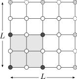
Figure 1: The model is defined on a square lattice length $L$ on a side such that the total number of sites is given by $N=L^{2}$. The image shows the lattice for $N=16$. The shaded circles (including the origin) indicate those lattice sites for which $G\!\left(z\right)=-1$ and the open circles those sites for which $G\!\left(z\right)=+1$. The sites on which $G\!\left(z\right)=-1$ define a sublattice with twice the original lattice spacing; the doubled unit-cell is shown as the shaded region in the figure surrounding the origin.

For our purposes, it is propitious to choose periodic boundary conditions (PBCs) with equal periods $L_{1}=L_{2}=L$, $L$ even, and with $N=L^{2}$ sites. Following Haldane and Rezayihaldane-85prb2529 , the wave function for the CSL then takes the form

$$\left\langle z_{1}\cdots z_{M}|\psi\right\rangle\! \!=\! \!\prod_{\nu=1}^{2}\vartheta_{1}\!\left(\frac{\pi}{L}\left[\mathcal{Z}-Z_{\nu}\right]\right)\prod_{j<k}^{M}\vartheta_{1}\!\left(\frac{\pi}{L}\left[z_{j}-z_{k}\right]\right)^{2}$$ (2)

$$\cdot\! \!\prod_{j=1}^{M}G(z_{j})\,e^{\frac{\pi}{2}(z_{j}^{2}-|z_{j}|^{2})},$$

where $\vartheta_{1}(w)=-\vartheta_{1}(-w)\equiv\vartheta_{1}\!\left(w|e^{-\pi}\right)$ is the odd Jacobi theta function AbramowitzStegun65 . The zeros for the center-of-mass coordinate $\mathcal{Z}=\sum_{j}z_{j}$ must lie in the principal region $0\leq\text{Re}\!\left(Z_{1}\right)<L$, $0\leq\text{Im}\!\left(Z_{1}\right)<L$ and satisfy $Z_{1}+Z_{2}=L+iL$; the freedom to choose $Z_{1}$ reflects the topological degeneracy and yields two linearly-independent ground states for the CSL. These states are spin singlets, are invariant under lattice translations, and are strictly periodic with regard to the PBCs.

III General Method

In order to construct a parent Hamiltonian for the chiral spin liquid, one first derives the destruction operators for the ground state. In our formulation, the destruction operators are constructed from a set of operators $\omega_{j}$ where $j=1,\ldots,N$ indexes the lattice sites. The operators $\omega_{j}$, to be introduced in Section IV below, are not themselves destruction operators, but have the property that, acting on the ground state, they produce a result independent of the site index $j$: $\omega_{i}\,\left|\psi\right\rangle=\omega_{j}\,\left|\psi\right\rangle$. Therefore, once the above result is established in Section V, it follows that the difference of any two of the operators is a destruction operator for the ground state: $d_{ij}=\omega_{i}-\omega_{j}$.

In order to construct a sensible parent Hamiltonian, one must minimally demand that it be a translationally-invariant scalar operator. In order to put the Hamiltonian in this form, it is shown in Appendix A that the operators may be written as $\omega_{j}=\Omega_{j}^{0}+\mho_{j}^{0}$ where $\bm{\Omega}_{j}$ and $\bm{\mho}_{j}$ are vector and third-rank spherical tensor operators respectively and where the $0$ superscript indicates the component in spherical notation. The operators $\bm{\Omega}_{j}$ and $\bm{\mho}_{j}$ are given explicitly in terms of spin operators in Sections IV.1 and IV.2.

As is discussed in detail in Section IV, the Wigner-Eckhart theorem guarantees that all components of the operators $\mathbf{D}_{ij}=\bm{\Omega}_{i}-\bm{\Omega}_{j}$ as well as $\bm{\mathcal{D}}_{ij}=\bm{\mho}_{i}-\bm{\mho}_{j}$ are destruction operators for the chiral spin liquid ground state so long as the reducible tensor operator $d_{ij}$ is. One can then construct Hamiltonians based on either set of operators:

$$H=\sum_{\left\langle i\,j\right\rangle}\mathbf{D}_{ij}^{\dagger}\cdot\mathbf{D}_{ij}$$ (3)

for the vector destruction operators or

$$H=\sum_{\left\langle i\,j\right\rangle}\sum_{\nu=-3}^{3}\!\left(\mathcal{D}_{ij}^{\nu}\right)^{\dagger}\,\mathcal{D}_{ij}^{\nu}$$ (4)

for the rank-$3$ spherical tensor operators. Either Hamiltonian is a scalar and is translationally invariant, both of these properties guaranteed by the construction. Additionally, since the Hamiltonians are positive semi-definite, the chiral spin liquid is a ground state of the model. It should be noted that these models are not themselves unique as one could include any coefficients $J_{ij}$ into the sums of Eqs. 3 and 4 and remove the restriction that only nearest-neighbor sites are summed over. These two models do, however, represent the simplest models from each class.

In Section VI, a numerical method is developed for performing the exact diagonalization of these Hamiltonians that can handle the large number of interactions efficiently. This method is used in Section VII to show that the model given by Eq. 3 has exactly two ground states, as expected due to the topological degeneracy of the chiral spin liquid on a torus, and that these states are precisely the chiral spin liquid ground states given in Section II above. Adopting the same procedure, the Hamiltonian given in Eq. 4 is shown to have a larger ground-state manifold which is not exhausted by the chiral spin liquid ground states.

IV Annihilation operator for the Chiral Spin Liquid

The Hamiltonian which stabilizes the chiral spin liquid is generated by first finding a set of operators $\omega_{i}$, where $i$ is a site index. These operators are not themselves destruction operators, but the bond operators $\omega_{i}-\omega_{j}$, where $i$ and $j$ are any two distinct sites, will be shown to destroy the CSL ground state. The operators may be written as $\omega_{j}=\omega_{j}^{+}-\omega_{j}^{-}$ where $\omega_{j}^{+}=T_{j}+V_{j}$ and

$$T_{j} = \frac{1}{2}\sum_{i\,k\neq j}^{\prime}K_{ijk}\,S_{j}^{+}\,S_{k}^{-}\,\!\left(\frac{1}{2}+S_{i}^{z}\right)$$ (5)

$$V_{j} = \sum_{i\neq j}U_{ij}\,\!\left(\frac{1}{2}+S_{i}^{z}\right)\,\!\left(\frac{1}{2}+S_{j}^{z}\right)\,.$$ (6)

The two sets of coefficients $U_{ij}$ and $K_{ijk}$ are defined in Section IV.3 below and the prime on the sum indicates that one must exclude the coincidences of $i$ and $k$.

The operator $\omega_{j}^{-}$ is related to $\omega_{j}^{+}$ by a $\pi/2$ rotation about the $x$-axis that maps $S_{z}$ and $S_{y}$ into $-S_{z}$ and $-S_{y}$. This means that the entire operator $\omega_{j}$ is given by

$$\omega_{j}=\sum_{i\,k\neq j}^{\prime}K_{ijk}\,\left[\frac{1}{2\,i}\,\!\left(\bm{S}_{j}\times\bm{S}_{k}\right)^{z}+\!\left(\bm{S}_{j}\cdot\bm{S}_{k}\right)\,S_{i}^{z}-S_{i}^{z}\,S_{j}^{z}\,S_{k}^{z}\right]+\sum_{i\neq j}U_{ij}\,S_{i}^{z}\,.$$ (7)

In writing down Eq. 7, the fact that $\sum_{i\neq j}U_{ij}=0$, has been employed. This will be demonstrated in Section IV.3 below. While the operators $\omega_{i}$ are not themselves destruction operators for the CSL ground state, it will be shown in Section V that $d_{ij}=\omega_{i}-\omega_{j}$ is a destruction operator for the ground state for any choice of $i$ and $j$.

The operators $\omega_{j}$ are reducible and can be decomposed into irreducible tensor operators, in this case of ranks $1$ and $3$. From Eq. 7 it is clear that every term except for the $S_{i}^{z}\,S_{j}^{z}\,S_{k}^{z}$ term is the 0 (or $z$) component of a rank-1 (vector) operator. This final term can be decomposed into rank-3 and vector components.

It is straightforward to show that if an operator $d$ is a destruction operator for the CSL ground state, then each of its irreducible components are as well. This is because the Wigner-Eckhart theorem tells us that acting with an operator $T^{j}_{m}$ on a state $\left|n\,q\,m_{q}\right\rangle$ with angular momentum $q$ and $z$-component $m_{q}$ gives

$$T^{j}_{m}\,\left|n\,q\,m_{q}\right\rangle=\sum_{j^{\prime}\,m^{\prime}}C\!\,_{j}^{m}\!\,{}_{q}^{m_{q}}\!\,{}_{j^{\prime}}^{m^{\prime}}\,\left|n^{\prime}\,j^{\prime}\,m^{\prime}\right\rangle\,,$$ (8)

where $n$ and $n^{\prime}$ are any quantum numbers other than angular momentum. Since the CSL is a spin singlet: $q=m_{q}=0$, it follows that there is only a single non-zero term in the above sum corresponding to $j^{\prime}=j$ and $m^{\prime}=m$. This means that by decomposing the destruction operator for the ground state $d$ into its tensor components, which may be written $d=\sum_{j}\,a_{j}\,T^{j}_{0}$, acting on the ground state to obtain

$$0=d\,\left|\psi\right\rangle=\sum_{j}a_{j}\,\left|n^{\prime}\,j\,0\right\rangle\,,$$ (9)

and noting that states with different values of $j$ are necessarily orthogonal, it immediately follows that each of the states in the sum are themselves zero and hence the operators $T^{j}$ are destruction operators for the ground state. In Sections IV.1 and IV.2 we give two classes of operators that are obtained from the reducible tensor operator $\omega_{j}$ in Eq. 7.

IV.1 Vector destruction operator

As shown in Appendix A, the operator $S_{i}^{z}\,S_{j}^{z}\,S_{k}^{z}$ may be written as the sum of the $0$-components of a vector and a third-rank tensor. The vector component is given by

$$\frac{1}{5}\,\left[\!\left(\bm{S}_{i}\cdot\bm{S}_{j}\right)\,\bm{S}_{k}^{z}+\!\left(\bm{S}_{j}\cdot\bm{S}_{k}\right)\,\bm{S}_{i}^{z}+\!\left(\bm{S}_{k}\cdot\bm{S}_{i}\right)\,\bm{S}_{j}^{z}\right]$$ (10)

and, working from Eq. 7, the vector operator $\bm{\Omega}_{j}$ is given by

$$\bm{\Omega}_{j}=\sum_{i,k\neq j}^{\prime}K_{ijk}\,\left[\frac{1}{2\,i}\,\!\left(\bm{S}_{j}\times\bm{S}_{k}\right)+\frac{4}{5}\,\!\left(\bm{S}_{j}\cdot\bm{S}_{k}\right)\,\bm{S}_{i}-\frac{1}{5}\,\!\left(\bm{S}_{k}\cdot\bm{S}_{i}\right)\,\bm{S}_{j}-\frac{1}{5}\,\!\left(\bm{S}_{i}\cdot\bm{S}_{j}\right)\,\bm{S}_{k}\right]+\sum_{i\neq j}U_{ij}\,\bm{S}_{i}\,.$$ (11)

Since $\bm{\Omega}_{i}-\bm{\Omega}_{j}$ is a destruction operator for the ground state, it immediately follows that one may construct a Hamiltonian for which the chiral spin liquid is the exact ground state as

$$H=\sum_{\left\langle i\,j\right\rangle}\,\!\left(\bm{\Omega}_{i}-\bm{\Omega}_{j}\right)^{\dagger}\cdot\!\left(\bm{\Omega}_{i}-\bm{\Omega}_{j}\right)\,,$$ (12)

where the sum runs over all nearest-neighbors on the lattice. By construction, the Hamiltonian is a scalar operator and translationally invariant.

However, note that there is nothing restricting possible models to run only over next-nearest neighbors. Rather, one can consider any combination of bond-operators (including arbitrary coefficients so long as one maintains positive semi-definiteness in $H$) in constructing a parent Hamiltonian for the CSL.

IV.2 Tensor destruction operator

It is also possible to create a set of third-rank tensor destruction operators. As shown in Appendix A, the operator $S_{i}^{z}\,S_{j}^{z}\,S_{k}^{z}$ may be fully decomposed into the $0$-components of a vector operator (given in Eq. 10) and a third-rank tensor operator, which is necessarily just the difference between $S_{i}^{z}\,S_{j}^{z}\,S_{k}^{z}$ and the operator in Eq. 10. This gives a destruction operator whose $0$-component is

$$\mho_{j}^{0}=-\frac{1}{\sqrt{10}}\sum_{i,k\neq j}^{\prime}K_{ijk}\,\left[{\,\!\left(\bm{S}_{i}\cdot\bm{S}_{j}\right)\,S_{k}^{z}+\!\left(\bm{S}_{j}\cdot\bm{S}_{k}\right)\,S_{i}^{z}+\!\left(\bm{S}_{k}\cdot\bm{S}_{i}\right)\,S_{j}^{z}}-5\,S_{i}^{z}\,S_{j}^{z}\,S_{k}^{z}\right]\,.$$ (13)

The other components are straightforward to obtain (see Appendix A) and one may again use these operators to form a Hamiltonian for the chiral spin liquid according to

$$H=\sum_{\left\langle i\,j\right\rangle}\sum_{\nu=-3}^{3}\,\!\left(\mho^{\nu}_{i}-\mho^{\nu}_{j}\right)^{\dagger}\!\left(\mho^{\nu}_{i}-\mho^{\nu}_{j}\right)\,.$$ (14)

The Hamiltonian in Eq. 14 has two significant advantages over the model in Eq. 12: it depends only on one set of coefficients ($K_{ijk}$ but not $U_{ij}$) and, because the operator in the sum in Eq. 13 is symmetric under interchange of $i$ and $k$, one may replace $K_{ijk}$ by $A_{ijk}=\!\left(K_{ijk}+K_{kji}\right)/2$ where the new coefficients are manifestly symmetric in interchange of the first and third indices. Unfortunately, it turns out that the CSL is not the only ground state of this model, as will be discussed in detail in Section VII.

IV.3 Coefficients

The coefficients appearing in Eq. 7 are functions of the distance between the sites of the form $K_{ijk}=K\!\left(z_{k}-z_{j},z_{i}-z_{j}\right)$ where

$$K\!\left(x,y\right)=\frac{1}{N/2-1}\,\lim_{R\rightarrow\infty}\sum_{0\leq z_{0}\leq R}\frac{P\!\left(x-z_{0},y\right)}{x-z_{0}},$$ (15)

and the sum over $z_{0}$ is a sum over all lattice translations: $z_{0}=\!\left(m+i\,n\right)\,L$ for $m$ and $n$ integer. This sum guarantees that the function $K\!\left(x,y\right)$ is periodic in its first argument.

The coefficients $U_{ij}=\pi\,U\!\left(\pi\,\left[z_{j}-z_{i}\right]/L\right)/L$ are given by

$$\frac{\pi}{L}\,U\!\left(\frac{\pi}{L}\,z\right)=\frac{\pi}{L}\,W\!\left(\frac{\pi}{L}\,z\right)+\frac{1}{N-2}\,\left[\left.\frac{d}{dx}P\!\left(x,-z\right)\right|_{0}+\lim_{R\rightarrow 0}\sum_{0<\left|z_{0}\right|\leq R}\,\frac{P\!\left(z_{0},-z\right)}{z_{0}}\right],$$ (16)

where $W\!\left(z\right)$ is the periodic extension of $1/z$ to the torus laughlin89ap163 and also related to the logarithmic derivatives of the theta functions:

$$\frac{\pi}{L}\,W\!\left(\frac{\pi}{L}\,z\right)=\frac{d}{dz}\,\ln\vartheta\!\left(\frac{\pi}{L}\,z\right)+\frac{\pi}{L}\,\frac{z-z^{*}}{2\,L}\,.$$ (17)

The function $P\!\left(x,y\right)$ is given by

$$P\!\left(x,y\right)=\lim_{R\rightarrow\infty}\sum_{0\leq\left|z_{0}-y\right|\leq R}\frac{\mathrm{Co}\!\left(\frac{\pi}{2\,L}\,\left[z_{0}-y\right]\right)}{\mathrm{Co}\!\left(\frac{\pi}{2\,L}\,\left[x-\!\left(y-z_{0}\right)\right]\right)}\,\frac{e^{-\frac{\pi}{L^{2}}\,\left|z_{0}-y\right|^{2}}}{n\!\left(y\right)},$$ (18)

where $\mathrm{Co}\!\left(x\right)=\cos x+\cosh x$ and where $n\!\left(y\right)$ is a normalization factor chosen such that $P\!\left(0,y\right)=1$ which entails the choice

$$n\!\left(z\right)=\vartheta_{3}\!\left(\left.\frac{\pi}{L}\,\mathrm{Re}\left[z\right]\right|i\right)\,\vartheta_{3}\!\left(\left.\frac{\pi}{L}\,\mathrm{Im}{\left[z\right]}\right|i\right)\,.$$ (19)

While the form of the coefficients as given by Eqs. 15–17 are essential for forming a Hamiltonian that stabilizes the CSL, there is significant freedom in how one chooses the function $P\!\left(x,y\right)$. The only requirements are that it be a periodic function of $y$, fall off faster than $1/x$ with increasing $x$, and be analytic apart from first-order poles that occur at the coincidence of the two arguments: $x=y$. It is straightforward to show that $U\!\left(z\right)$ is an odd function; this in turn guarantees that $\sum_{i}U_{ij}=0$ and lets this sum be dropped, as was done in writing down Eq. 7.

V Proof of Solution

In order to prove that either of the Hamiltonians given in Eqs. 3 and 4 are true parent Hamiltonians for the chiral spin liquid, we must demonstrate that $\omega_{j}\,\left|\psi\right\rangle=\omega_{i}\,\left|\psi\right\rangle$ which we will demonstrate by first showing that

$$\left\langle z_{1}\cdots z_{M}\right|\omega_{j}\,\left|\psi\right\rangle=f\!\left(\mathcal{Z}\right)\,\left\langle z_{1}\cdots z_{M}|\psi\right\rangle\,,$$ (20)

where $f\!\left(\mathcal{Z}\right)$ is a function only of the center of mass: $\mathcal{Z}=\sum_{i=1}^{M}z_{i}$. This identity in turn follows from the fact that

$$\frac{\left\langle z_{1}\cdots z_{M}\right|\omega_{j}^{+}\left|\psi\right\rangle}{\left\langle z_{1}\cdots z_{M}|\psi\right\rangle}=\left\{\begin{array}[]{ll}f\!\left(\mathcal{Z}\right)&z_{j}\in\left\{z_{1}\cdots z_{M}\right\}\\ 0&\mathrm{otherwise}\,,\end{array}\right.$$ (23)

and the result that the function $f\!\left(\mathcal{Z}\right)$ is both odd and periodic. To see this, recall that one can write $\omega_{j}^{-}=U\,\omega_{j}^{+}\,U^{\dagger}$ where $U$ performs the $\pi/2$ rotation about the $x$-axis as discussed in Section IV above. The CSL ground state is invariant under such a rotation so that

$$\left\langle z_{1}\cdots z_{M}\right|\omega_{j}^{+}\left|\psi\right\rangle = \left\langle z_{1}\cdots z_{M}\right|U^{\dagger}\omega_{j}^{-}U\left|\psi\right\rangle$$ (24)

$$= \left\langle w_{1}\cdots w_{M}\right|\omega_{j}^{-}\left|\psi\right\rangle,$$

where $\left\{w_{i}\right\}$, the locations of the down spins on the lattice, is the complement of $\left\{z_{i}\right\}$. It then follows from Eq. 23 that

$$\frac{\left\langle z_{1}\cdots z_{M}\right|\omega_{j}^{-}\left|\psi\right\rangle}{\left\langle z_{1}\cdots z_{M}|\psi\right\rangle}=\left\{\begin{array}[]{ll}0&z_{j}\in\left\{z_{1}\cdots z_{M}\right\}\\ f\!\left(\mathcal{W}\right)&\mathrm{otherwise}\,.\end{array}\right.$$ (27)

Assuming that the origin of the lattice is chosen such that the sites occupy positions $z_{i}=\!\left(\ell+i\,m\right)$ for $\ell$ and $m$ integer, it is straightforward to show that

$$\mathcal{Z}+\mathcal{W}=\frac{L\,\!\left(L-1\right)}{2}\,\!\left(1+i\right)\,L,$$ (28)

and since $L$ is even it follows that the sum of $\mathcal{Z}$ and $\mathcal{W}$ is equivalent to a translation of the lattice $z_{0}$. Because the function $f\!\left(\mathcal{Z}\right)$ is periodic and odd, both properties will be shown below, it immediately follows that $f\!\left(\mathcal{W}\right)=f\!\left(z_{0}-\mathcal{Z}\right)=-f\!\left(\mathcal{Z}\right)$. Combining this fact with Eq. 27 completes the proof that Eq. 23 entails Eq. 20.

V.1 Action of $T_{j}$

In order to prove Eq. 23, we first consider the off-diagonal terms in the operator $\omega_{j}^{+}$ which come from $T_{j}$ defined in Eq. 5. We consider a general element of the vector $T_{j}\,\left|\psi\right\rangle$:

$$\left\langle z_{1}\cdots z_{M}\right|T_{j}\left|\psi\right\rangle=\frac{1}{2}\sum_{i,k\neq j}^{\prime}K_{ijk}\left\langle{z_{1}\cdots z_{M}}\left|S_{j}^{+}\,S_{k}^{-}\,\!\left(\frac{1}{2}+S_{i}^{z}\right)\right|{\psi}\right\rangle\,.$$ (29)

The element is clearly zero unless $z_{j}\in\left\{z_{1}\cdots z_{M}\right\}$. When this is satisfied, acting onto the bra on the right-hand side of the equation with the spin operators wipes out the matrix element unless $z_{i}\in\left\{z_{1}\cdots z_{M}\right\}$ and replaces $z_{j}$ with $z_{k}$:

$$\left\langle z_{1}\cdots z_{M}\right|T_{j}\left|\psi\right\rangle=\frac{1}{2}\sum_{i\neq j}^{M}\sum_{k\neq j}^{N}K_{ijk}\left\langle z_{1}\cdots z_{j-1}\,z_{k}\,z_{j+1}\cdots z_{M}|\psi\right\rangle\,.$$ (30)

The upper limit of $M=N/2$ (rather than $N$) on the sum on $i$ indicates that $z_{i}$ must be a member of the up-spins. Rewriting $K_{ijk}=K\!\left(z_{k}-z_{j},z_{i}-z_{j}\right)$ and defining $z=z_{k}-z_{j}$, this may be rewritten as

$$\left\langle z_{1}\cdots z_{M}\right|T_{j}\left|\psi\right\rangle=\frac{1}{2}\sum_{i\neq j}^{M}\sum_{z\neq 0}K\!\left(z,z_{i}-z_{j}\right)\,\left\langle z_{1}\cdots z_{j}+z\cdots z_{M}|\psi\right\rangle\,.$$ (31)

Using the definition of the coefficient $K$ from Eq. 15, this can be rewritten as

$$\left\langle z_{1}\cdots z_{M}\right|T_{j}\left|\psi\right\rangle=\frac{1}{N-2}\sum_{i\neq j}^{M}\sum_{z\neq 0}\!\left(\lim_{R\rightarrow\infty}\sum_{0\leq z_{0}<R}\frac{P\!\left(z-z_{0},z_{i}-z_{j}\right)}{z-z_{0}}\right)\left\langle z_{1}\cdots z_{j}+z\cdots z_{M}|\psi\right\rangle\,.$$ (32)

Since the wave function itself is periodic, the two sums over $z$ and over $z_{0}$ may be combined into a single sum that runs over the entire infinite lattice for which we use the variable $x=z-z_{0}$. However, since the point $z=0$ is missing from the original sum, all of its images in the infinite lattice will be missing from the second sum and this must be subtracted off, giving

$$\left\langle z_{1}\cdots z_{M}\right|T_{j}\left|\psi\right\rangle = \frac{1}{N-2}\sum_{i\neq j}^{M}\!\left(\lim_{R\rightarrow\infty}\sum_{0<\left|x\right|<R}\frac{P\!\left(x,z_{i}-z_{j}\right)}{x}\,\left\langle z_{1}\cdots z_{j}+x\cdots z_{M}|\psi\right\rangle\right)$$ (33)

$$-\frac{1}{N-2}\sum_{i\neq j}^{M}\sum_{z_{0}}\frac{P\!\left(-z_{0},z_{i}-z_{j}\right)}{-z_{0}}\,\left\langle z_{1}\cdots z_{M}|\psi\right\rangle\,.$$

Dividing both sides of the equation by $\left\langle z_{1}\cdots z_{M}|\psi\right\rangle$ and rewriting the ratio of elements in terms of the analytic function of $x$, $A\!\left(x\right)$ given in Appendix C yields

$$\frac{\left\langle z_{1}\cdots z_{M}\right|T_{j}\left|\psi\right\rangle}{\left\langle z_{1}\cdots z_{M}|\psi\right\rangle}=-\frac{1}{N-2}\sum_{i\neq j}^{M}\lim_{R\rightarrow\infty}\sum_{0<\left|x\right|<R}\frac{P\!\left(x,z_{i}-z_{j}\right)}{x}\,A\!\left(x\right)\,G\!\left(x\right)\,e^{-\frac{\pi}{2}\,\left|x\right|^{2}}-\frac{1}{N-2}\sum_{i\neq j}^{M}\sum_{z_{0}}\frac{P\!\left(z_{0},z_{i}-z_{j}\right)}{z_{0}}\,.$$ (34)

Note that $A\!\left(x\right)$ is an analytic function only of $x$, and not of the remaining $\left\{z_{i}\right\}$ on which it also depends.

The first sum in Eq. 34 may be evaluated with the corollary to the Singlet Sum Rule, Eq. 85. A derivation of the sum rule and the necessary corollary is given in Appendix B. The function $P\!\left(x,y\right)$ falls off exponentially with increasing $x$ while the quantity $A\!\left(x\right)\,G\!\left(x\right)\,e^{-\frac{\pi}{2}\,\left|x\right|^{2}}$ is essentially constant due to the periodicity of the wave function. This guarantees that the sum is absolutely convergent and the sum rule may be applied. Additionally, the product $P\!\left(x,z_{i}-z_{j}\right)\,A\!\left(x\right)$ is itself an analytic function of $x$. As a function of $x$, the function $P\!\left(x,z_{i}-z_{j}\right)$ necessarily has poles. However, these occur when $x=z_{i}-z_{j}$ and the function $A\!\left(x\right)$ has second-order zeroes at these locations since this corresponds to a coincidence of up-spins. Since the product is analytic and the sum is absolutely convergent, the singlet sum rule may be applied to give

$$\frac{\left\langle z_{1}\cdots z_{M}\right|T_{j}\left|\psi\right\rangle}{\left\langle z_{1}\cdots z_{M}|\psi\right\rangle}=-\frac{1}{N-2}\sum_{i\neq j}^{M}\,\left.\frac{d}{dx}\,\left[P\!\left(x,z_{i}-z_{j}\right)\,A\!\left(x\right)\right]\right|_{0}-\frac{1}{N-2}\sum_{i\neq j}^{M}\sum_{z_{0}}\,\frac{P\!\left(z_{0},z_{i}-z_{j}\right)}{z_{0}}\,.$$ (35)

Using the fact that $A\!\left(0\right)=P\!\left(0,z_{i}-z_{j}\right)=1$ and the relation for $dA/dx$ given in Eq. 94, this becomes

$$\frac{\left\langle z_{1}\cdots z_{M}\right|T_{j}\left|\psi\right\rangle}{\left\langle z_{1}\cdots z_{M}|\psi\right\rangle} = -\frac{1}{N-2}\,\sum_{i\neq k,j}^{M}\left\{\sum_{\nu=1}^{2}\,\frac{\pi}{L}W\!\left(\frac{\pi}{L}\,\left[\mathcal{Z}-Z_{\nu}\right]\right)+2\,\sum_{\ell\neq j}^{M}\frac{\pi}{L}\,W\!\left(\frac{\pi}{L}\,\left[z_{j}-z_{\ell}\right]\right)\right.$$ (37)

$$+\left.\left.\frac{d}{dx}P\!\left(x,z_{i}-z_{j}\right)\right|_{0}\right\}-\frac{1}{N-2}\sum_{i\neq j,k}^{M}\sum_{z_{0}}\,\frac{P\!\left(z_{0},z_{i}-z_{j}\right)}{z_{0}}\,.$$

The sum on $i$ may be completed for the terms containing the $W$ functions (picking up a factor of $M=N/2-1$) and this gives, renaming $\ell$ as $i$,

$$\frac{\left\langle z_{1}\cdots z_{M}\right|T_{j}\left|\psi\right\rangle}{\left\langle z_{1}\cdots z_{M}|\psi\right\rangle}=f\!\left(\mathcal{Z}\right)-\sum_{i\neq j}^{M}\frac{\pi}{L}\,W\!\left(\frac{\pi}{L}\,\left[z_{j}-z_{i}\right]\right)-\frac{1}{N-2}\sum_{i\neq j}^{M}\left[\sum_{z_{0}}\frac{P\!\left(z_{0},z_{i}-z_{j}\right)}{z_{0}}+\left.\frac{d}{dx}P\!\left(x,z_{i}-z_{j}\right)\right|_{0}\right]\,,$$ (38)

where

$$f\!\left(\mathcal{Z}\right)=-\frac{1}{2}\,\sum_{\nu=1}^{2}\frac{\pi}{L}\,W\!\left(\frac{\pi}{L}\,\left[\mathcal{Z}-Z_{\nu}\right]\right)\,.$$ (39)

The fact that $f\!\left(\mathcal{Z}\right)$ is both odd and periodic, required for the proof of Eq. 20 above, follows from these same properties of the $W$ function. Comparison with Eq. 16 shows that

$$\frac{\left\langle z_{1}\cdots z_{M}\right|T_{j}\left|\psi\right\rangle}{\left\langle z_{1}\cdots z_{M}|\psi\right\rangle}=f\!\left(\mathcal{Z}\right)-\sum_{i\neq j}^{M}U_{ij}$$ (40)

if $z_{j}$ is an element of the up-spins and zero otherwise.

V.2 Action of $V_{j}$

The action of the operator $V_{j}$ on the CSL ground state is straightforward to compute. Proceeding in an analogous manner, we have

$$\left\langle z_{1}\cdots z_{M}\right|V_{j}\left|\psi\right\rangle=$$

$$\sum_{i\neq j}^{N}U_{ij}\,\left\langle z_{1}\cdots z_{M}\right|\,\!\left(\frac{1}{2}+S_{i}^{z}\right)\,\!\left(\frac{1}{2}+S_{j}^{z}\right)\left|\psi\right\rangle\,.$$ (41)

The matrix element vanishes unless both $z_{i}$ and $z_{j}$ are elements of $\left\{z_{1}\cdots z_{M}\right\}$. Therefore, the diagonal contribution to the operator $\omega_{j}$ gives

$$\frac{\left\langle z_{1}\cdots z_{M}\right|V_{j}\left|\psi\right\rangle}{\left\langle z_{1}\cdots z_{M}|\psi\right\rangle}=\sum_{i\neq j}^{M}U_{ij}$$ (42)

if $z_{j}\in\left\{z_{1}\cdots z_{M}\right\}$ and $0$ otherwise. Combining Eqs. 42 and 40 yields Eq. 23 and therefore proves that the chiral spin liquid is an exact ground state of either of the Hamiltonians in Eqs. 12 or 14.

VI Kernel Sweeping Method

To implement the Hamiltonians given in Eq. 12 and Eq. 14, one has to take into account that 6-body terms appear in the Hamiltonians. For microscopic models containing many-body interactions, one must be very efficient if one hopes to write down the Hamiltonian in a reasonable amount of time. For our Hamiltonians, this is because there are, even for a lattice with only $N=16$ sites, literally thousands of terms in the Hamiltonian corresponding to all the different ways to choose six sites out of sixteen. In contrast, a model with only two-site interactions on the same lattice would only have $15$ terms to compute after taking into account translational symmetry, even if the model had infinite range. In this section, we describe an algorithm for calculating the Hamiltonian very efficiently, called the kernel sweeping method.

As an example to illustrate the kernel sweeping method, we will consider the computation of a Heisenberg-type Hamiltonian such as

$$H=\sum_{ij}J_{ij}\,\bm{S}_{i}\cdot\bm{S}_{j}\,.$$ (43)

We work in an $S^{z}$ basis and label the states by a binary number where up-spins are treated as $1$’s and down-spins are treated as $0$’s. We first note that since this is a two-site interaction, in order to implement this model all we really need to know is how the operator $\bm{S}_{i}\cdot\bm{S}_{j}$ acts on the four-dimensional basis $\left|s_{i}\,s_{j}\right\rangle$. This action may be summarized as

$$\begin{array}[]{cccc|c}\left\langle\downarrow\downarrow\right|&\left\langle\downarrow\uparrow\right|&\left\langle\uparrow\downarrow\right|&\left\langle\uparrow\uparrow\right|\\ \hline\cr 1/4&0&0&0&\left|\downarrow\downarrow\right\rangle\\ 0&-1/4&1/2&0&\left|\downarrow\uparrow\right\rangle\\ 0&1/2&-1/4&0&\left|\uparrow\downarrow\right\rangle\\ 0&0&0&1/4&\left|\uparrow\uparrow\right\rangle\end{array}\,$$ (49)

where the table format shows the order of the basis vectors. It is only necessary to compute this matrix once at the beginning of running the code. One stores this matrix as a set of rules

$$R=\left\{\left[\left\{s\right\}_{m},\left\{s\right\}_{n}\right]\rightarrow\Omega_{mn}\right\}$$ (50)

where the $\left\{s\right\}_{m}$ and the $\left\{s\right\}_{n}$ are a binary shorthand for the states in this two-dimensional basis and $\Omega_{mn}$ are the elements in the matrix. In this example we would have

$$R = \left\{\left[00,00\right]\rightarrow\frac{1}{4},\left[01,01\right]\rightarrow-\frac{1}{4},\left[01,10\right]\rightarrow\frac{1}{2},\right.$$ (51)

$$\left.\left[10,10\right]\rightarrow-\frac{1}{4},\left[11,11\right]\rightarrow\frac{1}{2}\right\}$$

where, since we are dealing with a Hermitian operator, we only need to include the upper triangle. The extension of this array to a $p$-site operator is straightforward; in that case one must consider the action of the operator on a $2^{p}$-dimensional basis. Therefore, the corresponding operator for the chiral spin liquid Hamiltonian given in Equation 12 is 64-dimensional.

The code next loops over all possible values of $i$ and $j$ and does the following. First it computes

$$R_{ij} = \left\{\left[\left\{s\right\}_{m}\cdot\left\{2^{i-1},2^{j-1}\right\},\left\{s\right\}_{n}\cdot\left\{2^{i-1},2^{j-1}\right\}\right]\right.$$ (52)

$$\left.\rightarrow J_{ij}\,\Omega_{mn}\right\}\,.$$

All this means is to compute the contribution of the two spins at sites $i$ and $j$ to the binary number that will label the entire state. For our example, assuming that we are at a point in the loop where $i=3$ and $j=7$, this gives

$$R_{37} = \left\{\left[0,0\right]\rightarrow\frac{J_{37}}{4},\left[2^{6},2^{6}\right]\rightarrow-\frac{J_{37}}{4},\left[2^{6},2^{2}\right]\rightarrow\frac{J_{37}}{2},\right.$$ (53)

$$\left.\left[2^{2},2^{2}\right]\rightarrow-\frac{J_{37}}{4},\left[2^{2}+2^{6},2^{2}+2^{6}\right]\rightarrow\frac{J_{37}}{4}\right\}.$$

The code next computes the contributions to the binary numbers labeling the states from all the sites that are not involved in the interaction. There are $2^{N-p}$ of these and for our two-site example this list is

$$B_{ij}=\left\{\sum_{l\neq i,j}^{N}s_{l}\,2^{l-1}\right\}\,.$$ (54)

Finally, one updates the Hamiltonian according to

$$H=H+R_{ij}\otimes B_{ij}$$ (55)

where the addition means to add the matrix defined by these rules and the generalized outer product means

$$R_{ij}\otimes B_{ij}=\left\{\left[\left\{s\right\}_{m}\cdot\left\{2^{i-1},2^{j-1}\right\}+b,\left\{s\right\}_{n}\cdot\left\{2^{i-1},2^{j-1}\right\}+b\right]\rightarrow J_{ij}\,\Omega_{mn}\right\}$$ (56)

for $b$ an element of $B_{ij}$. In this way one may construct the Hamiltonian extremely quickly since all the steps involve list operations and there is only a single loop over the $N$ choose $2$ ways to pick the sites $i$ and $j$. (In practice, one uses translational invariance to fix $i=1$ and, for a two-site operator as in this example, the loop is then over the $N-1$ ways to choose the remaining site.)

Let us now work this out explicitly for the vector Hamilton operator Eq. 12. Setting $\mathbf{D}_{ij}=\bm{\Omega}_{i}-\bm{\Omega}_{j}$, we split up the Hamiltonian into

$$H=\sum_{\left\langle ij\right\rangle}\bm{\Omega}_{ij}^{z,\dagger}\bm{\Omega}_{ij}^{z}+\frac{1}{2}\left(\bm{\Omega}_{ij}^{+,\dagger}\bm{\Omega}_{ij}^{+}+\bm{\Omega}_{ij}^{-,\dagger}\bm{\Omega}_{ij}^{-}\right),$$ (57)

where the $z$-component as well as the ladder components of the vector operators can be written out in terms of spin operators $S^{z}$, $S^{+}=S^{x}+iS^{y}$, and $S^{-}=S^{x}-iS^{y}$. As the treatment is very similar, we constrain our attention to the contribution $\sum_{\left\langle ij\right\rangle}\bm{\Omega}_{ij}^{+,\dagger}\bm{\Omega}_{ij}^{+}$, where for clarity we again write out the $+$ ladder operator explicitly:

$$\bm{\Omega}_{j}^{+} = \sum_{i,k\neq j}^{\prime}K_{ijk}\,\left[\frac{1}{4\,i}\,(S_{j}^{z}S_{k}^{+}-S_{j}^{+}S_{k}^{z})+\frac{4}{5}\,\!\left(\bm{S}_{j}\cdot\bm{S}_{k}\right)\,S_{i}^{+}-\frac{1}{5}\,\!\left(\bm{S}_{k}\cdot\bm{S}_{i}\right)\,S_{j}^{+}-\frac{1}{5}\,\!\left(\bm{S}_{i}\cdot\bm{S}_{j}\right)\,S_{k}^{+}\right]+\sum_{i\neq j}U_{ij}\,S_{i}^{+}\,.$$ (58)

Using the notation analogous to Eq. 54

$$B^{\text{k}}_{ijk}=\left\{\sum_{l\neq i,j,k}^{N}s_{l}\,2^{l-1}\right\}\,\;\;\;\;B^{\text{u}}_{i}=\left\{\sum_{l\neq i}^{N}s_{l}\,2^{l-1}\right\},$$ (59)

we can write

$$\bm{\Omega}_{j}^{+}=\sum_{\begin{subarray}{c}i\\ i\neq j\end{subarray}}\left[\sum_{\begin{subarray}{c}k\\ k\neq i,j\end{subarray}}R^{\text{k}}_{ijk}\otimes B^{\text{k}}_{ijk}+R^{\text{u}}_{i}\otimes B^{\text{u}}_{i}\right],$$ (60)

where $R^{\text{k}}_{ijk}$ and $R^{\text{u}}_{i}$ relate to the first and second sum of Eq. 58, respectively. Given these 3-body operators in above notation, the total 6-body interaction can be conveniently computed. The implementation of the tensor Hamilton operator Eq. 14 is completely analogous.

VII Numerical Confirmation

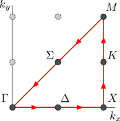
Figure 2: A plot of the symmetry points in the first Brillouin zone. The arrows show the path taken in plotting the energy spectra in Fig. 3, starting from the origin at $\Gamma=\!\left(0,0\right)$.

Using the method outlined in Section VI above, the models in Eq. 12 and Eq. 14 have been solved by exact diagonalization on 16-site lattices with periodic boundary conditions. We start by considering the vector Hamiltonian given by Eq. 12. The spectrum is shown in Fig. 3; the points in the Brillouin zone which label the axis of this figure are shown in Fig. 2. We find the spectrum to be positive semi-definite, with a doubly-degenerate zero-energy state at the $\Gamma$ point. The rest of the spectrum is well separated from the ground state by a gap that is substantial and we believe not due to finite size effects in the calculation. This claim is based on the fact that it exceeds the finite size level splitting of the spectrum by a factor of $\sim 15$. The presence of a gap is expected between the chiral spin liquid ground state and what should be a two-spinon excited state. The spinon excitations of this model will be addressed in future work.

We now discuss the two orthogonal zero-energy eigenstates. For comparison, we construct the CSL state Eq. 2 explicitly and find a two-dimensional subspace of functions with the center of mass variable being treated as an external parameter. We have computed the overlap of the Hamiltonian ground state subspace and the CSL subspace and find that they match perfectly. Therefore, the ground state of this Hamiltonian is indeed the two-fold degenerate CSL state. Additionally, we have only two zero-energy states, by which follows that the CSL state is the only ground state of the model, a statement which cannot be achieved analytically.

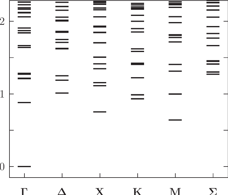
Figure 3: Low energy spectrum of the Hamiltonian Eq. 12, scaled down to order of unity. There are two $E=0$ eigenvalues at the $\Gamma$ point.

For the tensor Hamiltonian, however, we find that the zero-energy subspace is massively degenerate. It of course contains the CSL, in accord with the analytical proof, but also many additional states. While the restriction to small system sizes prevents us from studying the thermodynamic limit precisely, our numerical findings indicate that the Hamiltonian Eq. 14 does not stabilize the CSL state as the unique ground state, which thus singles out the model in Eq. 12 to be subject of further study.

VIII Conclusion

In this work we have shown a method for constructing parent Hamiltonians for the chiral spin liquid. We have computed the spectra of the Hamiltonians by use of a Kernel-sweeping method in exact diagonalization. There, for the Hamiltonian operator composed of the spherical vector component of the CSL destruction operator, we observe that the CSL states are the only ground states of the model. We conclude that this model is a promising candidate to also study the elementary excitations of the model, i.e., spinons, and many other questions in the field of two-dimensional fractionalization of quantum numbers in spin systems.

Appendix A Tensor decomposition

The operators $\omega_{j}$ introduced in Section IV may be decomposed into irreducible spherical tensors of ranks $1$ and $3$. We write these irreducible operators as $T^{q}_{m}$; $q$ and $m$ correspond to angular momentum and its $z$ component respectively. We wish to write $\omega=\sum c_{q}\,T^{q}$, where $T^{q}$ is the collection of all operators which transform as a spherical tensor of rank $q$. Here we have suppressed the site index on the operator $\omega$.

The operator in Eq. 7 that is not manifestly the component of a vector is $S_{i}^{z}\,S_{j}^{z}\,S_{k}^{z}$, which is a component of a third-rank Cartesian tensor. In order to keep the notation manageable, we start by considering the direct product of two operators $U$ and $V$ with angular momentum $j_{1}$ and $j_{2}$ respectively. An element in the direct product space of these operators may be written as

$$U^{j_{1}}_{m_{1}}\,V^{j_{2}}_{m_{2}}=\sum_{j_{12}=\left|j_{2}-j_{1}\right|}^{j_{1}+j_{2}}\,\sum_{m_{12}=-j_{12}}^{j_{12}}\,C\!\,_{j_{1}}^{m_{1}}\!\,{}_{j_{2}}^{m_{2}}\!\,{}_{j_{12}}^{m_{12}}\,T^{j_{12}}_{m_{12}}$$ (61)

in terms of irreducible spherical tensors $T_{m_{12}}^{j_{12}}$ carrying angular momentum $j_{12}$ with $z$-component $m_{12}=m_{1}+m_{2}$. Eq. 61 may be inverted to give

$$T_{m_{12}}^{j_{12}}=\sum_{m_{1}=-j_{1}}^{j_{1}}\sum_{m_{2}=-j_{2}}^{j_{2}}C\!\,_{j_{1}}^{m_{1}}\!\,{}_{j_{2}}^{m_{2}}\!\,{}_{j_{12}}^{m_{12}}\,U^{j_{1}}_{m_{1}}\,V^{j_{2}}_{m_{2}}\,.$$ (62)

Using these equations, one may construct corresponding expressions for the product of three vector operators by applying Eq. 61 twice:

$$U_{m_{1}}^{j_{1}}\,V_{m_{2}}^{j_{2}}\,W_{m_{3}}^{j_{3}} = \sum_{j_{12}=-\left|j_{1}-j_{2}\right|}^{j_{1}+j_{2}}\sum_{m_{12}=-j_{12}}^{j_{12}}C\!\,_{j_{1}}^{m_{1}}\!\,{}_{j_{2}}^{m_{2}}\!\,{}_{j_{12}}^{m_{12}}\,T_{m_{12}}^{j_{12}}\,W^{j_{3}}_{m_{3}}$$ (63)

$$= \sum_{j_{12}=-\left|j_{1}-j_{2}\right|}^{j_{1}+j_{2}}\sum_{m_{12}=-j_{12}}^{j_{12}}\,C\!\,_{j_{1}}^{m_{1}}\!\,{}_{j_{2}}^{m_{2}}\!\,{}_{j_{12}}^{m_{12}}\,\sum_{j=\left|j_{12}-j_{3}\right|}^{j_{12}+j_{3}}\sum_{m=-j}^{j}C\!\,_{j_{12}}^{m_{12}}\!\,{}_{j_{3}}^{m_{3}}\!\,{}_{j}^{m}\,T^{j\,\!\left(j_{12}\right)}_{m}\,.$$

The second superscript on the tensor $T$ in the last line distinguishes between the different tensors of the same rank that appear when combining three vector operators; since $1\otimes 1\otimes 1=3\oplus 2\oplus 2\oplus 1\oplus 1\oplus 1\oplus 0$, there are two rank-2 spherical tensors and three vector operators that can be formed. For the case of interest $m_{1}=m_{2}=m_{3}=0$ and $j_{1}=j_{2}=j_{3}=1$, the expression reduces to

$$U^{z}\,V^{z}\,W^{z}=\sum_{j_{12}=0}^{2}\sum_{j=\left|j_{12}-1\right|}^{j_{12}+1}C\!\,_{1}^{0}\!\,{}_{1}^{0}\!\,{}_{j_{12}}^{0}\,C\!\,_{j_{12}}^{0}\!\,{}_{1}^{0}\!\,{}_{j}^{0}\,T_{0}^{j\,\!\left(j_{12}\right)}=-\frac{1}{\sqrt{3}}\,T^{1\,\!\left(0\right)}_{0}-\frac{2}{\sqrt{15}}\,T^{1\,\!\left(2\right)}_{0}+\sqrt{\frac{2}{5}}\,T^{3}_{0}\,,$$ (64)

which shows that the operator contains only vector and rank-3 tensor components, but no scalar or rank-2 tensor components. Note that the second index on the rank-3 tensor has been suppressed since the construction of this object is unambiguous.

Applying Eq. 62 twice, the rank-$3$ tensor component is

$$T^{3}_{0} = \sum_{m_{12}=-2}^{2}\sum_{m_{3}=-1}^{1}C\!\,_{2}^{m_{12}}\!\,{}_{1}^{m_{3}}\!\,{}_{3}^{0}\,T^{2}_{m_{12}}\,W^{1}_{m_{3}}$$ (65)

$$= \sum_{m_{1},m_{2},m_{3}=-1}^{1}\,C\!\,_{2}^{-m_{3}}\!\,{}_{1}^{m_{3}}\!\,{}_{3}^{0}\,C\!\,_{1}^{m_{1}}\!\,{}_{1}^{m_{2}}\!\,{}_{2}^{-m_{3}}U^{1}_{m_{1}}\,V^{1}_{m_{2}}\,W^{1}_{m_{3}}$$ (66)

$$= \frac{5\,U^{z}\,V^{z}\,W^{z}-\!\left(\bm{U}\cdot\bm{V}\right)\,W^{z}-\!\left(\bm{V}\cdot\bm{W}\right)\,U^{z}-\!\left(\bm{W}\cdot\bm{U}\right)\,V^{z}}{\sqrt{10}}\,,$$ (67)

where we have used the fact that the dot product is $\mathbf{U}\cdot\mathbf{V}=\sum_{m}\!\left(-1\right)^{m}U^{1}_{m}\,V^{1}_{-m}$ in the spherical representation. A similar construction can be used to find the vector operator or, one may note from Eqs. 64 and 67 that the vector component is equivalent to

$$U^{z}\,V^{z}\,W^{z}-\sqrt{\frac{2}{5}}\,T_{0}^{3}=\frac{\!\left(\bm{U}\cdot\bm{V}\right)\,W^{z}+\!\left(\bm{V}\cdot\bm{W}\right)\,U^{z}+\!\left(\bm{W}\cdot\bm{U}\right)\,V^{z}}{5}$$ (68)

as used in writing down Eq. 11.

Construction of the remaining ($x$ and $y$) components of the vector operator in Eq. 68 is straightforward since one merely replaces $z$ with either $x$ or $y$. In order to construct the remaining six components of the rank-3 tensor operator one simply applies Eq. 62 twice without specifying $m=0$:

$$T_{m}^{3}=\sum_{m_{1},m_{2},m_{3}=-1}^{1}C\!\,_{2}^{m-m_{3}}\!\,{}_{1}^{m_{3}}\!\,{}_{3}^{m}\,C\!\,_{1}^{m_{1}}\!\,{}_{1}^{m_{2}}\!\,{}_{2}^{m-m_{3}}\,U^{1}_{m_{1}}\,V^{1}_{m_{2}}\,W^{1}_{m_{3}}\,.$$ (69)

The explicit form of these components are

$$T_{1}^{3} = -\frac{1}{2\,\sqrt{30}}\,\left[\!\left(5\,V^{z}\,W^{z}-\bm{V}\cdot\bm{W}\right)\,U^{+}+\!\left(5\,U^{z}\,W^{z}-\bm{U}\cdot\bm{W}\right)\,V^{+}+\!\left(5\,U^{z}\,V^{z}-\bm{U}\cdot\bm{V}\right)\,W^{+}\right]$$ (70)

$$T_{2}^{3} = \frac{1}{2\,\sqrt{3}}\,\left[U^{+}\,V^{+}\,W^{z}+U^{+}\,V^{z}\,W^{+}+U^{z}\,V^{+}\,W^{+}\right]$$ (71)

$$T_{3}^{3} = -\frac{1}{2\,\sqrt{2}}\,U^{+}\,V^{+}\,W^{+}\,,$$ (72)

with the remaining three components obtained from $T^{q}_{-m}=\!\left(-1\right)^{m}\,\!\left(T^{q}_{m}\right)^{\dagger}$.

Appendix B Sum Rule

The sum rule used in Section V, on which the proof that $\omega$ destroys the ground state hinges, is given by

$$\lim_{R\rightarrow\infty}\sum_{0\leq\left|z\right|<R}G\!\left(z\right)\,z^{n}\,e^{-\frac{\pi}{2}\,\left|z\right|^{2}}=0\,.$$ (73)

The sum rule has been first stated in a mathematical framework of coherent state systems by Perelomov and has later been re-derived by Laughlin perelomov71tmp156 ; laughlin89ap163 ; in this appendix, we show how to obtain the sum rule by application of Jacobi’s imaginary transformation. We first consider the related sum

$$F\!\left(c\right)=\lim_{R\rightarrow 0}\sum_{0\leq\left|z\right|<R}G\!\left(z\right)\,\exp\left[\frac{1}{2}\,c\,z-\frac{\pi}{2}\,\left|z\right|^{2}\right]\,.$$ (74)

In order to prove the sum rule in Eq. 73, we will first show that $F\!\left(c\right)=0$ for any value of the parameter $c$ and then use this to prove Eq. 73 by taking derivatives of the function $F\!\left(c\right)$.

In order to show that $F\!\left(c\right)=0$, we use the gauge function $G\!\left(z\right)$ to write Eq. 74 as two sums, one over the entire lattice and one over the points $z^{\prime}$ on the lattice for which $G\!\left(z^{\prime}\right)=-1$. As shown in Figure 2, these sites defines a sublattice with twice the original lattice spacing.

$$F\!\left(c\right)=\sum_{z}e^{\frac{1}{2}\,c\,z-\frac{\pi}{2}\,\left|z\right|^{2}}-2\,\sum_{z^{\prime}}e^{\frac{1}{2}\,c\,z^{\prime}-\frac{\pi}{2}\,\left|z^{\prime}\right|^{2}}\,.$$ (75)

Setting $z^{\prime}=2\,z$ we can write this as

$$F\!\left(c\right)=\sum_{z}e^{\frac{1}{2}\,c\,z-\frac{\pi}{2}\,\left|z\right|^{2}}-2\,\sum_{z}e^{c\,z-2\,\pi\,\left|z\right|^{2}}\,,$$ (76)

where both sums now run over the entire lattice. Writing $z=x+i\,y$ this function can be factored into four sums over the integers $x$ and $y$:

$$F\!\left(c\right) = \!\left(\sum_{x}e^{\frac{1}{2}\,\!\left(c\,x-\pi\,x^{2}\right)}\right)\,\!\left(\sum_{y}e^{\frac{1}{2}\!\left(i\,c\,y-\pi\,y^{2}\right)}\right)$$ (77)

$$-2\,\!\left(\sum_{x}e^{c\,x-2\,\pi\,x^{2}}\right)\,\!\left(\sum_{y}e^{i\,c\,y-2\,\pi\,y^{2}}\right)\,.$$

In terms of the third Jacobi theta functionAbramowitzStegun65

$$\theta_{3}\!\left(z|\tau\right)=\sum_{n=-\infty}^{\infty}e^{i\,\pi\,n^{2}\,\tau}\,e^{2\,i\,n\,z}\,,$$ (78)

this function may be recast as

$$F\!\left(c\right) = \vartheta_{3}\!\left(\left.\!-i\,\frac{c}{4}\right|\frac{i}{2}\right)\,\vartheta_{3}\!\left(\left.\!\frac{c}{4}\right|\frac{i}{2}\right)$$ (79)

$$-2\,\vartheta_{3}\!\left(\left.\!-i\,\frac{c}{2}\right|2\,i\right)\,\vartheta_{3}\!\left(\left.\!\frac{c}{2}\right|2\,i\right)\,.$$

The fact that the two terms in this expression precisely cancel is a result of Jacobi’s imaginary transformation Whittaker-58 ,

$$\theta_{3}\!\left(z|\tau\right)=\frac{1}{\sqrt{-i\,\tau}}\,e^{z^{2}/i\,\pi\,\tau}\,\vartheta_{3}\!\left(\!\left.\pm\frac{z}{\tau}\right|-\frac{1}{\tau}\right)\,,$$ (80)

and the fact that the third Jacobi theta function is even. Application of this identity to either product of theta functions in Eq. 79 shows that the two terms precisely cancel, proving that $F\!\left(c\right)=0$. This in turn proves the $n=0$ case of Eq. 73 by simply setting $c=0$. The other instances of the sum rule are obtained by noting that

$$\frac{1}{m!}\frac{d^{m}}{dc^{m}}F\!\left(c\right)=\lim_{R\rightarrow\infty}\sum_{0\leq\left|z\right|<R}G\!\left(z\right)\,z^{m}\,e^{c\,z}\,e^{-\frac{\pi}{2}\,\left|z\right|^{2}}\,.$$ (81)

Since $F\!\left(c\right)$ is $0$ for all values of $c$, setting $c=0$ in the above expression gives the desired result in Eq. 73. It should be noted that this proof can be generalized for arbitrary lattices. However, for lattice structures with non-orthogonal vectors spanning the unit cell, a decomposition into Jacobi Theta functions is not possible anymore and to follow the above line of proof one has to apply the generalized Liouville theorem for two-dimensional Riemann theta functions Mumford83 .

B.0.1 Corollary to Sum Rule

We now consider the case where we wish to evaluate a sum of the form

$$\lim_{R\rightarrow\infty}\sum_{0<\left|z\right|<R}\,\frac{1}{z}\,A\!\left(z\right)\,G\!\left(z\right)\,e^{-\frac{\pi}{2}\,\left|z\right|^{2}}$$ (82)

where $A\!\left(z\right)$ is an analytic function of $z$. Since it is analytic, we can expand the function $A\!\left(z\right)$ in a Taylor series:

$$A\!\left(z\right)=\sum_{\ell=0}^{\infty}\frac{1}{\ell!}\,\left.\frac{d^{\ell}A}{dz^{\ell}}\right|_{0}\,z^{\ell}$$ (83)

and, so long as the sum in Eq. 82 is absolutely convergent, we can interchange the order of the two infinite sums to obtain

$$\sum_{\ell}\,\frac{1}{\ell!}\,\left.\frac{d^{\ell}A}{dz^{\ell}}\right|_{0}\,\!\left(\lim_{R\rightarrow\infty}\sum_{0<\left|z\right|<R}z^{\ell-1}\,G\!\left(z\right)\,e^{-\frac{\pi}{2}\,\left|z\right|^{2}}\right)\,.$$ (84)

All terms for which $\ell>2$ immediately vanish from the interior sum due to the sum rule in Eq. 73. The term with $\ell=0$ also vanishes because in that case the summand is an odd function summed over the entire lattice. Finally the term with $\ell=1$ can be evaluated using the sum rule and is simply the negative of the value of the summand at $z=0$ (which is not included in this sum but is included in Eq. 73). Therefore, so long as $A\!\left(z\right)$ is chosen so that the sum itself is absolutely convergent,

$$\lim_{R\rightarrow\infty}\sum_{0<\left|z\right|<R}\,\frac{1}{z}\,A\!\left(z\right)\,G\!\left(z\right)\,e^{-\frac{\pi}{2}\,\left|z\right|^{2}}=\left.\frac{dA}{dz}\right|_{0}\,.$$ (85)

Appendix C The function $A\!\left(z\right)$

The ratio of wave function coefficients appearing in Eq. 33,

$$\frac{\left\langle z_{1}\cdots z_{j}+x\cdots z_{M}|\psi\right\rangle}{\left\langle z_{1}\cdots z_{j}\cdots z_{M}|\psi\right\rangle}\,,$$ (86)

can be written in terms of the Gauge function $G\!\left(x\right)$, the Gaussian $e^{-\frac{\pi}{2}\,\left|x\right|^{2}}$, and an analytic function of $x$, $A\!\left(x\right)$. To see this we note that this ratio may be written explicitly as

$$\prod_{\nu=1}^{2}\frac{\vartheta\!\left(\frac{\pi}{L}\,\left[\mathcal{Z}+x-Z_{\nu}\right]\right)}{\vartheta\!\left(\frac{\pi}{L}\,\left[\mathcal{Z}-Z_{\nu}\right]\right)}\,\prod_{i\neq j}^{M}\,\frac{\vartheta^{2}\!\left(\frac{\pi}{L}\,\left[z_{j}+x-z_{i}\right]\right)}{\vartheta^{2}\!\left(\frac{\pi}{L}\,\left[z_{j}-z_{i}\right]\right)}\,\frac{G\!\left(z_{j}+x\right)}{G\!\left(z_{j}\right)\,G\!\left(x\right)}\,\frac{e^{\frac{\pi}{2}\,\left[\,\!\left(z_{j}+x\right)^{2}-\left|z_{j}+x\right|^{2}\right]}}{e^{\frac{\pi}{2}\,\left[z_{j}^{2}-\left|z_{j}\right|^{2}\right]}\,e^{\frac{\pi}{2}\,\left[x^{2}-\left|x\right|^{2}\right]}}\,G\!\left(x\right)\,e^{\frac{\pi}{2}\,\!\left(x^{2}-\left|x\right|^{2}\right)}\,.$$ (87)

This simplifies by noting that the exponential terms obey an addition formula

$$\frac{e^{\frac{\pi}{2}\,\left[\,\!\left(z_{j}+x\right)^{2}-\left|z_{j}+x\right|^{2}\right]}}{e^{\frac{\pi}{2}\,\left[z_{j}^{2}-\left|z_{j}\right|^{2}\right]}\,e^{\frac{\pi}{2}\,\left[x^{2}-\left|x\right|^{2}\right]}}=e^{\frac{\pi}{2}\,\left[\,\!\left(x-x^{*}\right)\,z_{j}+x\,\!\left(z_{j}-z_{j}^{*}\right)\right]},$$ (88)

and the Gauge function obeys an addition formula given by

$$\frac{G\!\left(z_{j}+x\right)}{G\!\left(z_{j}\right)\,G\!\left(x\right)}=-e^{\frac{\pi}{2}\,\!\left(z_{j}^{*}\,x^{*}-z_{j}\,x\right)}\,.$$ (89)

Since the terms involving $x^{*}$ cancel on multiplying the two expressions in Eqs. 88 and 89, the ratio of coefficients is

$$\frac{\left\langle z_{1}\cdots z_{j}+x\cdots z_{M}|\psi\right\rangle}{\left\langle z_{1}\cdots z_{j}\cdots z_{M}|\psi\right\rangle}=-A\!\left(x\right)\,G\!\left(x\right)\,e^{-\frac{\pi}{2}\,\left|x\right|^{2}}\,,$$ (90)

where $A\!\left(x\right)$ is an analytic function of $x$:

$$A\!\left(x\right)=\prod_{\nu=1}^{2}\frac{\vartheta\!\left(\frac{\pi}{L}\,\left[\mathcal{Z}+x-Z_{\nu}\right]\right)}{\vartheta\!\left(\frac{\pi}{L}\,\left[\mathcal{Z}-Z_{\nu}\right]\right)}\,\prod_{i\neq j}^{M}\,\frac{\vartheta^{2}\!\left(\frac{\pi}{L}\,\left[z_{j}+x-z_{i}\right]\right)}{\vartheta^{2}\!\left(\frac{\pi}{L}\,\left[z_{j}-z_{i}\right]\right)}\,e^{\frac{\pi}{2}\,\left[x^{2}+x\,\!\left(z_{j}-z_{j}^{*}\right)\right]}\,.$$ (91)

The derivative of this function is given by

$$\frac{dA}{dx}=\left\{\sum_{\nu=1}^{2}\frac{d}{dx}\ln\vartheta\!\left(\frac{\pi}{L}\,\left[\mathcal{Z}+x-Z_{\nu}\right]\right)+2\,\sum_{i\neq j}^{M}\frac{d}{dx}\ln\vartheta\!\left(\frac{\pi}{L}\,\left[z_{j}-z_{i}+x\right]\right)+\frac{\pi}{2}\,\!\left(2\,x+z_{j}-z_{j}^{*}\right)\right\}\,A\!\left(x\right)\,.$$ (92)

Evaluating this at $x=0$ and noting that $A\!\left(0\right)=1$ from Eq. 91 gives

$$\left.\frac{dA}{dx}\right|_{0}=\sum_{\nu=1}^{2}\frac{d}{d\mathcal{Z}}\ln\vartheta\!\left(\frac{\pi}{L}\,\left[\mathcal{Z}-Z_{\nu}\right]\right)+2\,\sum_{i\neq j}^{M}\frac{d}{dz_{j}}\ln\vartheta\!\left(\frac{\pi}{L}\,\left[z_{j}-z_{i}\right]\right)+N\,\frac{\pi}{L}\,\frac{z_{j}-z_{j}^{*}}{2\,L}\,.$$ (93)

In terms of the function $W\!\left(z\right)$ introduced in Eq. 17 this may be written as

$$\left.\frac{dA}{dx}\right|_{0}=\sum_{\nu=1}^{2}\frac{\pi}{L}\,W\!\left(\frac{\pi}{L}\,\left[\mathcal{Z}-Z_{1}\right]\right)+2\,\sum_{i\neq j}^{M}\frac{\pi}{L}W\!\left(\frac{\pi}{L}\left[z_{j}-z_{i}\right]\right)\,.$$ (94)

The final expression follows from the fact that the center of mass zeroes are constrained to satisfy $\sum_{\nu}Z_{\nu}=0$ as pointed out in Section II.

References

- (1) W. P. Su, J. R. Schrieffer, and A. J. Heeger, Phys. Rev. Lett. 42, 1698 (1979).
- (2) J. M. Leinaas and J. Myrheim, Nuovo Cimento B 37, 1 (1977).
- (3) F. Wilczek, Phys. Rev. Lett. 48, 1144 (1982).
- (4) F. Wilczek, Phys. Rev. Lett. 49, 957 (1982).
- (5) R. B. Laughlin, Phys. Rev. Lett. 50, 1395 (1983).
- (6) B. I. Halperin, Phys. Rev. Lett. 52, 1583 (1984), ibid. 52, E2390 (1984).
- (7) D. Arovas, J. R. Schrieffer, and F. Wilczek, Phys. Rev. Lett. 53, 722 (1984).
- (8) F. Wilczek, Fractional statistics and anyon superconductivity (World Scientific, Singapore, 1990).
- (9) V. J. Goldman and B. Su, Science 267, 1010 (1995).
- (10) R. de Picciotto, M. Reznikov, M. Heiblum, V. Umansky, G. Bunin, and D. Mahalu, Nature 389, 162 (1997).
- (11) M. Reznikov, R. de Picciotto, T. G. Griffiths, M. Heiblum, and V. Umansky, Nature 399, 238 (1999).
- (12) F. E. Camino, W. Zhou, and V. J. Goldman, Phys. Rev. Lett. 95, 246802 (2005).
- (13) D. E. Feldman, Y. Gefen, A. Kitaev, K. T. Law, and A. Stern, Phys. Rev. B 76, 085333 (2007).
- (14) F. D. M. Haldane, Phys. Rev. Lett. 67, 937 (1991).
- (15) M. Greiter, Phys. Rev. B 79, 064409 (2009).
- (16) F. D. M. Haldane, Phys. Rev. Lett. 60, 635 (1988).
- (17) B. S. Shastry, Phys. Rev. Lett. 60, 639 (1988).
- (18) F. D. M. Haldane, Phys. Rev. Lett. 66, 1529 (1991).
- (19) F. D. M. Haldane, Z. N. C. Ha, J. C. Talstra, D. Bernard, and V. Pasquier, Phys. Rev. Lett. 69, 2021 (1992).
- (20) D. A. Tennant, T. G. Perring, R. A. Cowley, and S. E. Nagler, Phys. Rev. Lett. 70, 4003 (1993).
- (21) R. Coldea, D. A. Tennant, R. A. Cowley, D. F. McMorrow, B. Dorner, and Z. Tylczynski, Phys. Rev. Lett. 79, 151 (1997).
- (22) B. J. Kim et al., Nature Physics 2, (2006).
- (23) C. Nayak and K. Shtengel, Phys. Rev. B 64, 064422 (2001).
- (24) G. Misguich, D. Serban, and V. Pasquier, Phys. Rev. Lett. 89, 137202 (2002).
- (25) R. Moessner and S. L. Sondhi, Phys. Rev. Lett. 86, 1881 (2001).
- (26) P. W. Anderson, Science 235, 1197 (1987).
- (27) S. A. Kivelson, D. S. Rokhsar, and J. P. Sethna, Phys. Rev. B 35, 8865 (1987).
- (28) A. Y. Kitaev, Ann. Phys. 303, 2 (2002).
- (29) V. Kalmeyer and R. B. Laughlin, Phys. Rev. Lett. 59, 2095 (1987).
- (30) V. Kalmeyer and R. B. Laughlin, Phys. Rev. B 39, 11879 (1989).
- (31) X. G. Wen, Phys. Rev. B 40, 7387 (1989).
- (32) X. G. Wen, F. Wilczek, and A. Zee, Phys. Rev. B 39, 11413 (1989).
- (33) H. Yao and S. A. Kivelson, Phys. Rev. Lett. 99, 247203 (2007).
- (34) A. Kitaev, Ann. of Phys. 321, 2 (2006).
- (35) M. Greiter and R. Thomale, Phys. Rev. Lett. 102, 207203 (2009).
- (36) N. Read and E. Rezayi, Phys. Rev. B 59, 8084 (1999).
- (37) D. F. Schroeter, E. Kapit, R. Thomale, and M. Greiter, Phys. Rev. Lett. 99, 097202 (2007).
- (38) F. D. M. Haldane and E. H. Rezayi, Phys. Rev. B 31, 2529 (1985).
- (39) Handbook of Mathematical Functions, edited by M. Abramowitz and I. A. Stegun (Dover, New York, 1965).
- (40) R. B. Laughlin, Ann. Phys. 191, 163 (1989).
- (41) A. M. Perelomov, Theoret. Math. Phys. 6, 156 (1971).
- (42) E. T. Whittaker and G. N. Watson, A course of Modern Analysis (Cambridge University Press, Cambridge, 1958 (5th edition)).
- (43) D. Mumford, Tata Lectures on Theta (Birkhäuser, Basel, 1983), Vol. I and II.