Concavity of the quantum body for any given dimension

Abstract

Let us consider the set of all joint probabilities generated by local binary measurements on two separated quantum systems of a given local dimension $d$. We address the question of whether the shape of this quantum body is convex or not. We construct a point in the space of joint probabilities, which is on the convex hull of the local polytope, but still cannot be attained by measuring $d$-dimensional quantum systems, if the number of measurement settings is large enough. From this it follows that this body is not convex. We also show that for finite $d$ the quantum body with POVM allowed may contain points that can not be achieved with only projective measurements.

Quantum correlations are points in the space of correlations which are achievable in quantum phyics by performing local measurements on separate quantum systems. In contrast, classical correlations can be achieved by local strategies using shared randomness. For a given number of measurement inputs and outputs the set of classical correlations forms a convex polytope Froissart . However, we have learned from the theorem of John Bell that there exist quantum correlations that lie outside this polytope Bell . Thus the set of quantum correlations (which we refer to as the quantum body) is strictly larger than the set of classical correlations.

Let us first consider the quantum body consisting of two spacelike separated parties, each having a choice of performing two measurements with two outputs. If we keep only joint correlations in the set (excluding marginal terms), we obtain the simplest nontrivial quantum body. The boundary of this set has already been described by Tsirelson Tsirelson , notably, deriving the maximal quantum violation for the Clauser-Horne-Shimony-Holt (CHSH) inequality CHSH . Subsequent works corr22 characterized the boundary of this quantum domain in different but essentially equivalent ways. Recently, the structure of this body has been the subject of analytical study in Ref. Pit08 deriving quadratic inequalities. However, the fact that in this quantum body marginal terms are not included, the inequalities derived can give only partial information on the full probability distribution, i.e., on the shape of the whole quantum body for two parties with two inputs and two outputs.

Beyond this scenario, Navascués et al. NPA07 devised a sophisticated method based on a hierarchy of semidefinite relaxations. This is completely general, in that it can be applied to any number of parties, performing measurements with any number of inputs and outputs. However, the method in its present form works efficiently for the case when no constraints are imposed on the dimension of the system. In absence of such a powerful program, the shape of the quantum body for a fixed dimension is not well understood. It is not even known whether it is convex or concave. Without the restriction for the dimensionality of the quantum systems the quantum body is proven to be convex Pit89 ; WW . It is also known, that the size of the quantum body may grow with $d$ for two parties dimwitness ; VP09 ; higherdim and for three parties as well Perez .

In the present paper we wish to further advance the study on the shape of the quantum body corresponding to a fixed Hilbert space dimension $d$ of bipartite systems. We address the problem recently raised by Navascués et al. NPA08 : Is the shape of the quantum body convex for a restricted dimension $d$? Our main result shows that even by four two-outcome measurement settings per party the corresponding quantum body for a pair of two-dimensional quantum systems (qubits) is concave. This result holds for the most general POVM measurements and for projective measurements as well and can be generalized beyond qubits to any dimension $d$.

Preliminaries. Let Alice and Bob have two components of a compound physical system. Let Alice and Bob choose one of a set of $m_{A}$ and $m_{B}$ two-outcome measurements, respectively, and let them perform the measurement chosen on their respective subsystems. Let us denote the outcome of Alice’s measurement $i$ and Bob’s measurement $j$ by $A_{i}=\pm 1$ ($i=1,\dots,m_{A}$) and $B_{j}=\pm 1$ ($j=1,\dots,m_{B}$), respectively. Let us denote the vector having components $\langle A_{i}\rangle$, $\langle B_{j}\rangle$ and $\langle A_{i}B_{j}\rangle$ for all $i$ and $j$ by $\bf x\in\mathbb{R}^{m_{A}+m_{B}+m_{A}m_{B}}$, where $\langle\cdot\rangle$ denotes the expected value. Vector $\bf x$ may be measured by repeating the procedure above on many copies of the system, making sure that each pair of measurements $(i,j)$ is chosen to be performed a sufficient number of times to get a satisfactory statistics. The actual vector one gets will depend on the physical system and on the measurement settings the parties are allowed to choose from. We note that $\langle A_{i}\rangle$ and $\langle B_{j}\rangle$ is only defined sensibly if the probability of getting a measurement outcome by one party does not depend on which measurement the other party has chosen. This is the requirement of no-signaling, which is true in both classical and quantum physics, and believed to be true in Nature.

As we have mentioned above, the set of vectors one may get when making measurements on systems obeying classical physics, or any locally realistic model, is a polytope Froissart ; Pit89 . The vertices of the polytope correspond to the deterministic situations, when each $A_{i}$ and $B_{j}$ has a definite value every time it is measured, and the polytope itself is the convex hull of these points. A Bell inequality of the form $\bf M\cdot\bf x\leq K$ define an $(m_{A}+m_{B}+m_{A}m_{B}-1)$-dimensional hyperplane touching the polytope, such that the polytope is on that side of the hyperplane, which satisfies the inequality. Tight Bell inequalities are the ones that define the hyperplanes of the facets of the polytope. While all vectors $\bf x$ allowed classically may be reproduced by measurements on quantum systems, the opposite is not true. In quantum mechanics Bell inequalities may be violated, therefore the set of the vectors $\bf x$ allowed is larger. It is not a polytope, but it is still a convex set Pit89 ; WW .

In quantum mechanics the components of $\bf x$ may be calculated as $\langle A_{i}\rangle={\rm tr}(\rho\hat{A}_{i}\otimes\hat{I}_{B})$, $\langle B_{j}\rangle={\rm tr}(\rho\hat{I}_{A}\otimes\hat{B}_{j})$, and $\langle A_{i}B_{j}\rangle={\rm tr}(\rho\hat{A}_{i}\otimes\hat{B}_{j})$. Here $\hat{A}_{i}\in{\cal H}_{A}$ ($\hat{B}_{j}\in{\cal H}_{B}$) is the observable corresponding to Alice’s (Bob’s) measurement $i$ ($j$), ${\cal H}_{A}$ (${\cal H}_{B}$) is the Hilbert space associated to the subsystem of Alice (Bob), $\hat{I}_{A}\in{\cal H}_{A}$ and $\hat{I}_{B}\in{\cal H}_{B}$ are the unity operators of the respective Hilbert spaces, and $\rho\in{\cal H}_{A}\otimes{\cal H}_{B}$ is the density operator of the physical system. Operators $\hat{A}_{i}=\hat{I}_{A}-2\hat{P}^{A}_{i}$ and $\hat{B}_{j}=\hat{I}_{B}-2\hat{P}^{B}_{j}$ have eigenvalues $\pm 1$, while $\hat{P}^{A}_{i}\in{\cal H}_{A}$ and $\hat{P}^{B}_{j}\in{\cal H}_{B}$ are projection operators, whose expected values give the probability of getting outcome $-1$ for the corresponding measurements. If we do not confine ourselves to projective measurements, but we allow the more general POVM measurements, then $\hat{P}^{A}_{i}$ ($\hat{P}^{B}_{j}$) will be the POVM element associated to outcome $-1$ of the Alice’s (Bob’s) measurement $i$ ($j$), which is not necessarily a projector, but any positive operator with eigenvalues between $0$ and $1$. The relation with $\hat{A}_{i}$ ($\hat{B}_{j}$) remains the same as above.

Method. Let us arrange $X_{00}\equiv 1$, and the components of $\bf x$ into a matrix of $m_{A}+1$ rows and $m_{B}+1$ columns as $X_{i0}=\langle A_{i}\rangle$, $X_{0j}=\langle B_{j}\rangle$ and $X_{ij}=\langle A_{i}B_{j}\rangle$. The quantum mechanical expression for these matrix elements is $X_{ij}={\rm tr}(\rho\hat{A}_{i}\otimes\hat{B}_{j})$, with the definitions $\hat{A}_{0}\equiv\hat{I}_{A}$ and $\hat{B}_{0}\equiv\hat{I}_{B}$, here we allowed indices $i$ and $j$ to take value $0$. Let us restrict the dimensionality of the component Hilbert spaces ${\cal H}_{A}$ and ${\cal H}_{B}$ to two. In two dimensions all Hermitian operators can be written as a real linear combination of the three Pauli operators and the unity operator, therefore if $m_{A}>3$, there must exist an $\hat{A}_{i}$ operator which can be written as a linear combination of the other $\hat{A}_{k}$ operators and the unity operator with real coefficients. Then the row of the $X_{ij}$ matrix depending on that operator can also be written as the linear combination of the rows depending on the other $\hat{A}_{k}$ operators and the zeroth row, with the same coefficients. We can conclude that correlations described by $X_{ij}$ having more than four linearly independent rows can not be reproduced with measurements taken on a pair of qubits. We may repeat the argument for the columns, too. When we go beyond qubits, but still restrict ourselves to finite dimensional Hilbert spaces, we can draw a similar conclusion: $X_{ij}$ having more than $d^{2}$ linearly independent rows or columns can not be reproduced by measurements performed on systems with no more than $d$-dimensional component Hilbert spaces. This is because any $d$-dimensional Hermitian matrix can be characterized by $d$ real (diagonal elements) and $d(d-1)/2$ complex (nondiagonal elements) numbers, altogether $d^{2}$ real numbers, therefore, no more than $d^{2}$ of them may be linearly independent with real coefficients. The conclusion holds for both projective and POVM measurements, as only the hermiticity of the operators has been used in the argument. The inclusion of POVM is important, because as we will show, if the dimensionality of the quantum system is restricted, the quantum body can be larger if we allow POVM.

Main result. Now let us consider the set of $\bf x$ vectors achievable with measurements on quantum systems of at most $d$-dimensional component Hilbert spaces. The set is not convex, if there exist points in the vector space that belong to the set, but some point on the convex hull of these points does not. The latter can be proven by showing that the matrix $X_{ij}$ corresponding to that point has more than $d^{2}$ linearly independent columns or rows. We will prove below that if $m_{A}=m_{B}=m\geq d^{2}$ and even, the set will not even contain some vector on the convex hull of points corresponding to deterministic cases, that is an element of the local polytope. The deterministic cases can obviously be reproduced with any physical systems by using degenerate measurements, measurements with definite outcomes independent of the physical system.

We note that to express the classical or quantum limits on results of correlation experiments very often not the vectors $\bf x$, but the vectors $\bf p$ are used, whose components are $p_{A_{i}}$, $p_{B_{j}}$ and $p_{A_{i}B_{j}}$, which are the probabilities of getting outcome $-1$ for Alice’s $i$th, for Bob’s $j$th, and for both experiments, respectively. The two approaches are equivalent AII .

Let $m_{A}=m_{B}=m$ be even, and let us take all $m!/(m/2)!^{2}$ deterministic cases with the $A_{i}$ being +1 the same number of times as it is -1, and $B_{i}=-A_{i}$. Let us call the corresponding vectors and matrix elements ${\bf x}^{(\sigma)}$ and $X_{ij}^{(\sigma)}$ ($\sigma=1,\dots,m!/(m/2)!^{2}$), respectively. Let ${\bf x}^{(+)}$ and ${\bf x}^{(-)}$ be defined by $A_{i}^{(+)}=B_{i}^{(+)}=+1$ and $A_{i}^{(-)}=B_{i}^{(-)}=-1$, respectively. Let us take the following point on the convex hull of these vectors:

$${\bf x}^{o}=\frac{m-1}{m}\frac{(m/2)!^{2}}{m!}\sum_{\sigma}{\bf x}^{(\sigma)}+\frac{1}{2m}\left({\bf x}^{(+)}+{\bf x}^{(-)}\right).$$ (1)

For each deterministic strategy considered in the sum above, there is another one with the same weight with all measurement outcomes having the opposite sign, therefore $X^{o}_{i0}=X^{o}_{0j}=0$ ($i,j=1,\dots,m$). As $X_{ii}^{(\sigma)}=A_{i}^{(\sigma)}B_{i}^{(\sigma)}=-1$, and $X_{ii}^{(+)}=X_{ii}^{(-)}=+1$, it follows that $X_{ii}^{o}=(2/m)-1$. It is easy to see, that if $i\neq j$, the value of $X_{ij}^{(\sigma)}=A_{i}^{(\sigma)}B_{j}^{(\sigma)}=-A_{i}^{(\sigma)}A_{j}^{(\sigma)}$ is $+1$ for $2[(m-2)!]/(m/2-1)!^{2}$ cases, and $-1$ for the rest of them, and it is obvious that $X_{ij}^{(+)}=X_{ij}^{(-)}=+1$. From these and from Eq. (1) it follows that the nondiagonal matrix elements with indices larger than zero are $X_{ij}^{o}=2/m$. The matrix has a nonzero determinant, all $m+1$ rows and columns are linearly independent, therefore, if $d^{2}\leq m$, ${\bf x}^{o}$ can not be reproduced by measurements performed on quantum systems with $d$-dimensional component Hilbert spaces.

Explicit Bell polynomial. Now we will show that all vectors ${\bf x}^{o}$, ${\bf x}^{(\sigma)}$, ${\bf x}^{(+)}$ and ${\bf x}^{(-)}$ considered above belong to a set that maximizes a Bell inequality, which can not be violated in quantum mechanics, so they are on the surface of both the classical polytope and the quantum set. As the quantum set has a multidimensional intersection with the polytope, it follows that its surface can not be round everywhere. This fact has been also reported recently in the work of Linden et al. Linden in the context of distributed computing. The intersection has a lower dimensionality than a facet, so the Bell inequality is not a tight one. It is a correlation type inequality, that is the factors multiplying $\langle A_{i}\rangle$ and $\langle B_{j}\rangle$ are zero. The Bell polynomial is

$${\cal B}=\sum_{i=1}^{m}\sum_{j=1}^{m}M_{ij}\langle A_{i}B_{j}\rangle\equiv\sum_{i=1}^{m}\sum_{j=1}^{m}\left(1-\frac{m}{2}\delta_{ij}\right)\langle A_{i}B_{j}\rangle,$$ (2)

where $\delta_{ij}$ is the Kronecker delta. To get the maximum value of this expression it is enough to consider pure states and projective measurements. It is proven in AGT06 that for any observables $\hat{A}$ and $\hat{B}$ in Alice’s and Bob’s component spaces, respectively, and state $\psi$ there exist Euclidean vector $\vec{a}$ independent of $\hat{B}$ and vector $\vec{b}$ independent of $\hat{A}$ such that $\langle AB\rangle=\langle\psi|\hat{A}\otimes\hat{B}|\psi\rangle=\vec{a}\cdot\vec{b}$. Therefore, we may replace $\langle A_{i}B_{j}\rangle$ with $\vec{a}_{i}\cdot\vec{b}_{j}$ in Eq. (2), and maximize that expression. The vectors $\vec{a}_{i}$ have to be chosen such that they are parallel with the vectors they are multiplied with. Then we get:

$$\vec{a}_{i} ={\frac{1}{l_{i}}}\left(\sum_{j=1}^{m}\vec{b}_{j}-\frac{m}{2}\vec{b}_{i}\right),$$ (3)

$${\cal B} =\sum_{i=1}^{m}l_{i}=\sum_{i=1}^{m}\left|\sum_{j=1}^{m}\vec{b}_{j}-\frac{m}{2}\vec{b}_{i}\right|=$$ (4)

$$=\sum_{i=1}^{m}\sqrt{\frac{m^{4}}{4}+\sum_{j=1}^{m}\vec{b}_{j}\cdot\sum_{k=1}^{m}\vec{b}_{k}-m\vec{b}_{i}\cdot\sum_{k=1}^{m}\vec{b}_{k}}.$$ (5)

We will show that we get the maximum value for $\cal B$ if

$$(\vec{b}_{i}-\vec{b}_{j})\cdot\sum_{k=1}^{m}\vec{b}_{k}=0$$ (6)

is true for any $i$ and $j$. Then one can see from Eqs. (4,5) that $l_{i}=m/2$, and ${\cal B}=m^{2}/2$. This agrees with the upper limit this Bell expression may take with quantum measurements, as it can be shown analytically making use of semidefinite programming technique. The actual proof, following Wehner’s work Wehner is deferred to Appendix .1.

From Ref. VP09 it follows, that if $m_{A}=m_{B}$, and the maximum value of the Bell expression can be achieved with all $\vec{b}_{j}$ are linearly independent, than this solution can not be unique. The present case is an example for this situation. Equation (6) has an infinite number of solutions, with $\vec{b}_{j}$ spanning spaces of any dimensionality up to $m$. An obvious one-dimensional solution is when all $\vec{b}_{j}$ are chosen to be the same unit vector $\vec{b}$. Then from Eq. (3) and $l_{i}=m/2$ it follows that $\vec{a}_{i}=\vec{b}$. This arrangement corresponds to the classical deterministic strategies of having all measurement outcomes either $+1$ or $-1$ every time (correlation vectors ${\bf x}^{(+)}$ and ${\bf x}^{(-)}$). If $m$ is even, there are further one dimensional solutions, with half the $\vec{b}_{j}$ pointing to one direction and the other half pointing to the opposite direction. Such a solution corresponds to a deterministic strategy in which Bob has as many measurements with a definite outcome of $+1$ as ones with an outcome of $-1$, and Alice gets the outcome $A_{i}=-B_{i}$ for each $i$ (correlation vectors ${\bf x}^{(\sigma)}$). From the existence of classical deterministic strategies giving the quantum limit for the Bell expression it follows that the Bell inequality can not be violated.

There is an infinite number of solutions of Eq. (6) with $\vec{b}_{j}$ spanning the maximum of $m$ dimensions. An arrangement with all $\vec{b}_{j}$ are orthogonal to each other is one of them. Then $\vec{a}_{i}$ are also orthogonal to each other, and $\langle A_{i}B_{j}\rangle=\vec{a}_{i}\cdot\vec{b}_{j}=(2/m)-\delta_{ij}$, (see Eq. (3)). According to Tsirelson’s construction these values can be realized as quantum expectation values of $\pm 1$ valued observables with a maximally entangled state of a system of $2^{m/2}$ dimensional component Hilbert spaces Tsirelson . With this state the expectation values $\langle A_{i}\rangle=0$ and $\langle B_{j}\rangle=0$. By choosing the unit vectors corresponding to the unity operators in the component Hilbert spaces orthogonal to the space spanned by $\vec{b}_{j}$, we can get all components of the correlation vector as dot products. This correlation vector is nothing else than ${\bf x}^{o}$, which we have chosen to construct on the convex hull of the set of classical deterministic cases ${\bf x}^{(\sigma)}$, ${\bf x}^{(+)}$ and ${\bf x}^{(-)}$ according to Eq. (1) as an example that can not be achieved with quantum systems of component spaces of $d\leq\sqrt{m}$ dimensions. Clearly, we could have chosen an infinite number of other vectors with the required property.

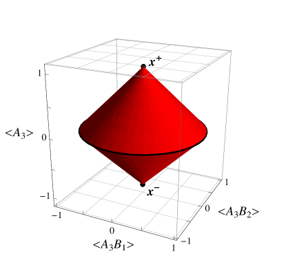
Figure 1: (Color online) Quantum region in the three-dimensional section spanned by the expectation values $\langle A_{3}B_{1}\rangle$, $\langle A_{3}B_{2}\rangle$ and $\langle A_{3}\rangle$ as described in the text. The two antipodal apices of the cones, corresponding to ${\bf x^{+}}$ and ${\bf x^{-}}$, and the equator (in black color) can be attained by projective measurements performed on qubits. Whereas, any other point on the surface of the cone (represented by red color) can be achieved by applying POVM measurements.

POVM versus projective measurements. Now we will show that the quantum body with POVM allowed may contain points that can not be achieved with only projective measurements. Let us consider the quantum body with $m_{A}=3$ and $m_{B}=2$, restricting ourselves to quantum systems of two dimensional component Hilbert spaces. Let $\hat{A}_{1}$, $\hat{A}_{2}$, $\hat{B}_{1}$ and $\hat{B}_{2}$ be the operators, and $|\psi\rangle$ be the pure maximally entangled state giving the maximum violation of the CHSH inequality. Let the components $\langle A_{i}\rangle$, $\langle B_{j}\rangle$ and $\langle A_{i}B_{j}\rangle$ ($i,j=1,2$) of $\bf x$ be derived as the expectation values of the operators above. Let the components $\langle A_{3}\rangle$, $\langle A_{3}B_{1}\rangle$ and $\langle A_{3}B_{2}\rangle$ be the expectation values with $\hat{A}_{3}$ corresponding to a projective measurement, that is an observable with eigenvalues $\pm 1$. Then it can be shown that the region allowed for these three components are the two antipodal apices of the cones ${\bf x}^{+}$ and ${\bf x}^{-}$ (when $\hat{A}_{3}=\hat{I}_{A}$ and $\hat{A}_{3}=-\hat{I}_{A}$, respectively) and the equator of unit radius (when $\hat{A}_{3}$ has both eigenvalues $+1$ and $-1$), shown in Fig. 1. To see this, one has to to use the facts that to get the other, fixed components of the vector the state must be maximally entangled and the relationship between $\hat{B}_{1}$ and $\hat{B}_{2}$ is also well defined. For example, ${\bf x}^{\lambda}=\lambda{\bf x}^{+}+(1-\lambda){\bf x}^{-}$ ($0<\lambda<1$), a point between the antipodes, can not be achieved, as the expectation value of $\hat{A}_{3}$ calculated with a maximally entangled state can only be $\pm 1$ or $0$, and when it is $0$, $\langle A_{3}B_{1}\rangle$ and $\langle A_{3}B_{2}\rangle$ can not be $0$ at the same time. However, we do achieve the point required with the choice of $\hat{A}_{3}^{\lambda}=(2\lambda-1)\hat{I}_{A}$. This operator corresponds to a POVM with POVM elements $\lambda\hat{I}_{A}$ and $(1-\lambda)\hat{I}_{A}$ associated with the +1 and -1 outcome of the measurement, respectively. Similarly, it is easy to prove that all other points within the red region shown in Fig. 1 can be attained with POVM.

Conclusion. We proved that the full set of quantum probabilities in the bipartite scenario generated either by two-outcome projective or by two-outcome POVM measurements for any given dimension $d$ is concave. However, one may further ask, whether this fact also holds true for more parties and for more than two outcomes. We also proved that the set generated by projective measurements may be smaller than the one corresponding to the more general POVM measurements. In case of two-outcome measurements the maximum violation of a Bell inequality with fixed dimensional systems can still be achieved with projective measurements CHTW04 ; LD . It remains an open question if this is true in cases of more than two outcomes Gisin07 .

A further question raised by Brunner et al. BGS is that what happens, if we restrict ourselves to measurements on a given quantum state and look for the set of quantum probabilities generated this way. When we limit the dimensionality of the Hilbert space, we have shown here that the quantum set is concave, by showing that a point on the convex hull of points corresponding to deterministic strategies does not belong to the set if the number of measurement settings is large enough. By restricting ourselves to a particular state, the set can only get smaller, while it will still contain the points of deterministic strategies.

Finally, it would also be interesting to find out the minimum number of settings which generates a quantum body with a concave shape for a fixed dimension. In particular, would it be possible in the bipartite case to go below four two-outcome measurement settings per party by local dimension two in order to prove concavity of the corresponding quantum body?

.1 Appendix: Quantum maximum via SDP

We follow the SDP method put forward by Wehner Wehner recently, in order to prove analytically quantum bounds for the correlation type Bell inequalities of Eq. (2). Let us consider the $m\times m$ matrix $M$ with real coefficients

$$M_{ij}=1-\frac{m}{2}\delta_{ij},$$ (7)

introduced in Eq. (2). As stated in the main text, the expectation values in the polynomial Eq. (2) can be replaced by dot product of unit vectors,

$$\max{\sum_{i,j=1}^{m}{M_{ij}\vec{a}_{i}\cdot\vec{b}_{j}}},$$ (8)

where maximization is taken over all unit vectors $\{\vec{a}_{1},\ldots,\vec{a}_{m},\vec{b}_{1},\ldots,\vec{b}_{m}\}\in R^{2m}$. As shown by Tsirelson, the maximum obtained in this way corresponds to the maximum quantum value as well Tsirelson .

However, the above problem can be formulated as the following SDP optimization Wehner :

maximize $$\quad\frac{1}{2}\mathsf{Tr}{(\Gamma W)}$$ (9)

subject to $$\quad\Gamma\succeq 0,\quad\forall i\,\Gamma_{ii}=1\,.$$

Here the matrix $W$ is built up as

$$W=\left(\begin{array}[]{cc}0&M\\ M&0\end{array}\right),$$ (12)

and $\Gamma=(\Gamma_{ij})$ is the Gram matrix of the unit vectors $\{\vec{a}_{1},\ldots,\vec{a}_{m},\vec{b}_{1},\ldots,\vec{b}_{m}\}\in R^{2m}$. Denoting the columns of the above vectors by $V$, we can write $\Gamma=V^{t}V$ if and only if $\Gamma$ is positive semidefinite. The constraint $\Gamma_{ii}=1$, on the other hand, owes to the unit length of vectors $\vec{a}_{i}$ and $\vec{b}_{j}$. Note, that the primal problem defined by (9) is the first step of the hierarchy of semidefinite programs given by Navascués et al. NPA07 ; NPA08 .

However, one can also define a dual formulation of the SDP problem (for an exhaustive review see VB04 ):

maximize $$\quad\mathsf{Tr}{(\mathop{\mathrm{diag}}(\lambda))}$$ (13)

subject to $$\quad-\frac{1}{2}W+\mathop{\mathrm{diag}}(\lambda)\succeq 0,$$

where $\lambda$ is a $2m$-dimensional vector with real entries and we note that this dual problem is just the first step of the hierarchy introduced by Doherty et al. DLTW .

Let us denote by $p^{*}$ and $d^{*}$ the optimal values for the primal and the dual problems, respectively. However, according to weak duality, $d^{*}\geq p^{*}$ VB04 . Thus, in order to prove optimality of the quantum bound one suffices to exhibit a feasible solution both for the primal (9) and for the dual (13) problem and then show that they are in fact equal to each other. For this sake let us guess the primal optimum by setting $\vec{a}_{i},\vec{b}_{j}=(1,0,\ldots,0)$ in (8) with a Bell matrix defined by (7). These vectors correspond to a classical deterministic strategy and this solution yields $p^{*}=\sum_{i,j}^{m}{M_{i,j}}=m^{2}/2$.

Similarly, we guess the solution $\lambda^{*}=(m/4)(1,\ldots,1)$ for the dual problem, for which the dual value is $d^{*}=\mathsf{Tr}{(\mathop{\mathrm{diag}}(\lambda^{*}))}=m^{2}/2$. In order to get a feasible solution, it remains to check according to (13) whether $R=-(1/2)W+\mathop{\mathrm{diag}}(\lambda^{*})\succeq 0$ is satisfied. This amounts to prove $\gamma_{min}[R]\geq 0$, where we use the notation $\gamma_{min}[R]$ ($\gamma_{max}[R]$) for the smallest (largest) eigenvalue of a matrix $R$. However, due to Weyl’s theorem HJ85 , for two Hermitian matrices $P$ and $Q$, it holds $\gamma_{min}[P+Q]\geq\gamma_{min}[P]+\gamma_{min}[Q]$. For our particular case,

$$\gamma_{min}[R] \geq\gamma_{min}[-\frac{1}{2}W]+\gamma_{min}[\mathop{\mathrm{diag}}(\lambda^{*})]$$

$$=-\frac{1}{2}\gamma_{max}[W]+\frac{m}{4}.$$ (14)

The eigenvalues of matrix $W$ in the form (12) are given by the singular values $\sigma_{s}=\sqrt{\gamma_{s}\gamma_{s}^{*}}$ of matrix $M$ of (7) and their negatives. The eigenvalues of $M$ on the other hand are the roots of the characteristic polynomial $\mathrm{det}(M-\gamma_{s}\leavevmode\hbox{\small 1\normalsize\kern-3.30002pt1})$, where 11 is the $m\times m$ unit matrix. In VP09 we found that the determinant of an $m\times m$ matrix with diagonal elements $p$ and non-diagonal elements $q$ is $[p+(m-1)q](p-q)^{m-1}$. By inserting $p=1-m/2-\gamma_{s}$ and $q=1$ into the determinant above, we obtain the roots $\gamma_{s}=\pm m/2$. This result implies $\gamma_{max}[W]=\frac{m}{2}$. By substituting this value into (14) we get $\gamma_{min}[R]\geq 0$. This implies that this solution for $d^{*}$ is feasible, and recalling the guessed solution $p^{*}$, we have $d^{*}=p^{*}$. Thus the maximum quantum value of the Bell polynomial $M$ defined by Eq. (2) is equal to $m^{2}/2$, which can be achieved by classical means as well.