Accuracy of Quasicontinuum Approximations
Near Instabilities

Abstract.

The formation and motion of lattice defects such as cracks, dislocations, or grain boundaries, occurs when the lattice configuration loses stability, that is, when an eigenvalue of the Hessian of the lattice energy functional becomes negative. When the atomistic energy is approximated by a hybrid energy that couples atomistic and continuum models, the accuracy of the approximation can only be guaranteed near deformations where both the atomistic energy as well as the hybrid energy are stable. We propose, therefore, that it is essential for the evaluation of the predictive capability of atomistic-to-continuum coupling methods near instabilities that a theoretical analysis be performed, at least for some representative model problems, that determines whether the hybrid energies remain stable up to the onset of instability of the atomistic energy.

We formulate a one-dimensional model problem with nearest and next-nearest neighbor interactions and use rigorous analysis, asymptotic methods, and numerical experiments to obtain such sharp stability estimates for the basic conservative quasicontinuum (QC) approximations. Our results show that the consistent quasi-nonlocal QC approximation correctly reproduces the stability of the atomistic system, whereas the inconsistent energy-based QC approximation incorrectly predicts instability at a significantly reduced applied load that we describe by an analytic criterion in terms of the derivatives of the atomistic potential.

1. Introduction

An important application of atomistic-to-continuum coupling methods is the study of the quasistatic deformation of a crystal in order to model instabilities such as dislocation formation during nanoindentation, crack growth, or the deformation of grain boundaries [18]. In each of these applications, the quasistatic evolution provides an accurate approximation of the crystal deformation until the evolution approaches an unstable configuration. This occurs, for example, when a dislocation forms or moves or when a crack tip advances. The crystal will then typically undergo a dynamic process until it reaches a new stable configuration. In order to guarantee an accurate approximation of the entire quasistatic crystal deformation, up to the formation of an instability, it is crucial that the equilibrium in the atomistic/continuum hybrid method is stable whenever the corresponding atomistic equilibrium is. The purpose of this work is to investigate whether the quasicontinuum (QC) method has this property. In technical terms, this requires sharp estimates on the stability constant in the QC approximation.

The QC method is an atomistic-to-continuum coupling method that models the continuum region by using an energy density that exactly reproduces the lattice-based energy density at uniform strain (the Cauchy-Born rule) [18, 21, 25]. Several variants of the QC approximation have been proposed that differ in how the atomistic and continuum regions are coupled [3, 8, 18, 26]. In this paper, we present sharp stability analyses for the main examples of conservative QC approximations as a means to evaluate their relative predictive properties for defect formation and motion. Our sharp stability analyses compare the loads for which the atomistic energy is stable, that is, those loads where the Hessian of the atomistic energy is positive-definite, with the loads for which the QC energies are stable. It has previously been suggested and then observed in computational experiments that inconsistency at the atomistic-to-continuum interface can reduce the accuracy for computing a critical applied load [25, 18, 19, 8]. In this paper, we give an analytical method to estimate the error in the critical applied load by deriving stability criteria in terms of the derivatives of the atomistic potential.

Although we present our techniques in a precise mathematical format, we believe that these techniques can be utilized in a more informal way by computational scientists to quantitatively evaluate the predictive capability of other atomistic-to-continuum or multiphysics models as they arise. For example, our quantitative approach has the potential to estimate the reduced critical applied load in QC approximations such as the quasi-nonlocal QC approximation (QNL), that are consistent for next-nearest interactions but not for longer range interactions. Since the longer range interactions are generally weak, such an estimate may give an analytical basis to judging that the reduced critical applied load for QNL with finite range interactions is within an acceptable error tolerance.

The accuracy of various QC approximations and other atomistic-to-continuum coupling methods is currently being investigated by both computational experiments and numerical analysis  [1, 2, 4, 5, 7, 9, 11, 12, 14, 15, 16, 20, 23, 24]. The main issue that has been studied to date in the mathematical analyses is the rate of convergence with respect to the smoothness of the continuum solution (however, see [2, 7, 23] for analyses of the error of the QC solutions with respect to the atomistic solution, possibly containing defects). Some error estimates have been obtained that give theoretical justification for the accuracy of a QC approximation for all loads up to the critical atomistic load where the atomistic model loses stability [5, 23], but other error estimates that have been presented do not hold near the atomistic limit loads. It is important to understand whether the break-down of these error estimates is an artifact of the analysis, or whether the particular QC approximation actually does incorrectly predict an instability before the applied load has reached the correct limit load of the atomistic model.

Two key ingredients in any approximation error analysis are the consistency and stability of the approximation scheme. For energy minimization problems, consistency means that the truncation error for the equilibrium equations is small in a suitably chosen norm, and stability is usually understood as the positivity of the Hessian of the functional. For the highly non-convex problems we consider here, stability must necessarily be a local property: The configuration space can be divided into stable and unstable regions, and the question we ask is whether the stability regions of different QC approximations approximate the stability region of the full atomistic model in a way that can be controlled in the setup of the method (for example, by a judicious choice of the atomistic region).

In this work, we initiate such a systematic study of the stability of QC approximations. In the present paper, we investigate conservative QC approximations, that is, QC approximations which are formulated in terms of the minimization of an energy functional. In a companion paper [6], we study the stability of a force-based approach to atomistic-to-continuum coupling that is nonconservative.

In computational experiments, one often studies the evolution of a system under incremental loading. There, the critical load at which the system “jumps” from one energy well to another is often the goal of the computation. Thus, we will also study the effect of the “stability error” on the error in the critical load.

We will formulate a simple model problem, a one dimensional periodic atomistic chain with pairwise next-nearest neighbour interactions of Lennard-Jones type, for which we can analyze the issues layed out in the previous paragraphs. It is well known that the uniform configuration is stable only up to a critical value of the tensile strain (fracture). We use analytic, asymptotic, and numerical approaches to obtain sharp results for the stability of different QC approximations when applied to this simple model.

In Section 2, we describe the model and the various QC approximations that we will analyze. In Section 4, we study the stability of the atomistic model as well as two consistent QC approximations: the local QC approximation (QCL) and the quasi-nonlocal QC approximation (QNL). We prove that the critical applied strains for both of these approximations are equal to the critical applied strain for the atomistic model, up to second-order in the atomistic spacing.

A similar analysis for the inconsistent QCE approximation is more difficult because the uniform configuration is not an equilibrium. Thus, in Section 5, we construct a first-order correction of the uniform configuration to approximate an equilibrium configuration, and we study the positive-definiteness of the Hessian for the linearization about this configuration. We explicitly construct a test function with strain concentrated in the atomistic-continuum interface that is unstable for applied strains bounded well away from the atomistic critical applied strain.

In Section 6, we analyze the accuracy in predicting the critical strain for onset of instability. For the QCL and QNL approximations, this involves comparing the effect of the difference between their modified stability criteria and that of the atomistic model. For QCE, since the solution to the nonlinear equilibrium equations are non-trivial, we provide computational results in addition to an analysis of the critical QCE strain predicted by the approximations derived in Section 5.

2. The atomistic and quasicontinuum models

2.1. The atomistic model problem

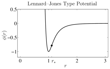
Figure 1. Lennard-Jones type interaction potential. The bond length $r_{*}$ is the turning point between the convex and concave regions of $\phi$.

Suppose that the infinite lattice $\varepsilon\mathbb{Z}$ is deformed uniformly into the lattice $y_{F}:=F\varepsilon\mathbb{Z},$ where $F>0$ is the macroscopic deformation gradient and where $\varepsilon>0$ scales the reference atomic spacing, that is,

$$(y_{F})_{\ell}:=F\ell\varepsilon\quad\text{for }-\infty<\ell<\infty.$$

We admit $2N$-periodic perturbations $u=(u_{\ell})_{\ell\in\mathbb{Z}}$ from the uniformly deformed lattice $y_{F}.$ More precisely, for fixed $N\in\mathbb{N}$, we admit deformations $y$ from the space

$$\mathcal{Y}_{F}:=\big{\{}y\in\mathbb{R}^{\mathbb{Z}}:y=y_{F}+u,\,u\in\mathcal{U}\big{\}},$$

where $\mathcal{U}$ is the space of $2N$-periodic displacements with zero mean,

$$\mathcal{U}:=\big{\{}u\in\mathbb{R}^{\mathbb{Z}}:u_{\ell+2N}=u_{\ell}\text{ for }\ell\in\mathbb{Z},\text{ and }{\textstyle\sum_{\ell=-N+1}^{N}}u_{\ell}=0\big{\}}.$$

We set $\varepsilon=1/N$ throughout so that the reference length of the periodic domain is fixed. Even though the energies and forces we will introduce are well-defined for all $2N$-periodic displacements, we require that they have zero mean in order to obtain locally unique solutions to the equilibrium equations. These zero mean constraints are an artifact of our periodic boundary conditions and are similarly used in the analysis of continuum problems with periodic boundary conditions.

We assume that the stored energy per period of a deformation $y\in\mathcal{Y}_{F}$ is given by a next-nearest neighbour pair interaction model,

$$\mathcal{E}_{\rm a}(y):=\varepsilon\sum_{\ell=-N+1}^{N}\big{(}\phi(y_{\ell}^{\prime})+\phi(y_{\ell}^{\prime}+y_{\ell+1}^{\prime})\big{)},$$ (1)

where $v_{\ell}^{\prime}$ is the backward difference

$$v_{\ell}^{\prime}:=\varepsilon^{-1}(v_{\ell}-v_{\ell-1})\qquad\text{for }v\in\mathbb{R}^{\mathbb{Z}},\ \ell\in\mathbb{Z},$$

and where $\phi$ is a Lennard-Jones type interaction potential satisfying (see also Figure 1)

1. $\phi\in{\rm C}^{4}((0,+\infty);\mathbb{R})$,

2. there exists $r_{*}>0$ such that $\phi$ is convex in $(0,r_{*})$ and concave in $(r_{*},+\infty)$, and

3. $\phi^{(k)}(r)\rightarrow 0$ rapidly as $r\nearrow\infty$, for $k=0,\dots,4$.

We have used the scaled interaction potential, $\varepsilon\phi(r/\varepsilon),$ in the definition of the stored energy, $\mathcal{E}_{\rm a}(y),$ to obtain a continuum limit as $\varepsilon\to 0.$ Assumptions (i) and (ii) are used throughout our analysis, while assumption (iii) serves primarily to motivate that next-nearest neighbour interaction terms are typically dominated by nearest-neighbour terms. Note, however, that even with assumption (iii), the relative size of next-nearest and nearest neighbour interactions is comparable when strains approach $r_{*}$.

We denote the first variation of the energy functional, $\mathcal{E}_{\rm a}^{\prime}(y)[u],$ at a deformation $y\in\mathcal{Y}_{F}$ by

$$\mathcal{E}_{\rm a}^{\prime}(y)[u]:=\sum_{\ell=-N+1}^{N}\frac{\partial\mathcal{E}_{\rm a}(y)}{\partial y_{\ell}}u_{\ell}=\varepsilon\sum_{\ell=-N+1}^{N}\Big{\{}\phi^{\prime}(y_{\ell}^{\prime})u_{\ell}^{\prime}+\phi^{\prime}(y_{\ell}^{\prime}+y_{\ell+1}^{\prime})(u_{\ell}^{\prime}+u_{\ell+1}^{\prime})\Big{\}},$$

for $u\in\mathcal{U}$. In the absence of external forces, the uniformly deformed lattice $y=y_{F}$ is an equilibrium of the atomistic energy under perturbations from $\mathcal{U}$, that is,

$$\mathcal{E}_{\rm a}^{\prime}(y_{F})[u]=0\qquad\text{ for all }u\in\mathcal{U}.$$ (2)

We identify the stability of $y_{F}$ with linear stability under perturbations from the space $\mathcal{U}$. To make this precise, we denote the second variation of the energy functional, $\mathcal{E}_{\rm a}^{\prime\prime}(y)[u,v],$ evaluated at a deformation $y\in\mathcal{Y}_{F}$, by

$$\begin{split}\mathcal{E}_{\rm a}^{\prime\prime}(y)[u,v]&:=\sum_{\ell,\,m=-N+1}^{N}\frac{\partial^{2}\mathcal{E}_{\rm a}(y)}{\partial y_{\ell}\partial y_{m}}u_{\ell}v_{m}\\ &=\varepsilon\sum_{\ell=-N+1}^{N}\Big{\{}\phi^{\prime\prime}(y_{\ell}^{\prime})u_{\ell}^{\prime}v_{\ell}^{\prime}+\phi^{\prime\prime}(y_{\ell}^{\prime}+y_{\ell+1}^{\prime})[u_{\ell}^{\prime}+u_{\ell+1}^{\prime}][v_{\ell}^{\prime}+v_{\ell+1}^{\prime}]\Big{\}},\end{split}$$ (3)

for all $u,v\in\mathcal{U}$. The matrix $\Big{(}\frac{\partial^{2}\mathcal{E}_{\rm a}(y)}{\partial y_{\ell}\partial y_{m}}\Big{)}_{\ell,m=-N+1}^{N}$ is the Hessian for the energy functional. We say that the equilibrium $y_{F}$ is stable for the atomistic model if this Hessian, evaluated at $y=y_{F}$, is positive definite on the subspace $\mathcal{U}$ of zero mean displacements, or equivalently, if

$$\mathcal{E}_{\rm a}^{\prime\prime}(y_{F})[u,u]>0\qquad\text{ for all }u\in\mathcal{U}\setminus\{0\}.$$ (4)

In Section 3, Definition 3, we extend this definition of stability to the various QC approximation and their equilibria.

Note that if $y=y_{F}$, then $y_{\ell}^{\prime}=F$ and $y_{\ell}^{\prime}+y_{\ell+1}^{\prime}=2F$ for all $\ell$. Therefore, upon defining the quantities

$$\phi_{F}^{\prime\prime}:=\phi^{\prime\prime}(F),\quad\phi_{2F}^{\prime\prime}:=\phi^{\prime\prime}(2F),\quad\text{and}\quad A_{F}=\phi_{F}^{\prime\prime}+4\phi_{2F}^{\prime\prime},$$

we can rewrite (3) as follows

$$\mathcal{E}_{\rm a}^{\prime\prime}(y_{F})[u,u]=\varepsilon\sum_{\ell=-N+1}^{N}\big{\{}\phi_{F}^{\prime\prime}|u_{\ell}^{\prime}|^{2}+\phi_{2F}^{\prime\prime}|u_{\ell}^{\prime}+u_{\ell+1}^{\prime}|^{2}\big{\}}\quad\text{for }u\in\mathcal{U}.$$ (5)

(We will use $A_{F}$ later.) The quantities $\phi_{F}^{\prime\prime}$ and $\phi_{2F}^{\prime\prime}$ will play a prominent role in the analysis of the stability of the atomistic model and its QC approximations and describe the strength of the nearest neighbor and next-nearest neighbor interactions, respectively. We similarly define the quantities $\phi^{(k)}_{G}$ for all $k\in\mathbb{N}$ and for all $G>0$. For most realistic interaction potentials the second-nearest neighbour coefficient is non-positive, $\phi_{2F}^{\prime\prime}\leq 0,$ except in the case of extreme compression (see Figure 1). Therefore, in order to avoid having to distinguish several cases, we will assume throughout our analysis that $F\geq r_{*}/2$. In this case, property (ii) of the interaction potential shows that $\phi_{2F}^{\prime\prime}\leq 0$.

We also note that, for $u\in\mathcal{U}$, both $u^{\prime}$ and $u^{\prime\prime}$ are understood as $2N$-periodic chains, that is, $u^{\prime},u^{\prime\prime}\in\mathcal{U},$ where the centered second difference $u^{\prime\prime}\in\mathcal{U}$ is defined by

$$u_{\ell}^{\prime\prime}:=\varepsilon^{-2}(u_{\ell+1}-2u_{\ell}+u_{\ell-1})\qquad\text{for }u\in\mathbb{R}^{\mathbb{Z}},\ \ell\in\mathbb{Z}.$$

For $u,v\in\mathcal{U}$, we also define the weighted $\ell^{p}$-norms

$$\|v\|_{\ell^{p}_{\varepsilon}}:=\left\{\begin{array}[]{rl}\displaystyle\Bigg{(}\sum_{\ell=-N+1}^{N}\varepsilon|v_{\ell}|^{p}\Bigg{)}^{1/p},&1\leq p<\infty,\\[10.0pt] \displaystyle\max_{\ell=-N+1,\dots,N}|v_{\ell}|,&p=\infty,\end{array}\right.$$

as well as the weighted $\ell^{2}$-inner product

$$\langle u,v\rangle=\varepsilon\sum_{\ell=-N+1}^{N}u_{\ell}v_{\ell}.$$

2.2. The local QC approximation (QCL)

Before we introduce different flavors of QC approximations, we note that we can rewrite the atomistic energy as a sum over the contributions from each atom,

$$\mathcal{E}_{\rm a}(y)=~{} \varepsilon\sum_{\ell=-N+1}^{N}E^{a}_{\ell}(y)\qquad\text{where}$$

$$E^{a}_{\ell}(y):=~{} {\textstyle\frac{1}{2}}\big{[}\phi(y_{\ell}^{\prime})+\phi(y_{\ell+1}^{\prime})+\phi(y_{\ell-1}^{\prime}+y_{\ell}^{\prime})+\phi(y_{\ell+1}^{\prime}+y_{\ell+2}^{\prime})\big{]}.$$

If $y$ is “smooth,” i.e., $y_{\ell}^{\prime}$ varies slowly, then $E^{a}_{\ell}(y)\approx E^{c}_{\ell}(y)$ where

$$E^{c}_{\ell}(y):={\textstyle\frac{1}{2}}\big{[}\phi(y_{\ell}^{\prime})+\phi(y_{\ell+1}^{\prime})+\phi(2y_{\ell}^{\prime})+\phi(2y_{\ell+1}^{\prime})\big{]}={\textstyle\frac{1}{2}}\big{[}\phi_{cb}(y_{\ell}^{\prime})+\phi_{cb}(y_{\ell+1}^{\prime})\big{]},$$

and where $\phi_{cb}(r):=\phi(r)+\phi(2r)$ is the so-called Cauchy-Born stored energy density. In this case, we may expect that the atomistic model is accurately represented by the local QC (or continuum) model

$$\mathcal{E}_{\rm qcl}(y):=\varepsilon\sum_{\ell=-N+1}^{N}E^{c}_{\ell}(y)=\varepsilon\sum_{\ell=-N+1}^{N}\phi_{cb}(y_{\ell}^{\prime}).$$ (6)

The main feature of this continuum model is that the next-nearest neighbour interactions have been replaced by nearest neighbour interactions, thus yielding a model with more locality. Such a model can subsequently be coarse-grained (i.e., degrees of freedom are removed) which yields efficient numerical methods.

2.3. The energy-based QC approximation (QCE)

If $y_{\ell}^{\prime}$ is “smooth” in the majority of the computational domain, but not in a small neighbourhood, say, $\{-K,\dots,K\}$, where $K>1$, then we can obtain sufficient accuracy and efficiency by coupling the atomistic model to the local QC model by simply choosing energy contributions $E^{a}_{\ell}$ in the atomistic region $\mathcal{A}=\{-K,\dots,K\}$ and $E^{c}_{\ell}$ in the continuum region $\mathcal{C}=\{-N+1,\dots,N\}\setminus\mathcal{A}$. This approximation of the atomistic energy is often called the energy based QC approximation [21] and yields the energy functional

$$\mathcal{E}_{\rm qce}(y):= \varepsilon\sum_{\ell\in\mathcal{C}}E^{c}_{\ell}(y)+\varepsilon\sum_{\ell\in\mathcal{A}}E^{a}_{\ell}(y).$$

It is now well-understood [3, 4, 5, 8, 25] that the QCE approximation exhibits an inconsistency (“ghost force”) near the interface, which is displayed in the fact that $\mathcal{E}_{\rm qce}^{\prime}(y_{F})\neq 0.$ The first remedy of this lack of consistency was the ghost force correction scheme [25] which eventually led to the derivation of the force-based QC approximation [3] and which we analyze in [6] and [7].

2.4. Quasi-nonlocal coupling (QNL)

An alternative approach was suggested in [26], which requires a modification of the energy at the interface. This idea is best understood in terms of interactions rather than energy contributions of individual atoms (see also [8] where this has been extended to longer range interactions). The nearest neighbour interactions are left unchanged. A next-nearest neighbour interaction $\phi(\varepsilon^{-1}(y_{\ell+1}-y_{\ell-1}))$ is left unchanged if at least one of the atoms $\ell+1,\ell-1$ belong to the atomistic region and is replaced by a Cauchy–Born approximation,

$$\phi(\varepsilon^{-1}(y_{\ell+1}-y_{\ell-1}))\approx{\textstyle\frac{1}{2}}\big{[}\phi(2y_{\ell}^{\prime})+\phi(2y_{\ell+1}^{\prime})]$$

if both atoms belong to the continuum region. This idea leads to the energy functional

$$\begin{split}\mathcal{E}_{\rm qnl}(y):=\varepsilon\sum_{\ell=-N+1}^{N}\phi(y_{\ell}^{\prime})+\varepsilon\sum_{\ell\in\mathcal{A}_{\rm qnl}}\phi(y_{\ell}^{\prime}+y_{\ell+1}^{\prime})+\varepsilon\sum_{\ell\in\mathcal{C}_{\rm qnl}}{\textstyle\frac{1}{2}}\big{[}\phi(2y_{\ell}^{\prime})+\phi(2y_{\ell+1}^{\prime})\big{]}\end{split}$$

where $\mathcal{A}_{\rm qnl}=\{-K-1,\dots,K+1\}$ and $\mathcal{C}_{\rm qnl}=\{-N+1,\dots,N\}\setminus\mathcal{A}_{\rm qnl}$ are modified atomistic and continuum regions. The QNL approximation is consistent, that is, $y=y_{F}$ is an equilibrium of the QNL energy functional. The label QNL comes from the original intuition of considering interfacial atoms as quasi-nonlocal, i.e., they interact by different rules with atoms in the atomistic and continuum regions.

3. Stability of Quasicontinuum Approximations: Summary

In this section, we briefly summarize the our main results.

We begin by giving a careful definition of a notion of stability. Our condition is slightly stronger than local minimality, which is the natural concept of stability in statics. However, an analysis of local minimality alone is usually not tractable. Moreover, for the deformations that we consider, our definition is in fact sufficiently general.

Definition 1 (Stable Equilibrium). Let $\mathcal{E}:\mathcal{Y}_{F}\to\mathbb{R}\cup\{+\infty\}$. We say that $y\in\mathcal{Y}_{F}$ is a stable equilibrium of $\mathcal{E}$ if $\mathcal{E}$ is twice differentiable at $y$ and the following conditions hold:

• $\mathcal{E}^{\prime}(y)[u]=0$ for all $u\in\mathcal{U}$,

• $\mathcal{E}^{\prime\prime}(y)[u,u]>0$ for all $u\in\mathcal{U}\setminus\{0\}$.

If only (i) holds, then we call $y$ a critical point of $\mathcal{E}$.

We focus on the deformation $y_{F}=(F\ell\varepsilon)_{\ell\in\mathbb{Z}}$ and ask for which macroscopic strains $F$ this deformation is a stable equilibrium. We know from (2) that $y_{F}$ is a critical point of the atomistic energy $\mathcal{E}_{\rm a}$, and it is easy to see that $y_{F}$ is also a critical point of the QCL energy $\mathcal{E}_{\rm qcl}$ and of the QNL energy $\mathcal{E}_{\rm qnl}$. Our analysis in Section 4 gives the following conditions under which $y_{F}$ is stable:

1. $y_{F}$ is a stable equilibrium of $\mathcal{E}_{\rm a}$ if and only if $A_{F}-\varepsilon^{2}\pi^{2}\phi_{2F}^{\prime\prime}+O(\varepsilon^{4})>0$;

2. $y_{F}$ is a stable equilibrium of $\mathcal{E}_{\rm qcl}$ if and only if $A_{F}>0$;

3. $y_{F}$ is a stable equilibrium of $\mathcal{E}_{\rm qnl}$ if and only if $A_{F}>0$

where we recall that $A_{F}=\phi_{F}^{\prime\prime}+4\phi_{2F}^{\prime\prime}$ is the continuum elastic modulus for the Cauchy–Born stored energy function $\phi_{cb}(r)=\phi(r)+\phi(2r)$. Points 1., 2., and 3. are established, respectively, in Propositions 4.1, 4.2, and 4.3.

If we envision a quasistatic process in which $F$ is slowly increased, then we may wish to find the critical strain $F^{*}$ at which $y_{F}$ is no longer a stable equilibrium (fracture instability). If we denote the critical strains in the atomistic, QCL, and QNL models, respectively, by $F_{\rm a}^{*}$, $F_{\rm qcl}^{*}$ and $F_{\rm qnl}^{*}$, then 1.–3. imply that (cf. Section 6)

$$|F_{\rm a}^{*}-F_{\rm qcl}^{*}|=O(\varepsilon^{2})\quad\text{and}\quad|F_{\rm a}^{*}-F_{\rm qnl}^{*}|=O(\varepsilon^{2}).$$

For the QCE approximation defined in Section 2.3, the situation is more complicated. The occurrence of a “ghost force” in the QCE model implies that $y_{F}$ is not a critical point of $\mathcal{E}_{\rm qce}$, and consequently, we will need to analyze the stability of the second variation $\mathcal{E}_{\rm qce}^{\prime\prime}(y_{{\rm qce},F})$ where $y_{{\rm qce},F}\neq y_{F}$ is an appropriately chosen equilibrium of $\mathcal{E}_{\rm qce}$. Since $y_{{\rm qce},F}$ solves a nonlinear equation, we will replace it by an approximate equilibrium in our analysis in Section 5 where we obtain the following (simplified) result:

1. For $y_{{\rm qce},F}$ to be a stable equilibrium of $\mathcal{E}_{\rm qce}$ it is necessary that

   $$1+\frac{3\phi_{2F}^{\prime\prime}}{2\phi_{F}^{\prime\prime}}+\frac{\phi_{F}^{\prime\prime\prime}\phi_{2F}^{\prime}}{2|\phi_{F}^{\prime\prime}|^{2}}+O(\delta^{2})>0,$$

   where $\delta=\max\{|\phi^{(j)}(2F)/\phi^{\prime\prime}(F)|:j=1,2,3\}$ is assumed to be small.

We remark that 4. gives only a necessary but not a sufficient condition for stability of the QCE equilibrium $y_{{\rm qce},F}$, which, moreover, depend on assumptions on the parameter $\delta$. We refer to Remark 5 for a careful discussion of the role of $\delta$.

If we let $\tilde{F}_{\rm qce}^{*}$ denote the critical strain at which 4. fails (ignoring the $O(\delta^{2})$ term), then we obtain

$$|F_{\rm a}^{*}-\tilde{F}_{\rm qce}^{*}|=O(1),$$

which suggests that the QCE method is unable to predict the onset of fracture instability accurately. In Section 6, we confirm this asymptotic prediction with numerical experiments.

We have shown in [17] that the stability properties of the ghost force correction scheme (GFC) can be understood for uniaxial tensile loading by considering the stability of the QC energy

$$\mathcal{E}_{{\rm gfc},\,y_{F}}(y):=\mathcal{E}_{\rm qce}(y)-\mathcal{E}_{\rm qce}^{\prime}(y_{F})(y-y_{F})\quad\text{for all }y\in\mathcal{Y}_{F}.$$ (7)

We note that $\mathcal{E}_{{\rm gfc},\,y_{F}}^{\prime}(y_{F})=0,$ so $y_{F}$ is an equilibrium of the $\mathcal{E}_{{\rm gfc},\,y_{F}}$ energy under perturbations from $\mathcal{U}.$ We can therefore analyze the stability of $\mathcal{E}_{{\rm gfc},\,y_{F}}(y)$ at $y_{F}$ by studying the Hessian $\mathcal{E}_{\rm qce}^{\prime\prime}(y_{F})=\mathcal{E}_{{\rm gfc},\,y_{F}}^{\prime\prime}(y_{F}).$ We show in Remark 5 in Section 2.3 that

1. $y_{F}$ is a stable equilibrium of $\mathcal{E}_{{\rm gfc},\,y_{F}}$ if and only if $A_{F}+\lambda_{K}\phi_{2F}^{\prime\prime}>0$ where ${\textstyle\frac{1}{2}}\leq\lambda_{K}\leq 1.$

We give analytic and computation results in Sections 5 and 6 showing that the ghost force correction scheme can be expected to improve the accuracy of the computation of the critical strain by the QCE method, that is,

$$\tilde{F}_{\rm qce}^{*}<F_{\rm qce}^{y_{F}}<F_{\rm a}^{*},$$

where $F_{\rm qce}^{y_{F}}$ is the critical strain at which $\mathcal{E}_{\rm qce}^{\prime\prime}(y_{F})=\mathcal{E}_{{\rm gfc},\,y_{F}}^{\prime\prime}(y_{F})$ is no longer positive definite, but the error in computing the critical strain by the GFC scheme is still

$$|F_{\rm a}^{*}-F_{\rm qce}^{y_{F}}|=O(1).$$

4. Sharp Stability Analysis of Consistent QC Approximations

In this section, we analyze the stability of the atomistic model and two consistent QC approximations: the local QC approximation and the quasi-nonlocal QC approximation. In each case, we will give precise conditions on $F$ under which $y_{F}$ is stable in the respective approximation. The inconsistent energy-based QC approximation (QCE) is analyzed in Section 5. The corresponding result for QCE is less exact than for QCL and QNL, but shows that there is a much more significant loss of stability.

4.1. Atomistic model

Recalling the representation of $\mathcal{E}_{a}^{\prime\prime}(y_{F})$ from (5) and noting that

$$|u_{\ell}^{\prime}+u_{\ell+1}^{\prime}|^{2}=2|u_{\ell}^{\prime}|^{2}+2|u_{\ell+1}^{\prime}|^{2}-|u_{\ell+1}^{\prime}-u_{\ell}^{\prime}|^{2},$$ (8)

we obtain

$$\mathcal{E}_{a}^{\prime\prime}(y_{F})[u,u]=~{} \varepsilon\sum_{\ell=-N+1}^{N}\phi_{F}^{\prime\prime}|u_{\ell}^{\prime}|^{2}+\varepsilon\sum_{\ell=-N+1}^{N}\phi_{2F}^{\prime\prime}\big{(}2|u_{\ell}^{\prime}|^{2}+2|u_{\ell+1}^{\prime}|^{2}-|u_{\ell+1}^{\prime}-u_{\ell}^{\prime}|^{2}\big{)}$$

$$=~{} \varepsilon\sum_{\ell=-N+1}^{N}(\phi_{F}^{\prime\prime}+4\phi_{2F}^{\prime\prime})|u_{\ell}^{\prime}|^{2}+\varepsilon\sum_{\ell=-N+1}^{N}(-\varepsilon^{2}\phi_{2F}^{\prime\prime})|u_{\ell}^{\prime\prime}|^{2}$$

$$=~{} A_{F}\|u^{\prime}\|_{\ell^{2}_{\varepsilon}}^{2}+(-\varepsilon^{2}\phi_{2F}^{\prime\prime})\|u^{\prime\prime}\|_{\ell^{2}_{\varepsilon}}^{2}.$$ (9)

To quantify the influence of the strain gradient term, we define

$$\mu_{\varepsilon}:=\inf_{\psi\in\mathcal{U}\setminus\{0\}}\frac{\|\psi^{\prime\prime}\|_{2}}{\|\psi^{\prime}\|_{2}}.$$

Since $u$ is periodic, it follows that $u^{\prime}$ has zero mean. In this case, the eigenvalue $\mu_{\varepsilon}$ is known to be attained by the eigenfunction $\psi^{\prime}_{\ell}=\sin(\varepsilon\ell\pi)$ and is given by [27, Exercise 13.9]

$$\mu_{\varepsilon}=\frac{2\sin(\pi\varepsilon/2)}{\varepsilon}.$$ (10)

Since $\sin(t)=t+O(t^{3})$ as $t\searrow 0$, it follows that $\mu_{\varepsilon}=\pi+O(\varepsilon^{2})$ as $\varepsilon\searrow 0$. Thus, we obtain the following stability result for the atomistic model.

Proposition 2. Suppose $\phi_{2F}^{\prime\prime}\leq 0$. Then $y_{F}$ is stable in the atomistic model if and only if $A_{F}-\varepsilon^{2}\mu_{\varepsilon}^{2}\phi_{2F}^{\prime\prime}>0$, where $\mu_{\varepsilon}$ is the eigenvalue defined in (10).

Proof.

By the definition of $\mu_{\varepsilon}$, and using (9), we have

$$\inf_{\begin{subarray}{c}u\in\mathcal{U}\\ \|u^{\prime}\|_{\ell^{2}_{\varepsilon}}=1\end{subarray}}\mathcal{E}_{\rm a}^{\prime\prime}(y_{F})[u,u]=A_{F}-\varepsilon^{2}\phi_{2F}^{\prime\prime}\inf_{\begin{subarray}{c}u\in\mathcal{U}\\ \|u^{\prime}\|_{\ell^{2}_{\varepsilon}}=1\end{subarray}}\|u^{\prime\prime}\|_{\ell^{2}_{\varepsilon}}^{2}=A_{F}-\varepsilon^{2}\mu_{\varepsilon}^{2}\phi_{2F}^{\prime\prime}.\qed$$

4.2. The Local QC approximation

The equilibrium system, in variational form, for the QCL approximation is

$$\mathcal{E}_{\rm qcl}^{\prime}(y)[u]=\varepsilon\sum_{\ell=-N+1}^{N}\big{(}\phi^{\prime}(y_{\ell}^{\prime})+2\phi^{\prime}(2y_{\ell}^{\prime})\big{)}u_{\ell}^{\prime}=0\qquad\text{ for all }u\in\mathcal{U}.$$

Since $u^{\prime}$ has zero mean, it follows that $y=y_{F}$ is a critical point of $\mathcal{E}_{\rm qcl}$ for all $F$. The second variation of the local QC energy, evaluated at $y=y_{F}$, is given by

$$\mathcal{E}_{\rm qcl}^{\prime\prime}(y_{F})[u,u]=~{} \varepsilon\sum_{\ell=-N+1}^{N}A_{F}|u_{\ell}^{\prime}|^{2}\qquad\text{ for }u\in\mathcal{U}.$$

Thus, recalling our definition of stability from Section 2.1, we obtain the following result.

Proposition 3. The deformation $y_{F}$ is a stable equilibrium of the local QC approximation if and only if $A_{F}>0$.

Comparing Proposition 4.2 with Proposition 4.1 we see a first discrepancy, albeit small, between the stability of the full atomistic model and the local QC approximation (or the Cauchy–Born approximation). In Section 6 we will show that this leads to a negligible error in the computed critical load.

4.3. Quasi-nonlocal coupling

By the construction of the QNL coupling rule at the interface, the deformation $y=y_{F}$ is an equilibrium of $\mathcal{E}_{\rm qnl}$ [26]. The second variation of $\mathcal{E}_{\rm qnl}$ evaluated at $y=y_{F}$ is given by

$$\begin{split}\mathcal{E}_{\rm qnl}^{\prime\prime}(y_{F})[u,u]=\varepsilon\sum_{\ell=-N+1}^{N}\phi_{F}^{\prime\prime}|u_{\ell}^{\prime}|^{2}+~{}&\varepsilon\sum_{\ell\in\mathcal{A}_{\rm qnl}}\phi_{2F}^{\prime\prime}|u_{\ell}^{\prime}+u_{\ell+1}^{\prime}|^{2}\\ +~{}&\varepsilon\sum_{\ell\in\mathcal{C}_{\rm qnl}}4\phi_{2F}^{\prime\prime}({\textstyle\frac{1}{2}}|u_{\ell}^{\prime}|^{2}+{\textstyle\frac{1}{2}}|u_{\ell+1}^{\prime}|^{2}).\end{split}$$

We use (8) to rewrite the second group on the right-hand side (the nonlocal interactions) in the form

$$\varepsilon\sum_{\ell=-K-1}^{K+1}\phi_{2F}^{\prime\prime}|u_{\ell}^{\prime}+u_{\ell+1}^{\prime}|^{2}=\varepsilon\sum_{\ell=-K-1}^{K+1}\big{(}2\phi_{2F}^{\prime\prime}(|u_{\ell}^{\prime}|^{2}+|u_{\ell+1}^{\prime}|^{2})-\varepsilon^{2}\phi_{2F}^{\prime\prime}|u_{\ell}^{\prime\prime}|^{2}\big{)},$$

to obtain

$$\mathcal{E}_{\rm qnl}^{\prime\prime}(y_{F})[u,u]=\varepsilon\sum_{\ell=-N+1}^{N}A_{F}|u_{\ell}^{\prime}|^{2}+\varepsilon\sum_{\ell=-K-1}^{K+1}(-\varepsilon^{2}\phi_{2F}^{\prime\prime})|u_{\ell}^{\prime\prime}|^{2}.$$

Except in the case $K\in\{N-1,N\}$, it now follows immediately that $y_{F}$ is stable in the QNL approximation if and only if $A_{F}>0$.

Proposition 4. Suppose that $K<N-1$ and that $\phi_{2F}^{\prime\prime}\leq 0$, then $y_{F}$ is stable in the QNL approximation if and only if $A_{F}>0$.

5. Stability Analysis of the Energy-based QC approximation

We will explain in Remark 5 that there exists ${\textstyle\frac{1}{2}}\leq\lambda_{K}\leq 1$ such that

$$\mathcal{E}_{\rm qce}^{\prime\prime}(y_{F})\quad\text{is positive definite if and only if}\quad A_{F}+\lambda_{K}\phi_{2F}^{\prime\prime}>0.$$

However, $y_{F}$ is not a critical point of $\mathcal{E}_{\rm qce},$ so we must be careful in extending the previous definition of stability to the QCE approximation. We cannot simply consider the positive-definiteness of $\mathcal{E}_{\rm qce}^{\prime\prime}(y_{F}).$ Instead, we analyze the second variation $\mathcal{E}_{\rm qce}^{\prime\prime}(y_{{\rm qce},F})$ where $y_{{\rm qce},F}\in\mathcal{Y}_{F}$ solves the QCE equilibrium equations

$$\frac{\partial\mathcal{E}_{\rm qce}}{\partial y_{\ell}}(y_{{\rm qce},F})=0\quad\text{for }\ell=-N+1,\dots,N,$$

or equivalently

$$\mathcal{E}_{\rm qce}^{\prime}(y_{{\rm qce},F})[u]=0\qquad\text{ for all }u\in\mathcal{U}.$$ (11)

We will see that, when the second-neighbour interactions are small compared with the first neighbour interactions (which we make precise in Lemma 5), there is a locally unique solution $y_{{\rm qce},F}$ of the equilibrium equations, which is the correct QCE counterpart of $y_{F}$. We will then derive a stability criterion for the equilibrium deformation $y_{{\rm qce},F}.$

In Proposition 5 below, we derive an upper bound for the coercivity of $\mathcal{E}_{\rm qce}^{\prime\prime}(y_{{\rm qce},F})[u,\,u]$ with respect to the norm $\|u^{\prime}\|_{\ell^{2}_{\varepsilon}}.$ Even though the derivation of this upper bound is only rigorous for strains bounded away from the atomistic critical strain, it clearly identifies a source of instability that cannot be found by analyzing, for example, $\mathcal{E}_{\rm qce}^{\prime\prime}(y_{F})$. Moreover, we will present numerical experiments in Section 6 showing that the critical strain predicted in our following analysis gives a remarkably accurate approximation to actual QCE critical strain.

In Section 6, we consider the critical strain for each approximation, namely the point at which the appropriate equilibrium deformation (either $y_{F}$ or $y_{{\rm qce},F}$) becomes unstable. We will see later in this section, as well as in Section 6 that predicting the loss of stability for the QCE approximation using $y_{F}$ greatly underestimates the error in approximating the atomistic critical strain by the QCE critical strain.

Due to the nonlinearity and nonlocality of the interaction law, we cannot compute $y_{{\rm qce},F}$ explicitly. Instead, we will construct an approximation $\hat{y}_{{\rm qce},F}$ which is accurate whenever second-neighbour terms are dominated by first-neighbour terms. In the following paragraphs, we first present a semi-heuristic construction, motivated by the analysis in [4], and then a rigorous approximation result, the proof of which is given in Appendix B.

In (26) in the appendix, we provide an explicit representation of $\mathcal{E}_{\rm qce}^{\prime}$. Inserting $y=y_{F}$, we obtain a variational representation of the atomistic-to-continuum interfacial truncation error terms that are often dubbed “ghost forces,”

$$\begin{split}\mathcal{E}_{\rm qce}^{\prime}(y_{F})[u]&~{}=\varepsilon{\textstyle\frac{1}{2}}\phi_{2F}^{\prime}\big{\{}u_{-K-1}^{\prime}-u_{-K+1}^{\prime}-u_{K}^{\prime}+u_{K+2}^{\prime}\big{\}}\\ &~{}:=-\phi_{2F}^{\prime}\langle\hat{g}^{\prime},u^{\prime}\rangle\qquad\text{ for }u\in\mathcal{U},\end{split}$$ (12)

where

$$\hat{g}_{\ell}^{\prime}=\left\{\begin{array}[]{rl}-{\textstyle\frac{1}{2}},&\ell=-K-1,K+2,\\ {\textstyle\frac{1}{2}},&\ell=-K+1,K,\\ 0,&\text{otherwise}.\end{array}\right.$$ (13)

We note that (12) makes our claim precise that $y_{F}$ is not a critical point of $\mathcal{E}_{\rm qce}$.

Motivated by property (iii) of the interaction potential $\phi$, we will assume that the parameters

$$\delta_{1}:=\frac{\phi^{\prime}(2F)}{\phi^{\prime\prime}(F)}\quad\text{and}\quad\delta_{2}:=\frac{-\phi^{\prime\prime}(2F)}{\phi^{\prime\prime}(F)}$$

are small, and construct an approximation for $y_{{\rm qce},F}$ which is asymptotically of second order as $\delta_{1},\delta_{2}\to 0$. Although such an approximation will not be valid near the critical strain for the QCE approximation, it will give us a rough impression how the inconsistency affects the stability of the system. We note that $\delta_{1}$ is scale invariant since we used a scaled interaction potential, $\varepsilon\phi(r/\varepsilon),$ in our definition of the stored energy (1).

A non-dimensionalization of (12) shows that $y_{{\rm qce},F}=y_{F}+O(\delta_{1})$. If $\delta_{1}$ is small, then we can linearize (11) about $y_{F}$ and find the first-order correction $y_{\rm lin}\in\mathcal{Y}_{F}$, which is given by

$$\mathcal{E}_{\rm qce}^{\prime\prime}(y_{F})[y_{\rm lin}-y_{F},u]=-\mathcal{E}_{\rm qce}^{\prime}(y_{F})[u]=\phi_{2F}^{\prime}\langle\hat{g}^{\prime},u^{\prime}\rangle\qquad\text{ for all }u\in\mathcal{U}.$$ (14)

We note that this linear system is precisely the one analyzed in detail in [4]. However, instead of using the implicit representation of $y_{\rm lin}-y_{F}$ obtained there, we use the assumption that $\delta_{2}$ is small to simplify (14) further and obtain a more explicit approximation.

Writing out the bilinear form $\mathcal{E}_{\rm qce}^{\prime\prime}(y_{F})[u,u]$ explicitly (using (28) as a starting point) gives

$$\begin{split}\mathcal{E}_{\rm qce}^{\prime\prime}(y_{F})[u,u]=~{}&\dots+\varepsilon\sum_{\ell=0}^{N}\phi_{F}^{\prime\prime}|u_{\ell}^{\prime}|^{2}+\varepsilon\sum_{\ell=0}^{K-1}\phi_{2F}^{\prime\prime}|u_{\ell}^{\prime}+u_{\ell+1}^{\prime}|^{2}+\varepsilon\sum_{\ell=K+2}^{N}4\phi_{2F}^{\prime\prime}|u_{\ell}^{\prime}|^{2}\\ &+{\textstyle\frac{\varepsilon}{2}}\phi_{2F}^{\prime\prime}|u_{K}^{\prime}+u_{K+1}^{\prime}|^{2}+{\textstyle\frac{\varepsilon}{2}}\phi_{2F}^{\prime\prime}|u_{K+1}^{\prime}+u_{K+2}^{\prime}|^{2}+{\textstyle\frac{\varepsilon}{2}}4\phi_{2F}^{\prime\prime}|u_{K+1}^{\prime}|^{2},\end{split}$$ (15)

where we have only displayed the terms in the right half of the domain and indicated the terms in the left half by dots. Ignoring all terms involving $\phi_{2F}^{\prime\prime}$, which are of order $\delta_{2}$ relative to the remaining terms, we arrive at the following approximation of (14):

$$\phi_{F}^{\prime\prime}\big{\langle}(\hat{y}_{{\rm qce},F}-y_{F})^{\prime},u^{\prime}\big{\rangle}=\phi_{2F}^{\prime}\langle\hat{g}^{\prime},u^{\prime}\rangle\qquad\text{ for all }u\in\mathcal{U},$$

the solution of which is given by

$$\hat{y}_{{\rm qce},F}=y_{F}+\delta_{1}\hat{g}.$$

The following lemma makes this approximation rigorous. A complete proof is given in Appendix B.

Lemma 5. If $\delta_{1}$ and $\delta_{2}$ are sufficiently small, then there exists a (locally unique) solution $y_{{\rm qce},F}$ of (11) such that

$$\|(y_{{\rm qce},F}-\hat{y}_{{\rm qce},F})^{\prime}\|_{\ell^{\infty}}\leq C(\delta_{1}^{2}+\delta_{1}\delta_{2}),$$

where $C$ may depend on $\phi$ (and its derivatives) and on $F$, but is independent of $\varepsilon$.

From now on, we will also assume that $\delta_{3}:=\phi_{2F}^{\prime\prime\prime}/\phi_{F}^{\prime\prime}$ is small, and combine the three small parameters into a single parameter

$$\delta:=\max(|\delta_{1}|,|\delta_{2}|,|\delta_{3}|).$$

We will neglect all terms which are of order $O(\delta^{2})$. A careful discussion of the parameter $\delta$ and the validity of the asymptotic analysis is given in Remark 5.

In the following, we will again only show terms appearing on the right half of the domain. Our goal in the remainder of this section is to obtain an estimate for the smallest eigenvalue of $\mathcal{E}_{\rm qce}^{\prime\prime}(\hat{y}_{{\rm qce},F})$. Using (28), we can represent $\mathcal{E}_{\rm qce}^{\prime\prime}(\hat{y}_{{\rm qce},F})$ as

$$\mathcal{E}_{\rm qce}^{\prime\prime}(\hat{y}_{{\rm qce},F})[u,u]=\dots+\varepsilon\sum_{\ell=0}^{K-2}\big{\{}A_{F}|u_{\ell}^{\prime}|^{2}-\varepsilon^{2}\phi_{2F}^{\prime\prime}|u_{\ell}^{\prime\prime}|^{2}\big{\}}+\varepsilon\sum_{\ell=K+3}^{N}A_{F} \,|u_{\ell}^{\prime}|^{2}$$

$$+\varepsilon\big{\{}\phi_{F}^{\prime\prime}+2\phi_{2F}^{\prime\prime}+2\phi^{\prime\prime}(2F+{\textstyle\frac{1}{2}}\delta_{1})\big{\}} \,|u_{K-1}^{\prime}|^{2}$$

$$+\varepsilon\big{\{}\phi^{\prime\prime}(F+{\textstyle\frac{1}{2}}\delta_{1})+3\phi^{\prime\prime}(2F+{\textstyle\frac{1}{2}}\delta_{1})\big{\}} \,|u_{K}^{\prime}|^{2}$$

$$+\varepsilon\big{\{}\phi_{F}^{\prime\prime}+\phi^{\prime\prime}(2F-{\textstyle\frac{1}{2}}\delta_{1})+\phi^{\prime\prime}(2F+{\textstyle\frac{1}{2}}\delta_{1})+2\phi_{2F}^{\prime\prime}\big{\}} \,|u_{K+1}^{\prime}|^{2}$$

$$+\varepsilon\big{\{}\phi^{\prime\prime}(F-{\textstyle\frac{1}{2}}\delta_{1})+\phi^{\prime\prime}(2F-{\textstyle\frac{1}{2}}\delta_{1})+4\phi^{\prime\prime}(2F-\delta_{1})\big{\}} \,|u_{K+2}^{\prime}|^{2}$$

$$-\varepsilon^{3}\big{\{}\phi^{\prime\prime}(2F+{\textstyle\frac{1}{2}}\delta_{1})|u_{K-1}^{\prime\prime}|^{2}+{\textstyle\frac{1}{2}}\phi^{\prime\prime}(2F+{\textstyle\frac{1}{2}}\delta_{1})|u_{K}^{\prime\prime}|^{2}+{\textstyle\frac{1}{2}}\phi^{\prime\prime}(2F-{\textstyle\frac{1}{2}}\delta_{1})|u_{K+1}^{\prime\prime}|^{2}\big{\}}.$$

We expand all terms containing $\delta_{1}$ and neglect all terms which are of order $O(\delta^{2})$ relative to $\phi^{\prime\prime}_{F},$ which is the order of magnitude of the coefficient of the diagonal term of $\mathcal{E}_{\rm qce}^{\prime\prime}(\hat{y}_{{\rm qce},F}).$ For example, we have, for some $\vartheta\in(0,1)$,

$$\frac{\phi^{\prime\prime}(2F+{\textstyle\frac{1}{2}}\delta_{1})}{\phi^{\prime\prime}_{F}}=\frac{\phi_{2F}^{\prime\prime}}{\phi_{F}^{\prime\prime}}+\frac{\phi^{\prime\prime\prime}(2F+\vartheta{\textstyle\frac{1}{2}}\delta_{1})}{\phi^{\prime\prime}_{F}}({\textstyle\frac{1}{2}}\delta_{1})=\frac{\phi_{2F}^{\prime\prime}}{\phi_{F}^{\prime\prime}}+O(\delta_{3}\delta_{1}),$$

as $\delta_{1},\delta_{3}\to 0$. Thus, the $O(\delta_{1})$ perturbation of a second-neighbour term will not affect our final result. On the other hand, expanding a nearest neighbour term gives

$$\frac{\phi^{\prime\prime}(F+{\textstyle\frac{1}{2}}\delta_{1})}{\phi^{\prime\prime}_{F}}=1+\frac{\phi_{F}^{\prime\prime\prime}}{\phi^{\prime\prime}_{F}}({\textstyle\frac{1}{2}}\delta_{1})+O(\delta_{1}^{2}),$$

as $\delta_{1}\to 0$. Proceeding in the same fashion for the remaining terms, we arrive at

$$\mathcal{E}_{\rm qce}^{\prime\prime}(\hat{y}_{{\rm qce},F})[u,u]=~{} \dots+\varepsilon\sum_{\ell=0}^{K-1}A_{F}|u_{\ell}^{\prime}|^{2}-\varepsilon^{3}\sum_{\ell=0}^{K-1}\phi_{2F}^{\prime\prime}|u_{\ell}^{\prime\prime}|^{2}+\varepsilon\sum_{\ell=K+3}^{N}A_{F}|u_{\ell}^{\prime}|^{2}$$

$$+\varepsilon\big{\{}A_{F}+({\textstyle\frac{1}{2}}\delta_{1}\phi_{F}^{\prime\prime\prime}-\phi_{2F}^{\prime\prime})\big{\}}|u_{K}^{\prime}|^{2}+\varepsilon A_{F}|u_{K+1}^{\prime}|^{2}$$ (16)

$$+\varepsilon\big{\{}A_{F}-({\textstyle\frac{1}{2}}\delta_{1}\phi_{F}^{\prime\prime\prime}-\phi_{2F}^{\prime\prime})\big{\}}|u_{K+2}^{\prime}|^{2}-\varepsilon^{3}{\textstyle\frac{1}{2}}\phi_{2F}^{\prime\prime}\big{\{}|u_{K}^{\prime\prime}|^{2}+|u_{K+1}^{\prime\prime}|^{2}\big{\}}$$

$$+O\big{(}\phi_{F}^{\prime\prime}\delta^{2}\|u^{\prime}\|_{\ell^{2}_{\varepsilon}}^{2}\big{)}.$$

Clearly, our focus must be the coefficients of the terms $|u_{K}^{\prime}|^{2}$ and $|u_{K+2}^{\prime}|^{2}$, and in particular, on the quantity

$${\textstyle\frac{1}{2}}\delta_{1}\phi_{F}^{\prime\prime\prime}-\phi_{2F}^{\prime\prime}=\frac{\phi_{F}^{\prime\prime\prime}\phi_{2F}^{\prime}-2\phi_{F}^{\prime\prime}\phi_{2F}^{\prime\prime}}{2\phi_{F}^{\prime\prime}}.$$ (17)

Depending on the sign of ${\textstyle\frac{1}{2}}\delta_{1}\phi_{F}^{\prime\prime\prime}-\phi_{2F}^{\prime\prime}<0,$ we see that the “weakest bonds” are either between atoms $K-1$ and $K$ (as well as $-K+1$ and $-K$) or between atoms $K+1$ and $K+2$ (as well as $-K-1$ and $-K-2$).

If ${\textstyle\frac{1}{2}}\delta_{1}\phi_{F}^{\prime\prime\prime}-\phi_{2F}^{\prime\prime}<0,$ we insert the test function $w\in\mathcal{U}$, defined by

$$w_{\ell}^{\prime}=\left\{\begin{array}[]{rl}({\textstyle\frac{1}{2}}\varepsilon^{-1})^{1/2},&\ell=K,\\ -({\textstyle\frac{1}{2}}\varepsilon^{-1})^{1/2},&\ell=-K+1,\\ 0,&\text{otherwise},\end{array}\right.$$

into (16) to obtain

$$\begin{split}\inf_{\begin{subarray}{c}u\in\mathcal{U}\\ \|u^{\prime}\|_{\ell^{2}_{\varepsilon}}=1\end{subarray}}\mathcal{E}_{\rm qce}^{\prime\prime}(\hat{y}_{{\rm qce},F})[u,u]\leq~{}&\mathcal{E}_{\rm qce}^{\prime\prime}(\hat{y}_{{\rm qce},F})[w,w]\\[-11.38109pt] =~{}&A_{F}\Big{\{}1+\frac{\phi_{F}^{\prime\prime\prime}\phi_{2F}^{\prime}-5\phi_{F}^{\prime\prime}\phi_{2F}^{\prime\prime}}{2A_{F}\phi_{F}^{\prime\prime}}+O(\delta^{2})\Big{\}}.\end{split}$$ (18)

Note that the constant $2$ in front of $\phi_{F}^{\prime\prime}\phi_{2F}^{\prime\prime}$ was replaced by $5$ due to the strain gradient terms in (16) which slightly stabilize the system.

If ${\textstyle\frac{1}{2}}\delta_{1}\phi_{F}^{\prime\prime\prime}-\phi_{2F}^{\prime\prime}>0,$ we use the alternative test function $w\in\mathcal{U}$, defined by

$$w_{\ell}^{\prime}=\left\{\begin{array}[]{rl}({\textstyle\frac{1}{2}}\varepsilon^{-1})^{1/2},&\ell=K+2,\\ -({\textstyle\frac{1}{2}}\varepsilon^{-1})^{1/2},&\ell=-K-1,\\ 0,&\text{otherwise},\end{array}\right.$$ (19)

to test (16), which gives

$$\begin{split}\inf_{\begin{subarray}{c}u\in\mathcal{U}\\ \|u^{\prime}\|_{\ell^{2}_{\varepsilon}}=1\end{subarray}}\mathcal{E}_{\rm qce}^{\prime\prime}(\hat{y}_{{\rm qce},F})[u,u]\leq~{}&\mathcal{E}_{\rm qce}^{\prime\prime}(\hat{y}_{{\rm qce},F})[w,w]\\[-11.38109pt] =~{}&A_{F}\Big{\{}1-\frac{\phi_{F}^{\prime\prime\prime}\phi_{2F}^{\prime}-\phi_{F}^{\prime\prime}\phi_{2F}^{\prime\prime}}{2A_{F}\phi_{F}^{\prime\prime}}+O(\delta^{2})\Big{\}}.\end{split}$$ (20)

In this case, only a single strain gradient term affects the final result, and therefore this correction is only small.

Due to the stabilizing effect of the strain gradient terms for our perturbation, the right hand sides of (18) and (20) might both be bounded below by $A_{F},$ so our estimate will involve a $\min$ over three terms. Recalling that $y_{{\rm qce},F}=\hat{y}_{{\rm qce},F}+O(\delta^{2}),$ we obtain the following result:

Proposition 6. There exist constants $\hat{\delta}$ and $\hat{C}$, which may depend on $\phi$ and its derivatives and on $F$ but not on $\varepsilon$, such that, if $\delta\leq\hat{\delta}$, then

$$\begin{split}\inf_{\begin{subarray}{c}u\in\mathcal{U}\\ \|u^{\prime}\|_{\ell^{2}_{\varepsilon}}=1\end{subarray}}\mathcal{E}_{\rm qce}^{\prime\prime}(y_{{\rm qce},F})[u,u]\leq\phi_{F}^{\prime\prime}\Big{(}\min\!\Big{\{}\,&1+\frac{3\phi_{2F}^{\prime\prime}}{\phi_{F}^{\prime\prime}}\pm\Big{(}\frac{\phi_{F}^{\prime\prime\prime}\phi_{2F}^{\prime}}{2|\phi_{F}^{\prime\prime}|^{2}}-\frac{3}{2}\frac{\phi_{2F}^{\prime\prime}}{\phi_{F}^{\prime\prime}}\Big{)},\frac{A_{F}}{\phi_{F}^{\prime\prime}}\Big{\}}+\hat{C}\delta^{2}\,\Big{)}.\end{split}$$ (21)

Proof.

The bounds (18) and (20) are rigorous provided $\delta$ is sufficiently small so that $F-{\textstyle\frac{1}{2}}\delta_{1}$ is bounded away from zero. Moreover, if $\delta$ is sufficiently small, then Lemma 5 gives a rigorous bound for the error $\|(y_{{\rm qce},F}-\hat{y}_{\rm qce})^{\prime}\|_{\ell^{\infty}}$ which only adds an additional $O(\delta^{2})$ error to the estimate. ∎

For typical interaction potentials, we would expect that $\phi_{F}^{\prime\prime\prime}<0$ (as $\phi_{F}^{\prime\prime}$ is decreasing), that $\phi_{2F}^{\prime}>0$, and we have already postulated that $\phi_{F}^{\prime\prime}>0$ and $\phi_{2F}^{\prime\prime}<0$. Thus, the two terms in the numerator of the right hand side of (17) have opposing sign and may, in principle even cancel each other. However, we have found in numerical tests that for typical potentials such as the Morse or Lennard–Jones potentials the first term is dominant, that is, ${\textstyle\frac{1}{2}}\delta_{1}\phi_{F}^{\prime\prime\prime}-{\textstyle\frac{3}{2}}\phi_{2F}^{\prime\prime}<\phi^{\prime\prime}_{2F}$ and

$$\min\!\Big{\{}\,1+\frac{3\phi_{2F}^{\prime\prime}}{\phi_{F}^{\prime\prime}}\pm\left(\frac{\phi_{F}^{\prime\prime\prime}\phi_{2F}^{\prime}}{2|\phi_{F}^{\prime\prime}|^{2}}-\frac{3}{2}\frac{\phi_{2F}^{\prime\prime}}{\phi_{F}^{\prime\prime}}\right),\frac{A_{F}}{\phi_{F}^{\prime\prime}}\Big{\}}=1+\frac{3}{2}\frac{\phi_{2F}^{\prime\prime}}{\phi_{F}^{\prime\prime}}+\frac{\phi_{F}^{\prime\prime\prime}\phi_{2F}^{\prime}}{2|\phi_{F}^{\prime\prime}|^{2}}$$

in Proposition 5.

Remark 1. Proposition 5 as well as the subsequent discussion clearly shows that the spurious QCE instability is due to a combination of the effect of the“ghost force” error and of the anharmonicity of the atomistic potential. ∎

Remark 2. A variant of the analysis presented above shows that $\mathcal{E}_{\rm qce}^{\prime\prime}(y_{F})$ is positive definite if and only if $A_{F}+\lambda_{K}\phi_{2F}^{\prime\prime}>0$ where ${\textstyle\frac{1}{2}}\leq\lambda_{K}\leq 1$. The lower bound can be obtained using the test function (19) in the bilinear form $\mathcal{E}_{\rm qce}^{\prime\prime}(y_{F})[u,\,u]$ given explicitly by (15), while the upper bound can be obtained from the estimate

$$\mathcal{E}_{\rm qce}^{\prime\prime}(y_{F})[u,\,u]\geq(A_{F}+\phi_{2F}^{\prime\prime})\|u^{\prime}\|_{\ell^{2}_{\varepsilon}}^{2}\qquad\text{ for all }u\in\mathcal{U},$$

which also follows from (15) (see also [5, Lemma 2.1]). Thus, the lower bound is related to the second term in  (21) which we have noted above is generally greater than the first term, and we can conclude that the critical strain for QCE obtained by linearizing about $y_{F},$ rather than the equilibrium solution $y_{{\rm qce},F},$ significantly underestimates the loss of stability (see also Figure 2).

The study of the positive-definiteness of $\mathcal{E}_{\rm qce}^{\prime\prime}(y_{F})$ is relevant to the stability of the ghost-force correction iteration and is discussed in more detail in [17]. ∎

Remark 3. While our rigorous results, Lemma 5 and Proposition 5, are proven only for sufficiently small $\delta$, one usually expects that such asymptotic expansions have a wider range of validity than that predicted by the analysis. For this reason, we have neglected to give more explicit bounds on how small $\delta$ needs to be.

Nevertheless, a relatively simple asymptotic analysis such as the one we have presented cannot usually give complete information near the onset of instability. Our aim was mainly to demonstrate that the inconsistency at the interface leads to a decreased stability of the QCE approximation when compared to the full atomistic model or the consistent QC approximations. We will see in Section 6 that, if we use (21) to predict the onset of instability for QCE, then we observe a fairly significant loss of stability of the QCE approximation when compared to the full atomistic model. In numerical experiments, we will also see that the prediction given by (21) is qualitatively fairly accurate for the Morse potential for a range of parameters that explores the dependence of our results on $\delta.$ ∎

6. Prediction of the Limit Strain for Fracture Instability

The deformation $y_{F}\in\mathcal{Y}_{F}$ is an equilibrium of the atomistic energy for all $F>0$. However, it is established in Proposition 4.1 that $y_{F}$ is stable if and only if ${F<F_{\rm a}^{*}}$ where $F_{\rm a}^{*}$ is the solution of the equation

$$\psi_{\rm a}(F_{\rm a}^{*}):=\phi^{\prime\prime}(F_{\rm a}^{*})+(4-\varepsilon^{2}\mu_{\varepsilon}^{2})\phi^{\prime\prime}(2F_{\rm a}^{*})=0.$$ (22)

We call $F_{\rm a}^{*}$ the critical strain for the atomistic model. The goal of the present section is to use the stability analyses of the different QC approximations in Sections 4 and 5 to investigate how well the critical strains for the different QC approximations approximate that of the atomistic model.

In order to test our predictions against numerical values, we will use the Morse potential

$$\phi_{\alpha}(r)=e^{-2\alpha(r-1)}-2e^{-\alpha(r-1)}=(e^{-\alpha(r-1)}-1)^{2}-1,$$ (23)

where $\alpha\geq 1$ is a fixed parameter, and the Lennard–Jones potential

$$\phi_{\rm lj}(r)=\frac{1}{r^{12}}-\frac{2}{r^{6}}.$$

6.1. Limit strain for the QCL and QNL approximations

The critical strain $F_{\rm c}^{*}$ for the local QC approximation as well as the QNL approximation (cf. Propositions 4.2 and 4.3) is the solution to the equation

$$\psi_{\rm c}(F_{\rm c}^{*}):=\phi^{\prime\prime}(F_{\rm c}^{*})+4\phi^{\prime\prime}(2F_{\rm c}^{*})=0.$$

We note that the critical strain $F_{\rm c}^{*}$ for the QCL and QNL models is independent of $N$ which is convenient for the following analysis. Inserting $F_{\rm c}^{*}$ into (22) gives

$$\psi_{\rm a}(F_{\rm c}^{*})=\psi_{\rm c}(F_{\rm c}^{*})-\varepsilon^{2}\mu_{\varepsilon}^{2}\phi^{\prime\prime}(2F_{\rm c}^{*})=-\varepsilon^{2}\mu_{\varepsilon}^{2}\phi^{\prime\prime}(2F_{\rm c}^{*}),$$

and hence

$$\psi_{\rm a}(F_{\rm a}^{*})-\psi_{\rm a}(F_{\rm c}^{*})=\varepsilon^{2}\mu_{\varepsilon}^{2}\phi^{\prime\prime}(2F_{\rm c}^{*}).$$

A linearization of the left-hand side gives

$$\psi_{\rm a}^{\prime}(F_{\rm c}^{*})(F_{\rm a}^{*}-F_{\rm c}^{*})=\varepsilon^{2}\mu_{\varepsilon}^{2}\phi^{\prime\prime}(2F_{\rm c}^{*})+O(|F_{\rm a}^{*}-F_{\rm c}^{*}|^{2}).$$

Noting that $\psi_{\rm a}^{\prime}(F_{\rm c}^{*})=\psi_{\rm c}^{\prime}(F_{\rm c}^{*})+O(\varepsilon^{2})$, we find that the relative error satisfies

$$\begin{split}\left|\frac{F_{\rm a}^{*}-F_{\rm c}^{*}}{F_{0}-F_{\rm c}^{*}}\right|=~{}&\varepsilon^{2}\left|\frac{\pi^{2}\phi^{\prime\prime}(2F_{\rm c}^{*})}{(\phi^{\prime\prime\prime}(F_{\rm c}^{*})+8\phi^{\prime\prime\prime}(2F_{\rm c}^{*}))(F_{0}-F_{\rm c}^{*})}\right|+O(\varepsilon^{4})\\ :=~{}&\varepsilon^{2}C_{\rm err}(\phi)+O(\varepsilon^{4}),\end{split}$$ (24)

where $F_{0}$ is the energy-minimizing macroscopic deformation gradient which satisfies

$$\frac{d\mathcal{E}_{\rm a}(y_{F})}{dF}(F_{0})=\phi^{\prime}(F_{0})+2\phi^{\prime}(2F_{0})=0.$$

$\phi$	$\phi_{2}$	$\phi_{3}$	$\phi_{4}$	$\phi_{5}$	$\phi_{6}$	$\phi_{7}$	$\phi_{\rm lj}$
$C_{\rm err}(\phi)$	1.0877	0.3796	0.1339	0.0485	0.0177	0.0065	0.0635

Table 1. Numerical values of the error constant $C_{\rm err}(\phi)$ defined in (24), for various choices of $\phi$.

In Table 1 we display numerical values of $C_{\rm err}(\phi)$ for the Morse potential $\phi=\phi_{\alpha}$, with $\alpha=2,\dots,7$, and for the Lennard–Jones potential $\phi=\phi_{\rm lj}$. We observe that the constant decays exponentially as the stiffness increases, and that it is moderate even for very soft interaction potentials ($C_{\rm err}(\phi_{2})\approx 1.0877$).

6.2. Limit strain for the QCE approximation

In Section 5, we have computed a rough estimate for the coercivity constant of the QCE approximation. We argued that, for as long as the second neighbour interaction is small in comparison to the nearest neighbour interaction, we have the bound

$$\inf_{\begin{subarray}{c}u\in\mathcal{U}\\ \|u^{\prime}\|_{\ell^{2}_{\varepsilon}}=1\end{subarray}}\mathcal{E}_{\rm qce}^{\prime\prime}(y_{{\rm qce},F})[u,u]\leq\phi_{F}^{\prime\prime}\Big{\{}1+\frac{3}{2}\frac{\phi_{2F}^{\prime\prime}}{\phi_{F}^{\prime\prime}}+\frac{\phi_{F}^{\prime\prime\prime}\phi_{2F}^{\prime}}{2|\phi_{F}^{\prime\prime}|^{2}}+O(\delta^{2})\Big{\}}.$$

Even though this bound will, in all likelihood, become invalid near the critical strain, it is nevertheless reasonable to expect that solving

$$\tilde{\psi}_{\rm qce}(\tilde{F}_{\rm qce}^{*}):=\phi_{F}^{\prime\prime}+{\textstyle\frac{3}{2}}\phi_{2F}^{\prime\prime}+\frac{\phi_{F}^{\prime\prime\prime}\phi_{2F}^{\prime}}{2\phi_{F}^{\prime\prime}}=0,$$ (25)

will give a good approximation for the exact critical strain, $F_{\rm qce}^{*}$. The latter is, loosely speaking, defined as the maximal strain $F>0$ for which a stable “elastic” equilibrium of $\mathcal{E}_{\rm qce}$ exists in $\mathcal{Y}_{F}$. A deformation $y$ can be called elastic if $y_{\ell}^{\prime}=O(1)$ for all $\ell$, as opposed to fractured if $y_{\ell_{0}}^{\prime}=O(N)$ for some $\ell_{0}$.

We could use the same argument as in the previous subsection to obtain a representation of the error; however, since $\tilde{F}_{\rm qce}^{*}$ depends only on $F$ but not on $\varepsilon$ we can simply solve for $\tilde{F}_{\rm qce}^{*}$ directly.

For the Morse potential (23), with stiffness parameter $2\leq\alpha\leq 7$, we have computed both $F_{\rm qce}^{*}$ (for $N=40,K=10$ as well as for $N=100,K=20$) and $\tilde{F}_{\rm qce}^{*}$ numerically and have plotted these critical strains in Figure 2, comparing them against $F_{0}$ and $F_{\rm c}^{*}$. We have also included the critical strain $F_{\rm qce}^{y_{F}}$, below which $\mathcal{E}_{\rm qce}^{\prime\prime}(y_{F})$ is positive definite, to demonstrate that it bears no relation to the stability or instability of the QCE approximation. We discuss $F_{\rm qce}^{y_{F}}$ in detail in [17] where we argue that it describes the stability of the ghost-force correction scheme.

In Figure 3, we plot the relative errors

$$\alpha\mapsto\left|\frac{F_{\rm qce}^{*}(\alpha)-F_{\rm c}^{*}(\alpha)}{F_{\rm c}^{*}(\alpha)-F_{0}(\alpha)}\right|\quad\text{and}\quad\alpha\mapsto\left|\frac{\tilde{F}_{\rm qce}^{*}(\alpha)-F_{\rm c}^{*}(\alpha)}{F_{\rm c}^{*}(\alpha)-F_{0}(\alpha)}\right|.$$

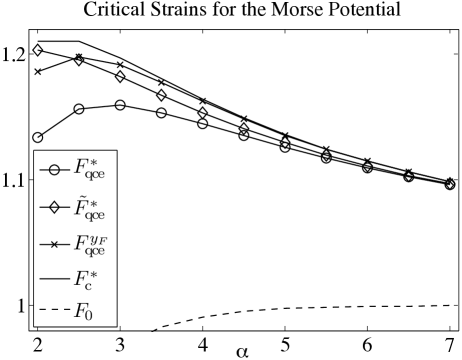
Figure 2. Critical strains $F_{\rm qce}^{*},\ \tilde{F}_{\rm qce}^{*},\ F_{\rm qce}^{y_{F}},\ F_{\rm c}^{*}$ and the equilibrium strain $F_{0}$, computed for the Morse potential (23) with varying $\alpha$. The critical strains for the QCE Hessian, $F_{\rm qce}^{*},$ are computed with $N=40$ and $K=10$. The approximation, $\tilde{F}_{\rm qce}^{*},$ is computed using the asymptotic approximation (25). The strain $F_{\rm qce}^{y_{F}}$ is the critical strain at which $\mathcal{E}_{\rm qce}^{\prime\prime}(y_{F})$ is no longer positive definite.

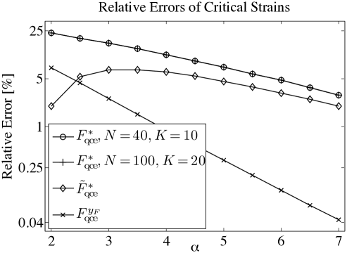
Figure 3. Relative errors of the critical strains (computed and predicted) for the QCE approximation against the critical strains of the QCL/QNL approximation. The errors are computed explicitly for $N=40,K=10$ as well as for $N=100,K=20$, using the Morse potential (23) with varying $\alpha$. These two curves are very close and may be hard to distinguish. Additionally, we show the critical strain for loss of positive definiteness of $\mathcal{E}_{\rm qce}^{\prime\prime}(y_{F}),$ which does not predict the loss of stability that the QCE experiences correctly for any parameter value.

We observe that the prediction for the critical strain, as well as the prediction for the relative error, obtained from our asymptotic analysis is insufficient for very soft potentials but becomes fairly accurate with increasing stiffness. In particular, it provides a good prediction of the relative errors for the critical strains for $\alpha\geq 3.5$.

For a correct interpretation of our results, we must first of all note that the relative errors for the critical strains decay exponentially with increasing stiffness $\alpha$. While, for small $\alpha$ (soft potentials) the error is quite severe, one could argue that it is insignificant (i.e., well below 10%) for moderately large $\alpha$ (stiff potentials). However, our point of view is that, by a careful choice of the atomistic region one should be able to control this error, as is the case for consistent QC approximations such as QNL. For the QCE approximation, this is impossible: the error in the critical strain is uncontrolled.

Conclusion

We propose sharp stability analysis as a theoretical criterion for evaluating the predictive capability of atomistic-to-continuum coupling methods. Our results show that a sharp stability analysis is as important as a sharp truncation error (consistency) analysis for the evaluation of atomistic-to-continuum coupling methods, and provides a new means to distinguish the relative merits of the various methods. Our results also provide an approach to establish a theoretical basis for the conclusions of the benchmark numerical tests reported in  [19], in particular for the poor performance of the QCE approximation in predicting the movement of a dipole of Lomer dislocations under applied shear.

Of course, the simple one-dimensional situation that we have considered here cannot nearly capture the complexity of atomistic-to-continuum coupling methods in 2D/3D. Even the much simpler question of whether QCL (the Cauchy-Born continuum model without coupling) can correctly predict bifurcation points becomes much more difficult since it is possible, in general, that the stability region for the Cauchy–Born model is much larger than that for atomistic model [10]. However, in many interesting situations this effect does not occur [13], and it is an interesting question to characterize these. Concerning the stability of the coupling mechanism, no rigorous results are available in 2D/3D. Until such an analysis is available, we propose that careful numerical experiments should be performed, which experimentally investigate the stability properties of atomistic-to-continuum coupling methods.

Appendix A Representations of $\mathcal{E}_{\rm qce}^{\prime}$ and $\mathcal{E}_{\rm qce}^{\prime\prime}$

Our aim in this section is to derive useful representations for the first and second variations $\mathcal{E}_{\rm qce}^{\prime}(y)$ and $\mathcal{E}_{\rm qce}^{\prime\prime}(y)$ of the QCE energy functional. For notational convenience, we will only write out terms in the right half of the domain $\{-N+1,\dots,N\}$, indicating the remaining terms (which can be obtained from symmetry considerations) by dots. For example, we write

$$\mathcal{E}_{\rm qce}(y)=~{} \dots+\varepsilon\sum_{\ell=0}^{N}\phi(y_{\ell}^{\prime})+\varepsilon\sum_{\ell=0}^{K-1}\phi(y_{\ell}^{\prime}+y_{\ell+1}^{\prime})+\varepsilon\sum_{\ell=K+2}^{N}\phi(2y_{\ell}^{\prime})$$

$$+{\textstyle\frac{\varepsilon}{2}}\phi(y_{K}^{\prime}+y_{K+1}^{\prime})+{\textstyle\frac{\varepsilon}{2}}\phi(y_{K+1}^{\prime}+y_{K+2}^{\prime})+{\textstyle\frac{\varepsilon}{2}}\phi(2y_{K+1}^{\prime}).$$

The first variation is a linear form on $\mathcal{U}$, given by

$$\mathcal{E}_{\rm qce}^{\prime}(y)[u]=\dots+\varepsilon\sum_{\ell=0}^{N}\phi^{\prime}(y_{\ell}^{\prime})u_{\ell}^{\prime}+\varepsilon\sum_{\ell=0}^{K-1}\phi^{\prime}(y_{\ell}^{\prime}+y_{\ell+1}^{\prime})(u_{\ell}^{\prime}+u_{\ell+1}^{\prime})$$

$$+{\textstyle\frac{\varepsilon}{2}}\phi^{\prime}(y_{K}^{\prime}+y_{K+1}^{\prime})(u_{K}^{\prime}+u_{K+1}^{\prime})+{\textstyle\frac{\varepsilon}{2}}\phi^{\prime}(y_{K+1}^{\prime}+y_{K+2}^{\prime})(u_{K+1}^{\prime}+u_{K+2}^{\prime})$$

$$+{\textstyle\frac{\varepsilon}{2}}\phi^{\prime}(2y_{K+1}^{\prime})(2u_{K+1}^{\prime})+\varepsilon\sum_{\ell=K+2}^{N}\phi^{\prime}(2y_{\ell}^{\prime})(2u_{\ell}^{\prime})$$ .

Collecting terms related to element strains $u_{\ell}^{\prime}$, we obtain

$$\begin{split}\mathcal{E}_{\rm qce}^{\prime}(y)[u]=\dots+\varepsilon\sum_{\ell=0}^{K-1}\big{\{}\phi^{\prime}(y_{\ell}^{\prime})+\phi^{\prime}(y_{\ell-1}^{\prime}+y_{\ell}^{\prime})+\phi^{\prime}(y_{\ell}^{\prime}+y_{\ell+1}^{\prime})\big{\}}~{}&u_{\ell}^{\prime}\\ +\varepsilon\big{\{}\phi^{\prime}(y_{K}^{\prime})+\phi^{\prime}(y_{K-1}^{\prime}+y_{K}^{\prime})+{\textstyle\frac{1}{2}}\phi^{\prime}(y_{K}^{\prime}+y_{K+1}^{\prime})\big{\}}~{}&u_{K}^{\prime}\\ +\varepsilon\big{\{}\phi^{\prime}(y_{K+1}^{\prime})+{\textstyle\frac{1}{2}}\phi^{\prime}(y_{K}^{\prime}+y_{K+1}^{\prime})+{\textstyle\frac{1}{2}}\phi^{\prime}(y_{K+1}^{\prime}+y_{K+2}^{\prime})+\phi^{\prime}(2y_{K+1}^{\prime})\big{\}}~{}&u_{K+1}^{\prime}\\ +\varepsilon\big{\{}\phi^{\prime}(y_{K+2}^{\prime}+{\textstyle\frac{1}{2}}\phi^{\prime}(y_{K+1}^{\prime}+y_{K+2}^{\prime})+2\phi^{\prime}(2y_{K+2}^{\prime})\big{\}}~{}&u_{K+2}^{\prime}\\ +\varepsilon\sum_{\ell=K+3}^{N}\big{\{}\phi^{\prime}(y_{\ell}^{\prime})+2\phi^{\prime}(2y_{\ell}^{\prime})\big{\}}~{}&u_{\ell}^{\prime}.\end{split}$$ (26)

Similarly, the second variation can be written in the form

$$\begin{split}\mathcal{E}_{\rm qce}^{\prime\prime}(y)[u,u]=\dots+\varepsilon\sum_{\ell=0}^{N}\phi^{\prime\prime}(y_{\ell}^{\prime})|u_{\ell}^{\prime}|^{2}+\varepsilon\sum_{\ell=0}^{K-1}\phi^{\prime\prime}(y_{\ell}^{\prime}+y_{\ell+1}^{\prime})|u_{\ell}^{\prime}+u_{\ell+1}^{\prime}|^{2}&\\ +{\textstyle\frac{\varepsilon}{2}}\phi^{\prime\prime}(y_{K}^{\prime}+y_{K+1}^{\prime})|u_{K}^{\prime}+u_{K+1}^{\prime}|^{2}+{\textstyle\frac{\varepsilon}{2}}\phi^{\prime\prime}(y_{K+1}^{\prime}+y_{K+2}^{\prime})|u_{K+1}^{\prime}+u_{K+2}^{\prime}|^{2}&\\ +{\textstyle\frac{\varepsilon}{2}}\phi^{\prime\prime}(2y_{K+1}^{\prime})|2u_{K+1}^{\prime}|^{2}+\varepsilon\sum_{\ell=K+2}^{N}\phi^{\prime\prime}(2y_{\ell}^{\prime})|2u_{\ell}^{\prime}|^{2}&.\end{split}$$ (27)

Using (8) to replace all second-neighbour terms in (27), we obtain the alternative representation

$$\mathcal{E}_{\rm qce}^{\prime\prime}(y)[u,u]=\dots+\varepsilon\sum_{\ell=0}^{K-1}\big{[}\phi^{\prime\prime}(y_{\ell}^{\prime})+2\phi^{\prime\prime}(y_{\ell-1}^{\prime}+y_{\ell}^{\prime})+2\phi^{\prime\prime}(y_{\ell}^{\prime}+y_{\ell+1}^{\prime})\big{]} |u_{\ell}^{\prime}|^{2}$$ (28)

$$+\varepsilon\big{[}\phi^{\prime\prime}(y_{K}^{\prime})+2\phi^{\prime\prime}(y_{K-1}^{\prime}+y_{K}^{\prime})+\phi^{\prime\prime}(y_{K}^{\prime}+y_{K+1}^{\prime})\big{]} |u_{K}^{\prime}|^{2}$$

$$+\varepsilon\big{[}\phi^{\prime\prime}(y_{K+1}^{\prime})+\phi^{\prime\prime}(y_{K}^{\prime}+y_{K+1}^{\prime})+\phi^{\prime\prime}(y_{K+1}^{\prime}+y_{K+2}^{\prime})+2\phi^{\prime\prime}(2y_{K+1}^{\prime})\big{]} |u_{K+1}^{\prime}|^{2}$$

$$+\varepsilon\big{[}\phi^{\prime\prime}(y_{K+2}^{\prime})+\phi^{\prime\prime}(y_{K+1}^{\prime}+y_{K+2}^{\prime})+4\phi^{\prime\prime}(2y_{K+2}^{\prime})\big{]} |u_{K+2}^{\prime}|^{2}$$

$$+\varepsilon\sum_{\ell=K+3}^{N}\big{[}\phi^{\prime\prime}(y_{\ell}^{\prime})+4\phi^{\prime\prime}(2y_{\ell}^{\prime})\big{]} |u_{\ell}^{\prime}|^{2}$$

$$-\varepsilon^{3}\sum_{\ell=0}^{K-1}\phi^{\prime\prime}(y_{\ell}^{\prime}+u_{\ell+1}^{\prime})|u_{\ell}^{\prime\prime}|^{2}-{\textstyle\frac{1}{2}}\varepsilon^{3}\big{\{}\phi^{\prime\prime}(y_{K}^{\prime}+y_{K+1}^{\prime})|u_{K}^{\prime\prime}|^{2}+\phi^{\prime\prime}(y_{K+1}^{\prime}+y_{K+2}^{\prime})|u_{K+1}^{\prime\prime}|^{2}\big{\}}.$$

While somewhat unwieldy at first glance, this representation is particularly useful for the stability analysis in Section 5.

Appendix B Proof of Lemma 5

In this section, we complete the proof of Lemma 5 which was merely hinted at in the main text of Section 5. Recall that $\hat{y}_{{\rm qce},F}=y_{F}+\delta_{1}\hat{g}$ where $\hat{g}$ is given by (13), and recall, moreover, that $\hat{y}_{\rm qce}$ solves the linear system

$$\phi_{F}^{\prime\prime}\langle(\hat{y}_{{\rm qce},F}-y_{F})^{\prime},u^{\prime}\rangle=\phi_{2F}^{\prime}\langle\hat{g}^{\prime},u^{\prime}\rangle=-\mathcal{E}_{\rm qce}^{\prime}(y_{F})[u]\qquad\text{ for all }u\in\mathcal{U}.$$ (29)

Our strategy is to prove that $\hat{y}_{{\rm qce},F}$ has a residual of order O($\delta_{1}^{2}+\delta_{1}\delta_{2}$) and that $\mathcal{E}_{\rm qce}^{\prime\prime}(\hat{y}_{{\rm qce},F})$ is an isomorphism between suitable function spaces. We will then apply a quantitative inverse function theorem to prove the existence of a solution $y_{{\rm qce},F}$ of the QCE criticality condition (11) which is “close” to $\hat{y}_{{\rm qce},F}$. Before we embark on this analysis, we make several comments and introduce some notation that will be helpful later on.

To ensure that $\mathcal{E}_{\rm qce}$ is sufficiently differentiable in a neighbourhood of $\hat{y}_{{\rm qce},F}$ we only need to assume that $F>0$ and that $\delta_{1}$ is sufficiently small, e.g., $\delta_{1}\leq F$. In that case, $\mathcal{E}_{\rm qce}$ is three times differentiable at $y$ for any $y\in\mathcal{Y}_{F}$ such that $\|y^{\prime}-\hat{y}_{{\rm qce},F}^{\prime}\|_{\ell^{\infty}}<{\textstyle\frac{1}{2}}\delta_{1}$.

We will interpret $\mathcal{E}_{\rm qce}^{\prime}$ as a nonlinear operator from $\mathcal{U}^{1,\infty}$ to $\mathcal{U}^{-1,\infty}$ which are, respectively, the spaces $\mathcal{U}$ and $\mathcal{U}^{*}$ endowed with the Sobolev-type norms,

$$\|u\|_{\mathcal{U}^{1,\infty}}=\|u^{\prime}\|_{\ell^{\infty}}\quad\text{for }u\in\mathcal{U},\quad\text{and}\quad\|T\|_{\mathcal{U}^{-1,\infty}}=\sup_{\begin{subarray}{c}v\in\mathcal{U}\\ \|v^{\prime}\|_{\ell^{1}_{\varepsilon}}=1\end{subarray}}T[v]\quad\text{for }T\in\mathcal{U}^{*}.$$

Consequently, for $y\in\mathcal{Y}_{F}$, $\mathcal{E}_{\rm qce}^{\prime\prime}(y)$ can be understood as a linear operator from $\mathcal{U}^{1,\infty}$ to $\mathcal{U}^{-1,\infty}$.

Our justification for defining $\hat{y}_{{\rm qce},F}$ as we did in (29) is the bound

$$\big{|}\mathcal{E}_{\rm qce}^{\prime\prime}(y_{F})[u,v]-\phi_{F}^{\prime\prime}\langle u^{\prime},v^{\prime}\rangle\big{|}\leq\phi_{F}^{\prime\prime}c_{1}\delta_{2}\|u^{\prime}\|_{\ell^{\infty}_{\varepsilon}}\|v^{\prime}\|_{\ell^{1}_{\varepsilon}}\quad\text{ for all }u,v\in\mathcal{U},$$ (30)

where $c_{1}=5$, which follows from (15). We can formulate this bound equivalently as

$$\|\mathcal{E}_{\rm qce}^{\prime\prime}(y_{F})-\phi_{F}^{\prime\prime}L_{1}\|_{L(\mathcal{U}^{1,\infty},\ \mathcal{U}^{-1,\infty})}\leq\phi_{F}^{\prime\prime}c_{1}\delta_{2},$$ (31)

where $L_{1}:\mathcal{U}\to\mathcal{U}^{*}$ is given by

$$L_{1}(u)[v]=\langle u^{\prime},v^{\prime}\rangle\qquad\text{ for all }u,v\in\mathcal{U}.$$

We also remark that $L_{1}:\mathcal{U}^{1,\infty}\to\mathcal{U}^{-1,\infty}$ is an isomorphism, uniformly bounded in $N$, more precisely,

$$\|L_{1}^{-1}\|_{L(\mathcal{U}^{-1,\infty},\ \mathcal{U}^{1,\infty})}\leq 2.$$ (32)

This result follows, for example, as a special case of [23, Eq. (36)] or [7, Eq. (5.2)], and is also contained in [6].

We are now ready to estimate the residual of $\hat{y}_{{\rm qce},F}$. Expanding $\mathcal{E}_{\rm qce}^{\prime}(\hat{y}_{{\rm qce},F})$ to first order gives

$$\begin{split}\mathcal{E}_{\rm qce}^{\prime}(\hat{y}_{{\rm qce},F})[v]=~{}&\big{\{}\mathcal{E}_{\rm qce}^{\prime}(y_{F})[v]+\delta_{1}\mathcal{E}_{\rm qce}^{\prime\prime}(y_{F})[\hat{g},v]\big{\}}\\ &+\delta_{1}\int_{0}^{1}\big{\{}\mathcal{E}_{\rm qce}^{\prime\prime}(y_{F}+t\delta_{1}\hat{g})[\hat{g},v]-\mathcal{E}_{\rm qce}^{\prime\prime}(y_{F})[\hat{g},v]\big{\}}\,{\rm d}t.\end{split}$$ (33)

We will estimate the two groups on the right-hand side of (33) separately. Using (12) and (30), we obtain

$$\begin{split}\big{|}\mathcal{E}_{\rm qce}^{\prime}(y_{F})[v]+\delta_{1}\mathcal{E}_{\rm qce}^{\prime\prime}(y_{F})[\hat{g},v]\big{|}=~{}&\delta_{1}\big{|}-\phi_{F}^{\prime\prime}\langle\hat{g}^{\prime},v^{\prime}\rangle+\mathcal{E}_{\rm qce}^{\prime\prime}(y_{F})[\hat{g},v]\big{|}\\ \leq~{}&\phi_{F}^{\prime\prime}c_{1}\delta_{1}\delta_{2}\|\hat{g}^{\prime}\|_{\ell^{\infty}_{\varepsilon}}\|v^{\prime}\|_{\ell^{1}_{\varepsilon}}\qquad\text{ for all }v\in\mathcal{U}.\end{split}$$ (34)

To estimate the second group in (33) we simply use the regularity of the interaction potential (we assumed that $\phi\in{\rm C}^{3}(0,+\infty)$) and Hölder’s inequality to obtain

$$\big{|}\mathcal{E}_{\rm qce}^{\prime\prime}(y_{F}+t\delta_{1}\hat{g})[\hat{g},v]-\mathcal{E}_{\rm qce}^{\prime\prime}(y_{F})[\hat{g},v]\big{|}\leq\phi_{F}^{\prime\prime}c_{2}t\delta_{1}\|\hat{g}^{\prime}\|_{\ell^{\infty}}^{2}\|v^{\prime}\|_{\ell^{1}_{\varepsilon}},$$ (35)

where $(\phi_{F}^{\prime\prime}c_{2})$ is a local Lipschitz constant for $\phi^{\prime\prime}$, that is, there exists a universal constant $\hat{c}_{2}$ such that

$$c_{2}=\hat{c}_{2}\sup_{|r|\leq{\textstyle\frac{1}{2}}\delta_{1}}\frac{\max(|\phi^{\prime\prime\prime}(F+r)|,|\phi^{\prime\prime\prime}(2(F+r))|)}{\phi_{F}^{\prime\prime}}.$$

In particular, if $\delta_{1}$ is sufficiently small then we may assume that

$$c_{2}=2\hat{c}_{2}\frac{\max(|\phi_{F}^{\prime\prime\prime}|,|\phi_{2F}^{\prime\prime\prime}|)}{\phi_{F}^{\prime\prime}}.$$

Inserting (35) and (34) into (33), and using the fact that $\|\hat{g}^{\prime}\|_{\ell^{\infty}}={\textstyle\frac{1}{2}}$, we obtain the $\mathcal{U}^{-1,\infty}$-residual estimate

$$\|\mathcal{E}_{\rm qce}^{\prime}(\hat{y}_{{\rm qce},F})\|_{\mathcal{U}^{-1,\infty}}\leq\phi_{F}^{\prime\prime}({\textstyle\frac{1}{2}}c_{1}\delta_{1}\delta_{2}+{\textstyle\frac{1}{8}}c_{2}\delta_{1}^{2}).$$

Next, we estimate $\|\mathcal{E}_{\rm qce}^{\prime\prime}(\hat{y}_{{\rm qce},F})^{-1}\|_{L(\mathcal{U}^{-1,\infty},\ \mathcal{U}^{1,\infty})}$. Using (31) and a similar argument as for (35) gives

$$\|\mathcal{E}_{\rm qce}^{\prime\prime}(\hat{y}_{{\rm qce},F})-\phi_{F}^{\prime\prime}L_{1}\|_{L(\mathcal{U}^{1,\infty},\ \mathcal{U}^{-1\infty})}\leq~{} \|\mathcal{E}_{\rm qce}^{\prime\prime}(\hat{y}_{{\rm qce},F})-\mathcal{E}_{\rm qce}^{\prime\prime}(y_{F})\|_{L(\mathcal{U}^{1,\infty},\ \mathcal{U}^{-1\infty})}$$

$$+\|\mathcal{E}_{\rm qce}^{\prime\prime}(y_{F})-\phi_{F}^{\prime\prime}L_{1}\|_{L(\mathcal{U}^{1,\infty},\ \mathcal{U}^{-1\infty})}$$

$$\leq~{} \phi_{F}^{\prime\prime}({\textstyle\frac{1}{2}}c_{2}\delta_{1}+c_{1}\delta_{2}).$$

Moreover, from (32), we deduce that

$$\|(\phi_{F}^{\prime\prime}L_{1})^{-1}\|_{L(\mathcal{U}^{-1,\infty},\ \mathcal{U}^{1,\infty})}\leq\frac{2}{\phi_{F}^{\prime\prime}}.$$

A standard result of operator theory states that if $X,Y$ are Banach spaces and $T,S:X\to Y$ are bounded linear operators with $T$ being invertible and satisfying $\|S-T\|<1/\|T^{-1}\|,$ then $S$ is invertible and

$$\|S^{-1}\|\leq\frac{\|T^{-1}\|}{1-\|T^{-1}\|\|S-T\|}.$$

In our case, setting $T=\phi_{F}^{\prime\prime}L_{1}$ and $S=\mathcal{E}_{\rm qce}^{\prime\prime}(\hat{y}_{{\rm qce},F})$, this translates to

$$\|\mathcal{E}_{\rm qce}^{\prime\prime}(\hat{y}_{{\rm qce},F})^{-1}\|_{L(\mathcal{U}^{-1,\infty},\ \mathcal{U}^{1,\infty})}\leq\frac{2}{\phi_{F}^{\prime\prime}(1-{\textstyle\frac{1}{2}}c_{2}\delta_{1}-c_{1}\delta_{2})},$$

provided that the denominator is positive. Thus, for $\delta_{1},\delta_{2}$ sufficiently small, we obtain the bound

$$\|\mathcal{E}_{\rm qce}^{\prime\prime}(\hat{y}_{{\rm qce},F})^{-1}\|_{L(\mathcal{U}^{-1,\infty},\ \mathcal{U}^{1,\infty})}\leq\frac{4}{\phi_{F}^{\prime\prime}}.$$

We now apply the following version of the inverse function theorem.

Lemma 7. Let $X,Y$ be Banach spaces, $U$ an open subset of $X$, and let $F:U\to Y$ be Fréchet differentiable. Suppose that $x_{0}\in U$ satisfies the conditions

$$\|F(x_{0})\|_{Y}\leq\eta,\quad\|F^{\prime}(x_{0})^{-1}\|_{L(Y,X)}\leq\sigma^{-1},$$

$$\overline{B_{X}(x_{0},2\eta\sigma^{-1})}\subset U,$$

$$\|F^{\prime}(x_{1})-F^{\prime}(x_{2})\|_{L(X,Y)}\leq L\|x_{1}-x_{2}\|_{X}\quad\text{for}\quad\|x_{j}-x_{0}\|_{X}\leq 2\eta\sigma^{-1},$$

$$\text{ and }2L\sigma^{-2}\eta<1,$$

then there exists $x\in X$ such that $F(x)=0$ and $\|x-x_{0}\|_{X}\leq 2\eta\sigma^{-1}$.

Proof.

The result follows, for example, by applying Theorem 2.1 in [22] with the choices $R=2\eta\sigma^{-1}$, $\omega(x_{0},R)=LR$ and $\bar{\omega}(x_{0},R)=\frac{1}{2}LR^{2}$. Similar results can be obtained by tracking the constants in most proofs of the inverse function theorem, and assuming local Lipschitz continuity of $F^{\prime}$. ∎

For our purposes, we set $X=\mathcal{U}^{1,\infty}$, $Y=\mathcal{U}^{-1,\infty}$, $F(u)=\mathcal{E}_{\rm qce}^{\prime}(\hat{y}_{{\rm qce},F}+u)$, and $x_{0}=0$. Assuming that $\delta_{1},\delta_{2}$ are sufficiently small, our previous analysis gives the residual and stability estimates

$$\eta=\phi_{F}^{\prime\prime}({\textstyle\frac{1}{2}}c_{1}\delta_{1}\delta_{2}+{\textstyle\frac{1}{8}}c_{2}\delta_{1}^{2})\quad\text{and}\quad\sigma={\textstyle\frac{1}{4}}\phi_{F}^{\prime\prime},$$

and, in particular,

$$2\eta\sigma^{-1}=4c_{1}\delta_{1}\delta_{2}+c_{2}\delta_{1}^{2}.$$

To ensure that $\overline{B_{\mathcal{U}^{1,\infty}}(0,2\eta\sigma^{-1})}$ remains within the region of differentiability of $F$, that is, to ensure that $(\hat{y}_{{\rm qce},F}+u)_{\ell}^{\prime}>0$ for $\|u^{\prime}\|_{\ell^{\infty}}\leq 2\eta\sigma^{-1}$, it is clearly enough to assume that $\delta_{1}$ and $\delta_{2}$ are sufficiently small.

A modification of (35) then allows the choice $L=2\phi_{F}^{\prime\prime}c_{2}$ for the local Lipschitz constant.

Thus, the condition ensuring the existence of a solution $y_{{\rm qce},F}$ of (11) becomes

$$4L\sigma^{-2}\eta=64c_{1}c_{2}\delta_{1}\delta_{2}+16c_{2}^{2}\delta_{1}^{2}<1,$$

which is satisfied, once again, if we assume that $\delta_{1}$ and $\delta_{2}$ are sufficiently small. An application of Lemma B concludes the proof of Lemma 5.

References

- [1] S. Badia, M. L. Parks, P. B. Bochev, M. Gunzburger, and R. B. Lehoucq. On atomistic-to-continuum coupling by blending. SIAM J. Multiscale Modeling & Simulation, 7(1):381–406, 2008.
- [2] X. Blanc, C. Le Bris, and F. Legoll. Analysis of a prototypical multiscale method coupling atomistic and continuum mechanics. M2AN Math. Model. Numer. Anal., 39(4):797–826, 2005.
- [3] M. Dobson and M. Luskin. Analysis of a force-based quasicontinuum approximation. M2AN Math. Model. Numer. Anal., 42(1):113–139, 2008.
- [4] M. Dobson and M. Luskin. An analysis of the effect of ghost force oscillation on the quasicontinuum error. Mathematical Modelling and Numerical Analysis, 43:591–604, 2009.
- [5] M. Dobson and M. Luskin. An optimal order error analysis of the one-dimensional quasicontinuum approximation. SIAM. J. Numer. Anal., 47:2455–2475, 2009.
- [6] M. Dobson, M. Luskin, and C. Ortner. Sharp stability estimates for force-based quasicontinuum approximation of homogeneous tensile deformation. Multiscale Modeling and Simulation, to appear.
- [7] M. Dobson, M. Luskin, and C. Ortner. Stability, instability, and error of the force-based quasicontinuum approximation. Arch. Rat. Mech. Anal., to appear.
- [8] W. E, J. Lu, and J. Yang. Uniform accuracy of the quasicontinuum method. Phys. Rev. B, 74(21):214115, 2004.
- [9] W. E and P. Ming. Analysis of the local quasicontinuum method. In Frontiers and prospects of contemporary applied mathematics, volume 6 of Ser. Contemp. Appl. Math. CAM, pages 18–32. Higher Ed. Press, Beijing, 2005.
- [10] W. E and P. Ming. Cauchy-Born rule and the stability of crystalline solids: static problems. Arch. Ration. Mech. Anal., 183(2):241–297, 2007.
- [11] M. Gunzburger and Y. Zhang. A quadrature-rule type approximation for the quasicontinuum method. manuscript, 2008.
- [12] M. Gunzburger and Y. Zhang. Quadrature-rule type approximations to the quasicontinuum method for short and long-range interatomic interactions. manuscript, 2008.
- [13] T. Hudson and C. Ortner. On the stability of atomistic models and their cauchy–born approximations. in preparation.
- [14] P. Lin. Theoretical and numerical analysis for the quasi-continuum approximation of a material particle model. Math. Comp., 72(242):657–675, 2003.
- [15] P. Lin. Convergence analysis of a quasi-continuum approximation for a two-dimensional material without defects. SIAM J. Numer. Anal., 45(1):313–332 (electronic), 2007.
- [16] M. Luskin and C. Ortner. An analysis of node-based cluster summation rules in the quasicontinuum method. SIAM J. Numer. Anal., 47(4):3070–3086, 2009.
- [17] D. M, M. Luskin, and C. Ortner. Iterative methods for the force-based quasicontinuum approximation. arXiv:0910.2013.
- [18] R. Miller and E. Tadmor. The Quasicontinuum Method: Overview, Applications and Current Directions. Journal of Computer-Aided Materials Design, 9:203–239, 2003.
- [19] R. Miller and E. Tadmor. Benchmarking multiscale methods. Modelling and Simulation in Materials Science and Engineering, 17:053001 (51pp), 2009.
- [20] P. Ming and J. Z. Yang. Analysis of a one-dimensional nonlocal quasi-continuum method. Multiscale Model. Simul., 7(4):1838–1875, 2009.
- [21] M. Ortiz, R. Phillips, and E. B. Tadmor. Quasicontinuum Analysis of Defects in Solids. Philosophical Magazine A, 73(6):1529–1563, 1996.
- [22] C. Ortner. A posteriori existence in numerical computations. SIAM J. Numer. Anal., 47(4):2550–2577, 2009.
- [23] C. Ortner and E. Süli. Analysis of a quasicontinuum method in one dimension. M2AN Math. Model. Numer. Anal., 42(1):57–91, 2008.
- [24] S. Prudhomme, P. T. Bauman, and J. T. Oden. Error control for molecular statics problems. International Journal for Multiscale Computational Engineering, 4(5-6):647–662, 2006.
- [25] V. B. Shenoy, R. Miller, E. B. Tadmor, D. Rodney, R. Phillips, and M. Ortiz. An adaptive finite element approach to atomic-scale mechanics–the quasicontinuum method. J. Mech. Phys. Solids, 47(3):611–642, 1999.
- [26] T. Shimokawa, J. Mortensen, J. Schiotz, and K. Jacobsen. Matching conditions in the quasicontinuum method: Removal of the error introduced at the interface between the coarse-grained and fully atomistic region. Phys. Rev. B, 69(21):214104, 2004.
- [27] E. Süli and D. F. Mayers. An introduction to numerical analysis. Cambridge University Press, Cambridge, 2003.