Plasma cutoff and enhancement of radiative transitions in dense stellar matter

Abstract

We study plasma effects on radiative transitions (e.g., decay of excited states of atoms or atomic nuclei) in a dense plasma at the transition frequencies $\omega\lesssim\omega_{p}$ (where $\omega_{p}$ is the electron plasma frequency). The decay goes through four channels – the emission of real transverse and longitudinal plasmons as well as the emission of virtual transverse and longitudinal plasmons with subsequent absorption of such plasmons by the plasma. The emission of real plasmons dies out at $\omega\leq\omega_{p}$, but the processes with virtual plasmons strongly enhance the radiative decay. Applications of these results to radiative processes in white dwarf cores and neutron star envelopes are discussed.

I Introduction

Radiative processes in stars are very important. First of all, they determine heat transport in radiative zones of the stars Cox and Giuli (1968), as well as the radiative transfer and structure of stellar atmospheres together with the formation of spectra of stellar radiation Chandrasekhar (1960); Sobolev (1969). In ordinary stars (at the main sequence or around) typical radiation frequencies are much higher than the electron plasma frequency $\omega_{p}$ of stellar matter. As a result, plasma effects do not affect strongly radiative processes.

However, in a dense matter of compact stars (white dwarfs and neutron stars) the plasma frequency can be higher or comparable to characteristic radiation transition frequencies $\omega$, and the plasma effects cannot be ignored. For instance, in a strongly degenerate nonrelativistic electron gas at a density of $10^{3}$ g cm^-3 (that is typical for degenerate cores of white dwarfs and outer envelopes of neutron stars) one has $\hbar\omega_{p}\approx 0.6$ keV. In this example the plasma effects can easily affect radiative transitions in atoms and ions. In the inner crust of a neutron star at a density of $10^{12}$ g cm^-3, where the degenerate electrons are ultrarelativistic, the plasma frequency becomes very large, $\hbar\omega_{p}\sim 3$ MeV (depending on the composition of the crust; e.g., Ref. Haensel et al. (2007); also see Sec. VI). This is large enough to influence radiative transitions in atomic nuclei.

The importance of plasma effects for radiative processes in dense stellar matter has been mentioned in the literature (e.g., Ref. Buchler and Yueh (1976)). In particular, the plasma effects on the radiative thermal conductivity have been studied in Refs. Aharony and Opher (1979); Yu. K. Kurilenkov and Van Horn (1994) but these studies are not fully complete (Sec. VI). For another example, consider an emitter (an ion or atomic nucleus) in an excited state with the transition frequency $\omega$ to the ground state that is lower than $\omega_{p}$. What will happen with this emitter taking into account that radiative transitions with the emission of any electromagnetic quanta are now forbidden? Will it live at the excited level forever?

These questions can be answered using the available theory of electromagnetic transitions in a plasma. The plasma impact on electromagnetic transitions in an non-relativistic laboratory plasma and a rarefied non-relativistic cosmic plasma has been studied for a long time (e.g., Refs. Weisheit and Murillo (1998); Oiringel’ and Kleiman (1984)). The plasma effects can modify the emission of electromagnetic quanta Oiringel’ and Kleiman (1984). Moreover, collective plasma processes open another electromagnetic transition channel – the emission of virtual plasmons and successive absorbtion of these plasmons by the plasma Klimontovich (1983); Weisheit and Murillo (1998). The most pronounced of these effects seems to be collisional broadening of energy levels of atoms and ions and associated broadening of spectral lines. It can be important in cosmic and laboratory plasmas Klimontovich (1983).

To the best of our knowledge, the theory of radiative transitions in a plasma (e.g., Refs. Klimontovich (1983); Weisheit and Murillo (1998)) has been correctly applied only to study non-degenerate laboratory and cosmic plasmas. In this paper we investigate the radiative transitions in a dense degenerate relativistic electron gas, particularly at $\omega<\omega_{p}$. The paper is organized as follows. In Sec. II we outline the formalism for calculating electromagnetic transitions rates in a dense plasma. It is similar to the formalism of stopping power for a charged particle moving in a plasma Aleksandrov et al. (1984). In Sec. III we outline the main properties of a degenerate electron plasma. Section IV is devoted to the radiative decay in the plasma for those transitions that are allowed in the electric dipole approximation. In Sec. V we address similar problem for the electric quadrupole and magnetic dipole transitions. In Sec. VI we discuss the main results and some applications, particularly, for calculating radiative thermal conductivity in white dwarf cores and neutron star envelopes and for studying radiative decay of excited states of atomic nuclei and kinetics of neutrons in the neutron star crust. We conclude in Sec. VII.

II Four radiative transition channels

Let us consider an external emitter (for instance, an atom or atomic nucleus) immersed in a plasma. The plasma is assumed to be uniform and isotropic; it is characterized by the longitudinal and transverse dielectric functions $\varepsilon_{\mathrm{l}}(\omega,k)$ and $\varepsilon_{\mathrm{tr}}(\omega,k)$, respectively. We are interested in the transition rate $w_{i\to f}$ [s^-1] at zero temperature ($T=0$) from an upper state $i$ to a lower state $f$ whose energy separation is $\hbar\omega$. The expression for $w_{i\to f}$ can be written as Klimontovich (1983)

$$w_{i\to f}=-\frac{e^{2}}{\pi^{2}\hbar}\Im\int\limits_{0}^{\infty}{\rm d}k\int\limits_{(4\pi)}{\rm d}\Omega_{\bm{k}}\left[\frac{\left|\bm{j}_{fi}(\bm{k})\bm{\cdot}\bm{k}\right|^{2}}{\omega^{2}\varepsilon_{\mathrm{l}}(\omega,k)}+\frac{\left|\bm{j}_{fi}(\bm{k})\bm{\times}\bm{k}\right|^{2}}{\omega^{2}\varepsilon_{\mathrm{tr}}(\omega,k)-k^{2}c^{2}}\right].$$ (1)

Any elementary transition (characterized by the given energy loss $\hbar\omega$) is accompanied by the transfer of an elementary excitation with a wavevector $\bm{k}$ to a plasma coupled to electromagnetic field. The integration is performed over all allowed values of $\bm{k}$ (with $k=|\bm{k}|$, and d$\Omega_{\bm{k}}$ being a solid angle element in the direction of $\bm{k}$). Furthermore,

$$\bm{j}_{fi}(\bm{k})=\int{\rm d}V\,\bm{j}_{fi}(\bm{r})\exp(-i\bm{k}\bm{r})$$ (2)

is the Fourier transform of the local transition current $\bm{j}_{fi}(\bm{r})$ Berestetskii et al. (1984). The latter current can be calculated from relativistic theory with stationary (relativistic) wave functions of the emitter in the $i$ and $f$ states. The transition rate (1) is cumulative. It includes contributions of transition channels with different $\bm{k}$ and different structures of plasma-electromagnetic field excitations. Particularly, it intrinsically contains a sum over polarizations of emitted plasmons (see below). It neglects the contribution of two- and multiple-plasmon processes which is expected to be small in the cumulative rate.

The dielectric functions (with spatial dispersion) in Eq. (1) take into account the plasma effects on the transition rate Weisheit and Murillo (1998); Klimontovich (1983). In particular, Eq. (1) includes the contribution of direct interaction of the emitter with plasma electrons.

The transition rate (1) can be decomposed as (Table 1)

$$w_{i\to f}=w_{i\to f}^{\mathrm{l}}+w_{i\to f}^{\mathrm{tr}}=w_{i\to f}^{\mathrm{Al}}+w_{i\to f}^{\mathrm{Bl}}+w_{i\to f}^{\mathrm{Atr}}+w_{i\to f}^{\mathrm{Btr}}.$$ (3)

Here, $w_{i\to f}^{\mathrm{l}}$ and $w_{i\to f}^{\mathrm{tr}}$ correspond to the longitudinal and transverse channels [the terms in (1) containing $\varepsilon_{\mathrm{l}}(\omega,k)$ and $\varepsilon_{\mathrm{tr}}(\omega,k)$, respectively]. Each of these terms, in turn, contains two contributions – (A) the emission of a real longitudinal (Al) or transverse (Atr) plasmon and (B) the emission and absorption of a virtual longitudinal (Bl) or transverse (Btr) plasmon. Not all of the four channels can be opened at once (see below).

Table 1: Four transition channels in plasma environment.

Channel	Plasmon	Open at	Comment
Atr	real transverse	$\omega_{p}<\omega$	Dominates at $\omega\gtrsim\omega_{p}$
Al	real longitudinal	$0<\omega-\omega_{p}\lesssim\omega_{p}$
Btr	virtual transverse	any $\omega$
Bl	virtual longitudinal	any $\omega$	Dominates at $\omega\lesssim\omega_{p}$

The emission of real plasmons (channels Al and Atr) is allowed in the presence of the poles in the denominators of Eq. (1), that is at

$$\varepsilon_{\mathrm{l}}(\omega,k)=0,\quad\omega^{2}\varepsilon_{\mathrm{tr}}(\omega,k)=k^{2}c^{2}.$$ (4)

The roots of these equations give the plasmon dispersion relations $k_{\mathrm{l}}(\omega)$ and $k_{\mathrm{tr}}(\omega)$ for longitudinal and transverse plasmons, respectively. The emission rates for real longitudinal and transverse plasmons are then given by the standard expressions Oiringel’ and Kleiman (1984)

$$w_{i\to f}^{\mathrm{Al}} = \frac{e^{2}}{\pi\hbar\omega^{2}}\int\limits_{(4\pi)}{\rm d}\Omega_{\bm{k}}\left|\bm{j}_{fi}(\bm{k})\bm{\cdot}\bm{k}\right|^{2}\left|\frac{\partial\varepsilon_{\mathrm{l}}(\omega,k)}{\partial k}\right|^{-1}_{~{}k=k_{\mathrm{l}}(\omega)},$$ (5)

$$w_{i\to f}^{\mathrm{Atr}} = \frac{e^{2}}{\pi\hbar}\int\limits_{(4\pi)}{\rm d}\Omega_{\bm{k}}\left|\bm{j}_{fi}(\bm{k})\bm{\times}\bm{k}\right|^{2}\left|\frac{\partial\left[\omega^{2}\varepsilon_{\mathrm{tr}}(\omega,k)-k^{2}c^{2}\right]}{\partial k}\right|^{-1}_{~{}k=k_{\mathrm{tr}}(\omega)}.$$ (6)

In principle, there can be several poles for one $\omega$; then one should sum over the poles in these equations.

The processes Bl and Btr in Eq. (1) involve virtual plasmons. These processes are allowed if the dielectric functions have imaginary parts for some values of $k$ at a given $\omega$. Nonvanishing imaginary parts of dielectric functions ensure that the plasma can directly absorb electromagnetic fluctuations induced by the emitter. From Eq. (1) one has Klimontovich (1983)

$$w_{i\to f}^{\mathrm{Bl}} = \frac{e^{2}}{\pi^{2}\hbar\omega^{2}}\int\limits_{0}^{\infty}{\rm d}k\int\limits_{(4\pi)}{\rm d}\Omega_{\bm{k}}\,\frac{\left|\bm{j}_{fi}(\bm{k})\bm{\cdot}\bm{k}\right|^{2}\Im\varepsilon_{\mathrm{l}}(\omega,k)}{\left|\varepsilon_{\mathrm{l}}(\omega,k)\right|^{2}},$$ (7)

$$w_{i\to f}^{\mathrm{Btr}} = \frac{e^{2}\omega^{2}}{\pi^{2}\hbar}\int\limits_{0}^{\infty}{\rm d}k\int\limits_{(4\pi)}{\rm d}\Omega_{\bm{k}}\,\frac{\left|\bm{j}_{fi}(\bm{k})\bm{\times}\bm{k}\right|^{2}\Im\varepsilon_{\mathrm{tr}}(\omega,k)}{\left|\omega^{2}\varepsilon_{\mathrm{tr}}(\omega,k)-k^{2}c^{2}\right|^{2}}.$$ (8)

Virtual plasmons do not obey any specific dispersion relation and can have a wide spectrum of wavenumbers $k$ for a given $\omega$. Equations (7) and (8) describe the effects which are in common with collisional broadening of spectral lines (and associated enhancement of radiative transition rates) in atomic physics Klimontovich (1983).

Equations (5)–(8) can be used to study radiative transition rates of a relativistic emitter in any uniform and isotropic dispersive medium (we set $T\to 0$ and disregard thus induced transitions).

In vacuum, where $\varepsilon_{\mathrm{l}}=\varepsilon_{\mathrm{tr}}\equiv 1$, only one channel survives out of the four. It is Atr – the emission of real transverse plasmons, and these plasmons become identical to ordinary photons. Then Eq. (6) reduces to the well known expression Berestetskii et al. (1984)

$$w_{i\to f}^{\mathrm{Atr}}\equiv w_{i\to f}^{\mathrm{vac}}=\frac{e^{2}\omega}{2\pi\hbar c^{3}}\int\limits_{(4\pi)}{\rm d}\Omega_{\bm{k}}\left|\bm{j}_{fi}(\bm{k})\bm{\times}\bm{\hat{k}}\right|^{2},$$ (9)

where $\bm{\hat{k}}=\bm{k}/k$.

Let us stress that the existence of the four radiative decay channels and general expressions for the partial decay rates have been known long ago (e.g., Refs. Klimontovich (1983); Oiringel’ and Kleiman (1984)). However, this formalism has been mostly applied to radiative transitions in a non-degenerate plasma, where radiation frequencies are typically much higher than $\omega_{p}$. In this case the exchange of virtual plasmons is usually unimportant, and the authors focused on the emission of real plasmons that was not strongly affected by the plasma environment. We will apply the above formalism to analyze dense degenerate electron stellar matter where the plasma effects are pronounced much stronger.

III Plasma environment of degenerate electrons

Let us study plasma effects in a strongly degenerate (zero temperature) ideal electron gas of any degree of relativity in the absence of a magnetic field. We will comment on the effects of finite temperature, ion plasma polarization and magnetic fields in Sec. VI. We employ the collisionless dielectric functions $\varepsilon_{\mathrm{tr}}(\omega,k)$ and $\varepsilon_{\mathrm{l}}(\omega,k)$ of a relativistic electron gas at $T=0$ derived by Jancovici Jancovici (1962) in the random phase approximation. We do not present his cumbersome expressions here (note that they should be corrected Kantor and Gusakov (2007) at certain values of $\omega$ and $k$) but discuss their main properties relevant to our study.

The most important quantity is the electron plasma frequency,

$$\omega_{p}=\sqrt{4\pi e^{2}n_{e}/m_{e}^{\ast}},$$ (10)

where $n_{e}$ is the electron number density, $m_{e}^{\ast}=\mu_{e}/c^{2}$ is the effective electron mass on the Fermi surface, $\mu_{e}=\sqrt{m_{e}^{2}c^{4}+c^{2}p_{F}^{2}}$ the electron chemical potential (electron rest-mass energy included), $p_{F}=\hbar(3\pi^{2}n_{e})^{1/3}$ being the electron Fermi momentum. We also introduce the electron Fermi velocity $v_{F}=p_{F}/m_{e}^{\ast}$.

The functions $\varepsilon_{\mathrm{tr}}(\omega,k)$ and $\varepsilon_{\mathrm{l}}(\omega,k)$ are generally complex. Their real parts describe plasma effects on the propagation of electromagnetic fluctuations, while their imaginary parts describe dissipation of such fluctuations. Under typical parameters in dense stellar matter for the processes of our study (Sec. I), the main source of dissipation is provided by the Cherenkov-type absorption at $\omega\leq kv_{F}$ (e.g., Ref. Aleksandrov et al. (1984)). At $T=0$ the dissipation switches on abruptly in this domain; it is absent whenever $\omega>kv_{F}$. Thus the integration over $k$ in Eqs. (7) and (8) can be truncated at $k=\omega/v_{F}$. Furthermore, in dense stellar environment it is reasonable to assume that radiative transition energies are not too large, $\hbar\omega\ll v_{F}p_{F}$, and $\hbar\omega_{p}\ll v_{F}p_{F}$. This smallness of $\hbar\omega$ and $\hbar\omega_{p}$ with respect to typical electron energies greatly simplifies the consideration.

At $\omega\sim\omega_{p}$ and $k\ll\omega/v_{F}$ the dissipation effect is absent, and the dielectric functions take the form

$$\varepsilon_{\mathrm{l}}(\omega,k) \approx 1-\frac{\omega_{p}^{2}}{\omega^{2}}\left(1+\frac{3}{5}\;\frac{k^{2}v_{F}^{2}}{\omega^{2}}\right),$$ (11)

$$\varepsilon_{\mathrm{tr}}(\omega,k) \approx 1-\omega_{p}^{2}/\omega^{2}.$$ (12)

From Eqs. (4) and (12) we immediately obtain the dispersion relation for the transverse waves

$$\omega^{2}_{\mathrm{tr}}=\omega_{p}^{2}+c^{2}k^{2}.$$ (13)

This is a good approximation for all $k$. It corresponds to two transverse plasma modes with different polarizations, but the same dispersion relation. The wave frequency satisfies the inequality $\omega_{\mathrm{tr}}>kv_{F}$ at any $k$. Therefore, these waves undergo no collisionless damping. One has $\omega_{\mathrm{tr}}\to\omega_{p}$ as $k\to 0$; and $\omega_{\mathrm{tr}}\approx kc$ as $k\gg\omega_{p}/c$. In the latter case these waves turn into ordinary photons which are almost unaffected by the plasma environment.

From Eqs. (4) and (11) one can derive the dispersion relation for the longitudinal (electron Langmuir) plasma waves Aleksandrov et al. (1984),

$$\omega^{2}_{\mathrm{l}}=\omega_{p}^{2}+{3\over 5}\,v_{F}^{2}k^{2}.$$ (14)

This equation is valid at $k\ll\omega_{p}/v_{F}$, when $\omega_{\mathrm{l}}$ is only slightly higher than $\omega_{p}$, and the collisionless damping is absent. At higher $k$ the dispersion equation must be solved numerically. The solution shows that at some $\omega_{\mathrm{l}}$ ($\sim\omega_{p}$) the derivative $\partial\varepsilon_{\rm l}(\omega,k)/\partial k$ becomes very large. This means that the transition rate $w_{i\to f}^{\mathrm{Al}}$ switches off when the transition frequency $\omega$ exceeds some value (a few $\omega_{p}$).

It is important that the frequencies of longitudinal and transverse plasma waves are always higher than $\omega_{p}$. This implies that corresponding transition rates undergo the plasma frequency cutoff,

$$w_{i\to f}^{\mathrm{Atr}}=w_{i\to f}^{\mathrm{Al}}=0\quad\mathrm{at}~{}~{}\omega\leq\omega_{p}.$$ (15)

Finally, let us outline absorption properties of degenerate electron plasma. For typical conditions in dense stellar matter, there are two domains Jancovici (1962) in the $(\omega,k)$-plane, where the imaginary parts of the longitudinal and transverse dielectric functions are non-zero. The first domain is given by the inequality $\hbar\omega<\mu-E_{p_{F}-\hbar k}$ at $\hbar k<2p_{F}$; the second domain is determined by $|E_{p_{F}-\hbar k}-\mu|<\hbar\omega<E_{p_{F}+\hbar k}-\mu$ at any $k$, with $E_{p}=\sqrt{c^{2}p^{2}+m_{e}^{2}c^{4}}$. The analytic expressions for the imaginary parts of the dielectric functions in these two domains are different. Although we have used exact expressions in computations, we notice that in the ultrarelativistic gas it is sufficient to consider the only one domain $\omega/v_{F}\lesssim k\lesssim 2p_{F}/\hbar$, where, to a good approximation,

$$\Im\varepsilon_{\mathrm{l}} = \frac{3\pi\omega_{p}^{2}}{2\omega^{2}x^{3}}\left(1-\frac{x^{2}\hbar^{2}\omega^{2}}{4p_{F}^{2}c^{2}}\right),$$ (16)

$$\Im\varepsilon_{\mathrm{tr}} = \frac{3\pi\omega_{p}^{2}}{4\omega^{2}x^{3}}\left[x^{2}-1+\frac{x^{2}\hbar^{2}\omega^{2}}{4p_{F}^{2}c^{2}}\left({x^{2}c^{2}\over v_{F}^{2}}-1\right)\right],$$ (17)

with $x=kv_{F}/\omega$.

IV Electric dipole transitions

Let us calculate the transition rate $w_{i\to f}$ in the electric dipole approximation (E1). The approximation is valid at $ka\ll 1$, where $a$ is a typical size of the emitter, and $k$ a typical plasmon wavenumber. In this case, the transition current is independent of $\bm{k}$, $\bm{j}_{fi}(\bm{k})\approx\bm{j}_{fi}({\bm{0}})$. The angular integration gives

$$\int\limits_{(4\pi)}{\rm d}\Omega_{\bm{k}}\left|\bm{j}_{fi}(\bm{0})\bm{\cdot}\bm{k}\right|^{2} = \frac{4\pi}{3}\left|{\bm{j}}_{fi}({\bm{0}})\right|^{2}k^{2},$$ (18)

$$\int\limits_{(4\pi)}{\rm d}\Omega_{\bm{k}}\left|\bm{j}_{fi}(\bm{0})\bm{\times}\bm{k}\right|^{2} = \frac{8\pi}{3}\left|{\bm{j}}_{fi}({\bm{0}})\right|^{2}k^{2}.$$ (19)

Then the in-vacuum transition rate (associated with the emission of ordinary photons) is given by the standard expression Berestetskii et al. (1984)

$$w_{i\to f}^{\mathrm{vac}}=\frac{4e^{2}\omega\left|\bm{j}_{fi}(\bm{0})\right|^{2}}{3\hbar c^{3}}=\frac{4e^{2}\omega^{3}}{3\hbar c^{3}}\left|\bm{r}_{fi}\right|^{2},$$ (20)

where we have used the relation $\bm{j}_{fi}(\bm{0})\approx-i\omega\bm{r}_{fi}$, $\bm{r}_{fi}$ being the position-vector matrix element.

It is convenient to rewrite Eq. (3) as

$$w_{i\to f}=w_{i\to f}^{\mathrm{vac}}R=w_{i\to f}^{\mathrm{vac}}\left(R_{\mathrm{Al}}+R_{\mathrm{Bl}}+R_{\mathrm{Atr}}+R_{\mathrm{Btr}}\right),$$ (21)

where $R_{\mathrm{Al}}$, $R_{\mathrm{Bl}}$, $R_{\mathrm{Atr}}$, and $R_{\mathrm{Btr}}$ are the factors, which describe the plasma effects on the transition rates in the four channels (Table 1), and $R$ is the cumulative factor. The partial factors are given by

$$R_{\mathrm{Al}} = \frac{c^{3}}{\omega^{3}}\,\left.J_{\mathrm{l}}(k)k^{2}\,\left|\frac{\partial\varepsilon_{\mathrm{l}}(\omega,k)}{\partial k}\right|^{-1}\right|_{~{}k=k_{\mathrm{l}}(\omega)},$$ (22)

$$R_{\mathrm{Atr}} = \frac{2c^{3}}{\omega}\,\left.J_{\mathrm{tr}}(k)k^{2}\left|\frac{\partial\left[\omega^{2}\varepsilon_{\mathrm{tr}}(\omega,k)-k^{2}c^{2}\right]}{\partial k}\right|^{-1}\right|_{~{}k=k_{\mathrm{tr}}(\omega)},$$ (23)

$$R_{\mathrm{Bl}} = \frac{c^{3}}{\pi\omega^{3}}\int\limits_{0}^{\infty}{\rm d}k\,\frac{J_{\mathrm{l}}(k)k^{2}\Im\varepsilon_{\mathrm{l}}(\omega,k)}{\left|\varepsilon_{\mathrm{l}}(\omega,k)\right|^{2}},$$ (24)

$$R_{\mathrm{Btr}} = \frac{2c^{3}\omega}{\pi}\int\limits_{0}^{\infty}{\rm d}k\,\frac{J_{\mathrm{tr}}(k)k^{2}\Im\varepsilon_{\mathrm{tr}}(\omega,k)}{\left|\omega^{2}\varepsilon_{\mathrm{tr}}(\omega,k)-k^{2}c^{2}\right|^{2}}.$$ (25)

The functions $J_{\mathrm{l}}(k)$ and $J_{\mathrm{tr}}(k)$ describe non-dipole corrections to the E1 approximation at large $k$ (at $ka\gg 1$),

$$J_{\mathrm{l}}(k) = \frac{3}{4\pi}\left|\bm{j}_{fi}(\bm{0})\right|^{-2}\int{\rm d}\Omega_{\bm{k}}\left|\bm{j}_{fi}(\bm{k})\bm{\cdot}\hat{\bm{k}}\right|^{2},$$ (26)

$$J_{\mathrm{tr}}(k) = \frac{3}{8\pi}\left|\bm{j}_{fi}(\bm{0})\right|^{-2}\int{\rm d}\Omega_{\bm{k}}\left|\bm{j}_{fi}(\bm{k})\bm{\times}\hat{\bm{k}}\right|^{2}.$$ (27)

For $ka\lesssim 1$, we have $J_{\mathrm{l}}(k)\to 1$ and $J_{\mathrm{tr}}(k)\to 1$.

Equations (22)–(25) determine the plasma corrections to the E1 transition rate. Let us calculate them in a degenerate electron gas.

The emission of real longitudinal and transverse plasmons occurs at $k\lesssim\omega/v_{F}$. For the transitions at frequencies $\omega$ not larger than several $\omega_{p}$ in a dense degenerate electron gas, one typically has $k\ll p_{F}/\hbar$. This means, that one can use the classical dielectric functions $\varepsilon_{\mathrm{l}}(\omega,k)$ and $\varepsilon_{\mathrm{tr}}(\omega,k)$ Jancovici (1962) for calculating $R_{\mathrm{Al}}$ and $R_{\mathrm{Atr}}$. We have checked, that the use of the exact (quantum) dielectric functions has no noticeable effect on the results. Similarly, because for the emission of real plasmons we typically have $k\ll 1/a$, we can always neglect the non-dipole corrections in Eqs. (22) and (23) and set $J_{\mathrm{l}}(k)=J_{\mathrm{tr}}(k)=1$. Because no plasmon emission can occur at $\omega<\omega_{p}$, the transition rates $w_{i\to f}^{\mathrm{Atr}}$ and $w_{i\to f}^{\mathrm{Al}}$ are suppressed as $\omega\to\omega_{p}$. Indeed, at $\omega\sim\omega_{p}$ the longitudinal and transverse dielectric functions are given by Eqs. (11) and (12). Using then Eqs. (22) and (23), we find

$$R_{\mathrm{Al}} = \frac{1}{2}\left(\frac{5}{3}\right)^{3/2}\left(\frac{c}{v_{F}}\right)^{3}\sqrt{1-\frac{\omega_{p}^{2}}{\omega^{2}}}\quad\mathrm{at~{}}0\leq\omega-\omega_{p}\ll\omega_{p},$$ (28)

$$R_{\mathrm{Atr}} = \sqrt{\varepsilon_{\mathrm{tr}}}=\sqrt{1-\frac{\omega_{p}^{2}}{\omega^{2}}}\quad\mathrm{at~{}}\omega>\omega_{p}.$$ (29)

Equation (29) remains a good approximation at all $\omega>\omega_{p}$; in the limit of $\omega\gg\omega_{p}$ the factor $R_{\mathrm{Atr}}$ tends to its in-vacuum value, $R_{\mathrm{Atr}}=1$. In contrast, Eq. (28) is valid only for $\omega$ close to $\omega_{p}$. For higher $\omega$, the factor $R_{\mathrm{Al}}$ is strongly suppressed by the $k$-derivative of the longitudinal dielectric function in Eq. (22) (no longitudinal plasmons can propagate at high frequencies, Sec. III).

The transition rate at $\omega\lesssim\omega_{p}$ arises from the virtual-plasmon channels B, Eqs. (24) and (25). First of all, consider the factor $R_{\mathrm{Bl}}$, Eq. (24). Substituting the Eq. (16) into (24), we obtain

$$R_{\mathrm{Bl}}=\frac{3}{2}\left(\frac{c}{v_{F}}\right)^{3}\left(\frac{\omega_{p}}{\omega}\right)^{2}\int\limits_{1}^{x_{\mathrm{max}}}\frac{{\rm d}x}{x}\left(1-\frac{v_{F}^{2}}{c^{2}}\,\frac{x^{2}}{x_{\mathrm{max}}^{2}}\right)\frac{J_{\mathrm{l}}(x\omega/v_{F})}{\left|\varepsilon_{\mathrm{l}}(\omega,x\omega/v_{F})\right|^{2}},$$ (30)

where $x_{\mathrm{max}}=2p_{F}v_{F}/(\hbar\omega)$. The integrand has a logarithmic singularity which is avoided owing to a natural integration cutoff at $x=x_{\mathrm{max}}$. Therefore, the integral has the meaning of a Coulomb logarithm. According to Eq. (30), we can neglect the non-dipole corrections and set $J_{\mathrm{l}}(x\omega/v_{F})=1$ provided $2p_{F}\lesssim\hbar/a$. If so, $R_{\mathrm{Bl}}$ depends only on plasma characteristics (and does not depend on the transition properties of the emitter); in this sense, $R_{\mathrm{Bl}}$ becomes universal. In the opposite case of $2p_{F}\gg\hbar/a$, the function $J_{\mathrm{l}}(x\omega/v_{F})$ suppresses the integrand in Eq. (30) at $k\gg 1/a$. Then the cutoff of the Coulomb logarithm occurs at smaller $x=v_{F}/(a\omega)<x_{\mathrm{max}}$, and the universal factor, calculated from Eq. (30) with $J_{\mathrm{l}}(x\omega/v_{F})=1$, gives the upper limit of $R_{\mathrm{Bl}}$.

Let us study the universal regime of $2p_{F}\lesssim\hbar/a$ and consider the behavior of $R_{\mathrm{Bl}}$ at $\omega\ll\omega_{p}$. In this case we can use the static longitudinal dielectric function in the denominators of Eq. (24) or (30). The asymptotic behavior of $R_{\mathrm{Bl}}$ is

$$R_{\mathrm{Bl}}\propto\left(\omega_{p}/\omega\right)^{2}\quad\mathrm{at}~{}~{}\omega\ll\omega_{p},$$ (31)

implying a strong enhancement of the transition rate over the in-vacuum rate [although the emission of real plasmons is forbidden, Eq. (15)].

The consideration of the factor $R_{\mathrm{Btr}}$ is similar. First of all, substituting Eq. (17) into Eq. (25) we conclude that there is no logarithmic divergency for the transverse channel. This is because of the extra $k^{2}c^{2}$ term in the denominator of Eq. (25). An analysis shows that the main contribution to $R_{\mathrm{Btr}}$ comes from intermediate values of $x$ (whereas the main contribution to $R_{\mathrm{Bl}}$ comes from large $x$). As a result, non-dipole corrections to $R_{\mathrm{Bl}}$ are much less important than to $R_{\mathrm{Btr}}$, and $J_{\mathrm{tr}}(x\omega/v_{F})=1$ is a much better approximation than $J_{\mathrm{l}}(x\omega/v_{F})=1$. The asymptotic behavior of $R_{\mathrm{Btr}}$ is

$$R_{\mathrm{Btr}}\propto\left(\omega_{p}/\omega\right)^{2/3}\quad\mathrm{at}~{}~{}\omega\ll\omega_{p}.$$ (32)

Thus, the transitions through the transverse channel are less efficient than those through the longitudinal channel.

Finally, we have set $J_{\mathrm{l}}=J_{\mathrm{tr}}=1$ and calculated the total plasma enhancement factor $R$ with the precise dielectric functions Jancovici (1962). In the case of ultrarelativistic degenerate electrons ($v_{F}=c$) the factor $R$ depends on the only one argument $u=\omega/\omega_{p}$. In the interval $0.01\leq u\leq 20$ the numerical results can be fitted by the expression

$$R=\frac{3.0316}{u^{2}}\,\left(1+0.13\,u\right)+\Theta(u-1)\,\frac{29.3\;(u-1)+(u-1)^{3}}{0.93+35.6\;(u-1)+(u-1)^{3}},$$ (33)

where $\Theta(x)$ is the Heaviside step-function. The maximum fit error $\approx 1.6\%$ takes place at $u=1.34$. In the limit of $u\ll 1$ the plasma factor $R$ is dominated by $R_{\mathrm{Bl}}$; in the opposite limit of $u\gg 1$ it is dominated by $R_{\mathrm{Atr}}$.

V Electric quadrupole and magnetic dipole transitions

Now consider the case in which the electric dipole transition $i\to f$ of the emitter is forbidden but the electric quadrupole (E2) or magnetic dipole (M1) transition is allowed.

Because the E1 transition is forbidden, we have

$$\bm{j}_{fi}(\bm{0})=\int{\rm d}V\bm{j}_{fi}(\bm{r})=0.$$ (34)

Multipole transitions are given by next terms in the expansion of the transition current over $ka$. For the E2 and M1 transitions, the transition current can be written as

$$\bm{j}_{fi}(\bm{k})=\int{\rm d}V\,\bm{j}_{fi}(\bm{r})\exp(-i\bm{k}\bm{r})\approx-i\int{\rm d}V\,\bm{j}_{fi}(\bm{r})\,(\bm{k}\bm{\cdot}\bm{r}).$$ (35)

Using the standard expansion over spherical vectors $\bm{Y}^{L}_{JM}$ Varshalovich et al. (1988), we obtain

$$\bm{j}_{fi}(\bm{k})=-\frac{4\pi ik}{3}\,\sum_{J=0}^{2}\sum_{M=-J}^{J}\bm{Y}^{1}_{JM}(\bm{\hat{k}})\int{\rm d}V\,r\,\bm{j}_{fi}(\bm{r})\bm{\cdot}\bm{Y}^{1*}_{JM}(\hat{\bm{r}}),$$ (36)

where $\hat{\bm{r}}=\bm{r}/r$. The terms with different $J$ correspond to different transition types.

The term with $J=2$ refers to an E2 transition. Indeed, a rank 2 spherical vector can be presented as Varshalovich et al. (1988)

$$\bm{Y}^{1}_{2M}(\hat{\bm{r}})=\frac{1}{\sqrt{10}\,r}\;{\rm grad}\left(r^{2}Y_{2M}(\hat{\bm{r}})\right),$$ (37)

where $Y_{2M}(\hat{\bm{r}})$ is a spherical function. Then one can rearrange the integral term in Eq. (36) as

$$\int{\rm d}V\,r\,\bm{j}_{fi}(\bm{r})\bm{\cdot}\bm{Y}^{1*}_{2M}(\hat{\bm{r}})=\frac{i\omega}{\sqrt{10}}\int{\rm d}V\,\rho_{fi}(\bm{r})\,r^{2}Y^{*}_{2M}(\hat{\bm{r}})=(-1)^{M}\frac{i\omega}{\sqrt{8\pi}}\,Q^{(e)}_{2-M},$$ (38)

where $Q_{2-M}^{(e)}$ is an electric quadrupole component Berestetskii et al. (1984) and $\rho_{fi}(\bm{r})$ is the matrix element of the density operator, that is related to the transition current through the continuity equation

$$i\omega\rho_{fi}(\bm{r})+{\rm div}\;\bm{j}_{fi}(\bm{r})=0.$$ (39)

The $J=1$ term in Eq. (36) corresponds to an M1 transition. Using the relation

$$\bm{Y}^{1}_{1M}(\hat{\bm{r}})=-\frac{i}{\sqrt{2}}\,\bm{r}\bm{\times}{\rm grad}\;Y_{1M}(\hat{\bm{r}}),$$ (40)

one finds Berestetskii et al. (1984)

$$\int{\rm d}Vr\,\bm{j}_{fi}(\bm{r})\bm{\cdot}\bm{Y}^{1*}_{1M}(\hat{\bm{r}}) = \frac{i}{\sqrt{2}}\int{\rm d}V\,r\bm{j}_{fi}(\bm{r})\bm{\cdot}\left[\bm{r}\bm{\times}{\rm grad}\;{Y}^{*}_{1M}(\hat{\bm{r}})\right]$$ (41)

$$= -i(-1)^{M}\sqrt{\frac{3}{2\pi}}\;Q^{(m)}_{1-M},$$

where $Q^{(m)}_{1-M}$ is a component of the magnetic dipole moment.

Finally, the $J=0$ term in Eq. (36) is non-standard. It is absent in vacuum, but appears in plasma. Rearranging the spatial integration in Eq. (36) in the same way, as for E2 and M1 transitions, we obtain

$$\int{\rm d}V\,r\,\bm{j}_{fi}(\bm{r})\bm{\cdot}\bm{Y}^{1*}_{00}(\hat{\bm{r}})=-\frac{i\omega}{2\sqrt{4\pi}}\int{\rm d}V\,\rho_{fi}(\bm{r})\,r^{2}=-\frac{i\omega}{2\sqrt{4\pi}}\,Q_{2},$$ (42)

where

$$Q_{2}\equiv\int{\rm d}V\,\rho_{fi}(\bm{r})\,r^{2}.$$ (43)

In order to separate the contributions from the above terms to the longitudinal and transverse transition channels let us split the $\bm{\hat{k}}$-dependent spherical vectors into components longitudinal and transverse to $\bm{\hat{k}}$. The $J=2$ term contains both, transverse and longitudinal, components Varshalovich et al. (1988):

$$\bm{Y}^{1}_{2M}(\bm{\hat{k}})=\sqrt{\frac{3}{5}}\,\bm{Y}^{(1)}_{2M}(\bm{\hat{k}})+\sqrt{\frac{2}{5}}\,\bm{Y}^{(-1)}_{2M}(\bm{\hat{k}}),$$ (44)

where $\bm{Y}^{(-1)}_{2M}(\bm{\hat{k}})$ is the longitudinal spherical vector and $\bm{Y}^{(1)}_{2M}(\bm{\hat{k}})$ is the transverse electric-type spherical vector. The $J=1$ term in (36) contains only the transverse component,

$$\bm{Y}^{1}_{1M}(\bm{\hat{k}})=\bm{Y}^{(0)}_{1M}(\bm{\hat{k}}),$$ (45)

$\bm{Y}^{(0)}_{1M}(\hat{\bm{r}})$ being the transverse magnetic vector. The $J=0$ term in (36) contains only the longitudinal vector,

$$\bm{Y}^{1}_{00}(\bm{\hat{k}})=-\bm{Y}^{(-1)}_{00}(\bm{\hat{k}}).$$ (46)

Now we can calculate the transition rate from Eq. (1). Performing angular integration, we find for the transverse channel:

$$\int{\rm d}\Omega_{\bm{k}}\,\left|\bm{k}\bm{\times}\bm{j}_{fi}(\bm{k})\right|^{2}=\frac{8\pi}{3}k^{4}\,\left[\sum_{M}\left|Q^{(m)}_{1-M}\right|^{2}+\frac{\omega^{2}}{20}\;\sum_{M}\left|Q^{(e)}_{2-M}\right|^{2}\right].$$ (47)

The two terms in the square brackets correspond to the M1 and E2 transitions, respectively. No contribution from the $J=0$ is present, because the $J=0$ term is purely longitudinal. In vacuum, only the transverse channel contributes to the transition rate. Then from Eq. (6) we recover the well-known expression

$$w_{i\to f}^{\mathrm{vac}}=w_{i\to f}^{\mathrm{Atr}}=\frac{4\omega^{3}}{3\hbar c^{5}}\left[\sum_{M}\left|Q^{(m)}_{1-M}\right|^{2}+\frac{\omega^{2}}{20}\;\sum_{M}\left|Q^{(e)}_{2-M}\right|^{2}\right]\equiv w_{\mathrm{vac}}^{\mathrm{M1}}+w_{\mathrm{vac}}^{\mathrm{E2}}.$$ (48)

The angular integration of the longitudinal part of Eq. (1) gives

$$\int{\rm d}\Omega_{\bm{k}}\,\left|\bm{k}\bm{\cdot}\bm{j}_{fi}(\bm{k})\right|^{2}=\frac{4\pi}{45}\,k^{4}\omega^{2}\left[\sum_{M}\left|Q^{(e)}_{2-M}\right|^{2}+\frac{5}{4}\left|Q_{2}\right|^{2}\right].$$ (49)

The first term in the square brackets corresponds to the E2 transition, while the second term refers to a different, purely longitudinal transition Oiringel’ and Kleiman (1984). The latter transition is not forbidden by the standard selection rules and should be kept in line with the E2 transition (at $M=0$). Note, that this term can be presented as a trace of the quadrupole moment tensor of the emitter, $Q_{2}={\rm Tr}\{Q_{\alpha\beta}\}$, if this tensor is defined in a non-standard (not irreducible) form as $Q_{\alpha\beta}=\int{\rm d}V\,\rho_{fi}(\bm{r})\;x_{\alpha}x_{\beta}$. If so, the $Q_{2}$ term can be regarded as an additional contribution to the quadrupole transition Oiringel’ and Kleiman (1984); nevertheless it can be presented even for a spherical emitter. Let us add, that there is no M1 transition in Eq. (49) – it is forbidden because the M1 transition current is purely transverse.

The plasma effects on the transition rate can be described by introducing the plasma factors $R$ in accordance with Eq. (21). We obtain

$$w^{\mathrm{E2}}_{i\to f} = w^{\mathrm{E2}}_{\mathrm{vac}}R_{\mathrm{E2}}=w^{\mathrm{E2}}_{\mathrm{vac}}\left(R^{(2)}_{\mathrm{Al}}+R^{(2)}_{\mathrm{Atr}}+R^{(2)}_{\mathrm{Bl}}+R^{(2)}_{\mathrm{Btr}}\right),$$ (50)

$$w^{\mathrm{M1}}_{i\to f} = w^{\mathrm{M1}}_{\mathrm{vac}}R_{\mathrm{M1}}=w^{\mathrm{M1}}_{\mathrm{vac}}\left(R^{(2)}_{\mathrm{Atr}}+R^{(2)}_{\mathrm{Btr}}\right),$$ (51)

where

$$R_{\mathrm{Al}}^{(2)} = \frac{4c^{5}k^{4}}{3\omega^{5}}\,\left|\frac{\partial\varepsilon_{\mathrm{l}}(\omega,k)}{\partial k}\right|^{-1}_{~{}k=k_{\mathrm{l}}(\omega)},$$ (52)

$$R_{\mathrm{Atr}}^{(2)} = \frac{2c^{5}k^{4}}{\omega^{3}}\,\left|\frac{\partial\left[\omega^{2}\varepsilon_{\mathrm{tr}}(\omega,k)-k^{2}c^{2}\right]}{\partial k}\right|^{-1}_{~{}k=k_{\mathrm{tr}}(\omega)},$$ (53)

$$R_{\mathrm{Bl}}^{(2)} = \frac{4c^{5}}{3\pi\omega^{5}}\int\limits_{0}^{\infty}{\rm d}k\,\frac{k^{4}\Im\varepsilon_{\mathrm{l}}(\omega,k)}{\left|\varepsilon_{\mathrm{l}}(\omega,k)\right|^{2}},$$ (54)

$$R_{\mathrm{Btr}}^{(2)} = \frac{2c^{5}}{\pi\omega}\int\limits_{0}^{\infty}{\rm d}k\,\frac{k^{4}\Im\varepsilon_{\mathrm{tr}}(\omega,k)}{\left|\omega^{2}\varepsilon_{\mathrm{tr}}(\omega,k)-k^{2}c^{2}\right|^{2}};$$ (55)

the upperscript $(2)$ marks the second-order multipole expansion. Equations (52)–(55) differ from Eqs. (22)–(25) by powers of $k$ in the numerators ($k^{4}$ instead of the $k^{2}$) and by pre-factors. Moreover, the total transition rate in the second-order multipole expansion contains an additional term Oiringel’ and Kleiman (1984) in the longitudinal channel,

$$w_{i\to f}=w^{\mathrm{M1}}_{i\to f}+w^{\mathrm{E2}}_{i\to f}+w^{\mathrm{L}}_{i\to f},$$ (56)

where

$$w^{\mathrm{L}}_{i\to f}=w^{\mathrm{E2}}_{\mathrm{vac}}\frac{5\left|Q_{2}\right|^{2}}{4\sum\limits_{M}\left|Q^{(e)}_{2-M}\right|^{2}}\left(R^{(2)}_{\mathrm{Al}}+R^{(2)}_{\mathrm{Bl}}\right).$$ (57)

In order to calculate this term one should know transition matrix elements.

We have calculated and fitted the factors $R_{\mathrm{E2}}$ and $R_{\mathrm{M1}}$ under the same assumptions as the factor $R$ for the E1 transitions. We considered an ultrarelativistic degenerate electron gas ($v_{F}=c$) and employed exact dielectric functions Jancovici (1962). Again, $R_{\mathrm{E2}}$ and $R_{\mathrm{M1}}$ become functions of the only one parameter $u=\omega/\omega_{p}$ which was varied in the range $0.01\leq u\leq 20$. Our fit to $R_{\mathrm{E2}}$ is

$$R_{\mathrm{E2}}=1+\frac{607.8}{u^{4}}\left(1+0.0048u^{2}\right),$$ (58)

with the maximum fit error of $1.6\%$ at $u=7.65$. Note, that the function $R^{(2)}_{\mathrm{Bl}}$ does not deviate from its small-$u$ asymptotic behavior $R^{(2)}_{\mathrm{Bl}}=607.8\,u^{-4}$ in the entire fit interval.

The fit to $R_{\mathrm{M1}}$ is

$$R_{\mathrm{M1}}=1+\frac{1}{u^{2}}\left(4.82-0.7\ln u-0.47\,u\right),$$ (59)

with the maximum fit error of $3.8\%$ at $u=0.1$.

VI Discussion

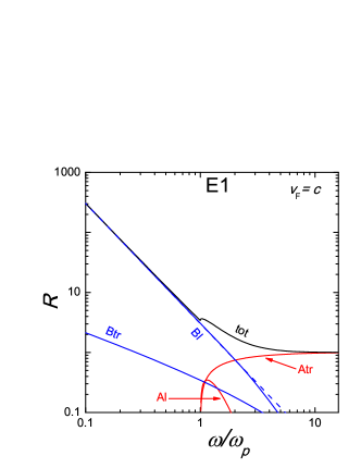
Figure 1: (Color online). Different partial contributions to the total plasma enhancement factor $R$ (curve ‘tot’) as a function of $\omega/\omega_{p}$ for E1 transitions at $v_{F}=c$. Other solid curves show $R_{\mathrm{Btr}}$, $R_{\mathrm{Bl}}$, $R_{\mathrm{Al}}$, and $R_{\mathrm{Atr}}$. The dashed curve is the low-$\omega$ asymptote $R_{\mathrm{Bl}}=3.03\,\omega_{p}^{2}/\omega^{2}$.

In Fig. 1 we plot various plasma factors for an E1 transition rate as a function of $\omega/\omega_{p}$ in the ultrarelativistic strongly degenerate electron plasma ($v_{F}=c$) at $k_{\mathrm{max}}a\ll 1$. The solid line marked ‘tot’ shows the total plasma enhancement factor $R$. Other solid curves are partial contributions $R_{\mathrm{Btr}}$, $R_{\mathrm{Bl}}$, $R_{\mathrm{Al}}$, and $R_{\mathrm{Atr}}$ given by Eqs. (22)–(25). The factors $R_{\mathrm{Al}}$ and $R_{\mathrm{Atr}}$ vanish at $\omega<\omega_{p}$ because no real plasma waves can be emitted under such conditions. At $\omega\gtrsim 3\omega_{p}$ the main contribution to the total transition rate comes from the emission of real transverse plasmons. In the limit of $\omega\gg\omega_{p}$ the plasma effects disappear and $R\approx R_{\mathrm{Atr}}\to 1$. Radiative transitions via virtual longitudinal plasmons always dominate over transitions via virtual transverse plasmon, $R_{\mathrm{Bl}}>R_{\mathrm{Btr}}$. All transitions at $\omega<\omega_{p}$ go via the exchange of virtual plasmons, the transition rate being greatly enhanced in comparison with its in-vacuum value. The dashed line in Fig. 1 shows the low-$\omega$ asymptote $R_{\mathrm{Bl}}=3.03\,\left(\omega_{p}/\omega\right)^{2}$; it is accurate at $\omega<\omega_{p}$, where $R_{\mathrm{Bl}}$ dominates.

Figure 2: Factor $C$ versus $k_{\mathrm{max}}a$ as an illustration of the effect of non-dipole corrections on $R_{\mathrm{Bl}}$ in Eq. (60) for a simplified model of radiative deexcitation of atomic nucleus of radius $a$ (see text). The inset shows $J_{\mathrm{l}}(ka)$ for this model.

All quantities, plotted in Fig. 1, are calculated neglecting non-dipole corrections to the transition current [by setting $J_{\mathrm{l}}(k)=J_{\mathrm{tr}}(k)=1$ that is valid at $k_{\mathrm{max}}a=2p_{F}a/\hbar\ll 1$, see Eqs. (26) and (27)]. The factors $R$ in Fig. 1 are universal, and depend only on $\omega/\omega_{p}$ (in the limit of $v_{F}\to c$). However, the condition $k_{\mathrm{max}}a\ll 1$ can be violated. Such a violation does not significantly affect $R_{\mathrm{Al}}$, $R_{\mathrm{Atr}}$, and $R_{\mathrm{Btr}}$ but can change $R_{\mathrm{Bl}}$ (Sec. IV). The effect of non-dipole corrections on $R_{\mathrm{Bl}}$ is demonstrated in Fig. 2. Now the universality is lost and the result depends on the specific form of the function $J_{\mathrm{l}}(k)$ (determined by the wave functions of the emitter). For illustration, we consider a dipole transition from the lowest excited state with orbital momentum $L=1$ to the ground state ($L=0$) in a spherical potential well of radius $a$ with infinitely high walls (as a very rough model of E1 deexcitation of atomic nucleus). The appropriate function $J_{\mathrm{l}}(ka)$ is shown in the inset. At $\omega\ll\omega_{p}$ we still obtain the asymptote

$$R_{\mathrm{Bl}}=C(k_{\mathrm{max}}a)(\omega_{p}/\omega)^{2},$$ (60)

where $C(k_{\mathrm{max}}a)$ is now determined by $J_{\mathrm{l}}(ka)$ (and does not depend of $\omega_{p}/\omega$). The function $C(k_{\mathrm{max}}a)$ takes into account the non-dipole corrections. It is shown in Fig. 2 for our particular model. The increase of $k_{\mathrm{max}}a$ reduces $C(k_{\mathrm{max}}a)$ with respect to its purely dipole limit $C(0)\approx 3.03$. A reduction by a factor of 2 is achieved at $k_{\mathrm{max}}a\approx 10$.

Thus, non-dipole corrections lower the transition rate, but the rate remains enhanced over its in-vacuum level by a factor of $(\omega_{p}/\omega)^{2}$.This is because the expression for $R_{\mathrm{Bl}}$ (at $\omega<\omega_{p}$) contains the factor $\left(\omega_{p}/\omega\right)^{2}$ which arises from $\Im\,\varepsilon_{\mathrm{l}}(\omega,k)$. The integration over $k$ in Eq. (30) can be carried out using static dielectric function $\varepsilon_{\mathrm{l}}(0,k)$; the function $J_{\mathrm{l}}(k)$ specifies only a numerical prefactor, but does not violate the $\left(\omega_{p}/\omega\right)^{2}$ dependence.

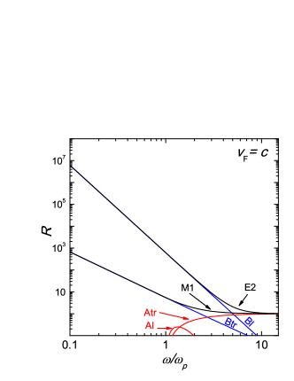
Figure 3: (Color online). Plasma enhancement factors $R_{\mathrm{E2}}$ and $R_{\mathrm{M1}}$ versus $\omega/\omega_{p}$ at $v_{F}=c$, together with the factors $R_{\mathrm{Bl}}^{(2)}$, $R_{\mathrm{Btr}}^{(2)}$, $R_{\mathrm{Al}}^{(2)}$, and $R_{\mathrm{Atr}}^{(2)}$ for separate transition channels.

Now let us consider the E2 and M1 radiative transitions. Their principal features remain the same as for the E1 transitions. In Fig. 3 we plot the plasma enhancement factors $R_{\mathrm{E2}}$ and $R_{\mathrm{M1}}$. One can see that the plasma enhancement of E2 and M1 transitions is stronger than for E1 transitions. However, this is true only if the E1 transition is forbidden. If not, the effect of higher-order transitions (particularly, E2 and M1) is included in the functions $J_{\mathrm{l}}(k)$ and $J_{\mathrm{tr}}(k)$ and has already been discussed above.

Other curves in Fig. 3 show partial contributions to the plasma enhancement factors from different radiative decay channels. The main contribution to E2 transitions comes from $R^{(2)}_{\mathrm{Bl}}$ (as for E1 transitions). Typically higher values of $R^{(2)}_{\mathrm{Bl}}$ [with respect to $R_{\mathrm{Bl}}$ for the E1 case, see Eq. (24)], result from the appearance of an additional $k^{2}$ in the numerator of Eq. (54). This leads to a stronger $\omega_{p}/\omega$ dependence in the asymptotic behavior of $R^{(2)}_{\mathrm{Bl}}$, in comparison with $R_{\mathrm{Bl}}$, $\left(\omega_{p}/\omega\right)^{4}$ instead of $\left(\omega_{p}/\omega\right)^{2}$. Note that the asymptotic expression $R^{(2)}_{\mathrm{Bl}}=607.8\left(\omega_{p}/\omega\right)^{4}$ remains an excellent approximation in the entire range of $\omega$ presented in Fig. 3. Note also, that we have used the first nonvanishing term in the series expansion of the transition current over $ka$. Therefore, our results for E2 and M1 transitions are valid for $2p_{F}\ll\hbar/a$. In the opposite case, just as for the E1 transitions, the results will depend on the exact form of the local transition current $\bm{j}_{fi}(\bm{r})$

We cannot plot the contribution of the additional term, $w_{i\to f}^{\mathrm{L}}$ [see Eq. (57)], to the total transition rate in a similar universal form. If the corresponding moments were equal, then the transition rate in the longitudinal channel in a plasma at $\omega\lesssim\omega_{p}$ would be about twice larger than the E2 transition rate. For $\omega\gg\omega_{p}$ the transition rate $w_{i\to f}^{\mathrm{L}}$ vanishes.

While calculating the $R$-factors, we have used the dielectric function of the degenerate electron gas and have neglected the ion contribution. This approximation is expected to be valid for transition frequencies $\omega$ which are much higher than the ion plasma frequency $\omega_{pi}$ (see Fig. 4). Because $\omega_{pi}\ll\omega_{p}$, the transition frequencies $\omega\lesssim\omega_{pi}$, at which the ion contribution can be important, are much lower than the electron plasma frequency. If necessary, the ion contribution can be studied using similar approach.

The same plasma effects occur in a magnetized plasma but the magnetic field complicates the problem. Because of the anisotropy, introduced into the plasma polarization properties by the magnetic field, the plasma waves (plasmons) become of mixed type (neither longitudinal, nor transverse) and have many branches (for instance, electron cyclotron modes). The properties of the plasmon emission (channels Al and Atr) of an atom in a rarefied magnetoactive cosmic plasma were studied, for instance, in Refs. Kleiman and Oiringel’ (1974); Oiringel’ and Kleiman (1984). The effect of the magnetic field on the processes with virtual plasmons seems to be unexplored.

In our analysis, we have employed zero-temperature approximation but similar effects should be pronounced at finite temperatures. Moreover, thermal plasma fluctuations, available in this case Weisheit (1988), can power inverse transitions and excite the emitter. The efficiency of inverse transitions depends on temperature and plasma parameters.

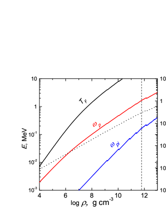
Figure 4: Energy-density diagram (left vertical scale, solid curves) for dense stellar matter. The curves $T_{F}$, $\omega_{p}$ and $\omega_{pi}$ show, respectively, the Fermi energy of degenerate electrons, electron plasma energy $\hbar\omega_{p}$, and ion plasma energy $\hbar\omega_{pi}$ for an accreting neutron star. The short-dashed vertical line positions the neutron drip point. The dotted line (right vertical scale) shows $k_{\mathrm{max}}$ versus $\rho$ to characterize the importance of non-dipole corrections for E1 transitions. See text for details.

The plasma effects are important for studying a number of phenomena in neutron stars and white dwarfs. These effects are outlined below using the energy-density diagram for dense stellar matter (Fig. 4, left vertical scale). The solid lines marked as $T_{F}$, $\omega_{p}$, and $\omega_{pi}$ show the density dependence of the electron degeneracy energy $k_{B}T_{F}$ ($T_{F}$ being the electron degeneracy temperature), as well as the electron and ion plasma energies, $\hbar\omega_{p}$ and $\hbar\omega_{pi}$. For simplicity, we employ the model of accreted neutron star crust (Table A3 from Ref. Haensel and Zdunik (2008)). The curves $T_{F}$ and $\omega_{p}$ are rather insensitive to possible variations of nuclear composition in an accreting neutron star (and quite close to the curves for a neutron star whose crust is composed of the ground-state matter Haensel et al. (2007)). The curve $\omega_{pi}$ is more sensitive to the composition but is relatively unimportant for our analysis. Note that the neutron drip occurs at $\rho\approx 6\times 10^{11}$ g cm^-3 in the accreted crust (and at $\rho\approx 4\times 10^{11}$ g cm^-3 in the ground-state matter). Typical temperatures in neutron stars and white dwarfs are below $10^{9}$ K ($k_{B}T\lesssim 0.1$ MeV). Degenerate electrons become relativistic at $\rho\gtrsim 10^{6}$ g cm^-3.

Plasma effects can affect beta captures in dense stellar matter, for instance, in the crust of an accreting neutron star in a binary system with a low-mass companion. Such systems manifest themselves as X-ray transients which demonstrate periods of active accretion and quiescence Chen et al. (1997). Observations show that neutron stars in X-ray transients remain warm during quiescent periods that is often explained Brown et al. (1998) by deep crustal heating associated with nuclear transformations Haensel and Zdunik (1990); Gupta et al. (2007); Haensel and Zdunik (2008), particularly, beta captures, in the accreted matter. When the accreted matter is gradually compressed by newly accreted material, the density in local matter elements goes up increasing the Fermi energy of degenerate electrons. This triggers beta captures with the appearance of daughter nuclei in ground or excited states. If the daughter nuclei are born in the excited states, they can de-excite through radiative transitions Gupta et al. (2007); the associated energy release can contribute to the deep crustal heating. The nuclear composition of the accreted matter can be very different and contain a wide spectrum of nuclides Gupta et al. (2007). This means numerous beta captures involving various nuclei at the densities up to $10^{11}-10^{12}$ g cm^-3 (Fig. 4). In this case the electron gas is strongly degenerate and ultrarelativistic, the electron plasma energy $\hbar\omega_{p}$ can reach a few MeV and become larger than transition energies $\hbar\omega$ in some nuclei. What will happen with these nuclei? A naive answer would be that they would not decay to lower states because they cannot emit any electromagnetic quanta at $\omega<\omega_{p}$. Our results show quite the opposite. The plasma environment enhances the decays through the processes B involving virtual (mostly longitudinal) plasmons. The dotted line in Fig. 4 plots (right vertical scale) the values of $k_{\mathrm{max}}$. As follows from the above discussion (see Fig. 2), at $k_{\mathrm{max}}a\gtrsim 10$ our plasma enhancement factor for E1 transitions starts to deviate from the universal enhancement (33). The dotted line indicates that, for typical radii $a$ of atomic nuclei, we have $k_{\mathrm{max}}a\lesssim 10$ at any $\rho$ in Fig. 4, so that the enhancement remains universal. Let us stress, however, that we use a very crude model of E1 transition in Fig. 2. We would advise to check the condition for the breaking of universality (33) in specific situations.

Another example is provided by the reactions involving neutrons (n) in accreting neutron stars Gupta et al. (2008). Specifically, we mean the reactions (n,$\gamma$) and ($\gamma$,n) (neutron absorption by a nucleus with the emission of electromagnetic quantum, and an inverse process). These reactions can occur at densities $10^{11}-10^{12}$ g cm^-3 near the neutron drip density in the neutron star crust (Fig. 4). They can accompany deep nuclear burning of accreted matter and affect energy release and nuclear transformations in deep crustal heating process as well as X-ray superbursts (highly energetic X-ray bursts demonstrated by some accreting neutron stars). Again, many nuclei can be involved, and typical energies $\hbar\omega$ of electromagnetic transitions can be lower than $\hbar\omega_{p}$. Our results cannot be used directly to study the neutron reactions, but they can be modified for that purpose. They demonstrate that the plasma effects cannot suppress Gupta et al. (2008) the neutron capture reactions (n,$\gamma$) at $\omega_{p}>\omega$. Moreover, we can expect that even at $\omega\ll\omega_{p}$, but at not very low temperatures, there will be a substantial level of fluctuating plasma microfields (associated with virtual plasmons) to power the inverse reaction ($\gamma$,n).

Finally, the present results can be useful for calculating the radiative thermal conductivity in a degenerate electron gas. This is an important problem for outer cores of white dwarfs and outer envelopes of neutron stars, where the radiative conduction becomes comparable to the electron one (the latter dominates in the deeper, strongly degenerate layers of these objects; see, e.g., Ref. Potekhin et al. (1997)). With increasing density into the degenerate matter, the electron plasma frequency becomes comparable to typical radiative transition frequencies ($\omega\sim k_{B}T/\hbar$) and then exceeds them. Radiative conduction is provided by real electromagnetic waves (not virtual excitations), which leads to the plasma cutoff of the radiative thermal conductivity at low temperatures ($k_{B}T\ll\hbar\omega_{p}$, Fig. 4). This cutoff has been mentioned in the astrophysical literature (e.g., Buchler and Yueh (1976)). A general physical theory of radiative transfer in dispersive media was constructed long ago Harris (1965). Several attempts have been made (e.g., Aharony and Opher (1979); Yu. K. Kurilenkov and Van Horn (1994)) to calculate the radiative thermal conductivity in dense stellar matter with account for the plasma effects. However, these calculations have neglected the contribution of longitudinal plasmons which is expected to be important at $k_{B}T\lesssim\hbar\omega_{p}$, especially in the non-relativistic mildly degenerate electron gas ($T\sim T_{F}$) where the radiative thermal conductivity can be comparable with the electron one.

VII Conclusions

We have analyzed the radiative transition rate of an emitter (an atom or atomic nucleus) immersed in a dense degenerate plasma. Such a transition goes, generally, through four channels which involve real and virtual longitudinal and transverse plasmons (Refs. Klimontovich (1983); Oiringel’ and Kleiman (1984); Table 1). The emission of real plasmons is allowed only at radiative transition frequencies $\omega$ higher than the electron plasma frequency $\omega_{p}$. The processes with virtual plasmons operate at any $\omega$.

Our main conclusions are:

1. The cumulative effect of the plasma is to enhance the radiative decay rate over the standard radiative decay rate through the emission of photons in vacuum. In the limit of $\omega\gg\omega_{p}$ the plasma enhancement effect disappears.

2. The enhancement becomes especially strong at $\omega\ll\omega_{p}$ (where real plasmons cannot exist at all), being mainly provided by processes with virtual longitudinal plasmons.

3. The plasma enhancement takes place for electric dipole transitions, and for higher-order transitions (such as electric quadrupole and magnetic dipole one); it is more pronounced for higher-order transitions.

4. In a strongly degenerate ultrarelativistic electron plasma the plasma enhancement depends mainly on the parameter $\omega/\omega_{p}$. This dependence is calculated and approximated by analytic expressions for E1, E2 and M2 transitions.

The plasma enhancement effects can strongly modify radiative thermal conduction in dense stellar matter, kinetics of atomic nuclei in excited states, emission and absorption of neutrons. Such effects can be important in degenerate cores of white dwarfs and envelopes of neutron stars but are almost unexplored.