Non-Steady State Accretion Disks in X-Ray Novae: Outburst Models for Nova Monocerotis 1975 and Nova Muscae 1991

Abstract

We fit outbursts of two X-ray novae (Nova Monocerotis 1975 = A 0620–00 and Nova Muscae 1991 = GS 1124–683) using a time-dependent accretion disk model. The model is based on a new solution for a diffusion-type equation for the non-steady-state accretion and describes the evolution of a viscous $\alpha$–disk in a binary system after the peak of an outburst, when matter in the disk is totally ionized. The accretion rate in the disk decreases according to a power law. We derive formulas for the accretion rate and effective temperature of the disk. The model has three free input parameters: the mass of the central object $M$, the turbulence parameter $\alpha$, and the normalization parameter $\delta t$. Results of the modeling are compared with the observed X-ray and optical B and V light curves. The resulting estimates for the turbulence parameter $\alpha$ are similar: 0.2–0.4 for A 0620–00 and 0.45–0.65 for GS 1124–683, suggesting a similar nature for the viscosity in the accretion disks around the compact objects in these sources. We also derive the distances to these systems as functions of the masses of their compact objects.
DOI: 10.1134/1.1479424
 
 
 

1 Introduction

Accretion provides an efficient mechanism for energy release in stellar systems, making many astrophysical objects observable. If the matter captured by the gravitation of the central body possesses nonzero angular momentum relative to this body, accretion occurs in a disk. This is true, for example, in binaries, where the angular momentum is associated with the orbital rotation of the components. In the course of accretion onto a compact object whose radius is comparable to the gravitational radius, a substantial fraction of the total energy of the accreted matter $mc^{2}$ is released.

Outbursts reflect one of the most fundamental properties of accretion: its non-steady-state character. Currently, a number of different models are proposed to explain non-steady-state processes in accretion disks and to describe the observed source variability. One problem is to find an adequate description for the viscosity in the accretion disk: viscosity is essential for the accretion, and the viscosity characteristics specify the features of time-dependent disk behavior.

In Lipunova & Shakura (2000), a new solution for the basic equation of time-dependent disk accretion is found and applied to a model of an accretion $\alpha$–disk around a compact star in a close binary. An important property of the disk in a binary system is that its outer radius is limited. Angular momentum is carried away from the outer boundary of the disk due to tidal forces, so that the rotation of outer parts of the disk is synchronized with the rotation of the secondary. It is assumed that the size of the accretion disk specified by the tidal interactions is constant over the time interval considered. Another assumption is that the rate of mass transfer from the secondary to the disk is small compared to the accretion rate within the disk.

The last condition is satisfied, for example, in an X-ray nova outburst. The accretion rate in the disk during the outburst reaches tenths of the Eddington rate $10^{-9}~{}(\vartheta\,M/M_{\odot})~{}M_{\odot}/$yr or more, where $\theta$ is the accretion efficiency and $M$ is the mass of the central object), while the observed rate of mass transfer from the companion in quiescent periods is $10^{-11}$–$10^{-12}~{}M_{\odot}/$yr (Tanaka & Shibazaki, 1996; Cherepashchuk, 2000). X-ray novae are low-mass binaries containing a black hole or a neutron star (see, for example, Cherepashchuk (2000)). The other component, a low-mass dwarf, fills its Roche lobe, so matter continuously flows into the disk (Cherepashchuk, 2000).

Currently, more than 30 X-ray novae are known (Cherepashchuk, 2000). Most of them have light curves with similar exponentially decreasing profiles (Chen et al., 1997). During the burst rise, the intensity increases by a factor of $10^{2}$–$10^{6}$ over several days, whereas the exponential decrease of the light curve lasts for several months, with a characteristic time of about 30–40 days.

Two mechanisms for X-ray nova outbursts are developed: disk instability and unstable mass transfer from the secondary. A final choice between them has not been made, and each model faces some problems (see, for example, Cherepashchuk (2000)). In disk-instability models, during the outburst, the central object accretes matter accumulated by the disk over decades of the quiescent state. This idea is supported by the fact that the mass-transfer rate in quiescent periods is comparable to an accretion rate corresponding to the outburst energy divided by the time between outbursts (Tanaka & Shibazaki, 1996).

In any case, an important point here is that we assume the presence of a standard disk at the time of maximum brightness of the source, as confirmed by spectral observations (Tanaka & Shibazaki, 1996). By ”standard disk” we mean a multi-color $\alpha$–disk whose inner radius coincides with the last stable orbit around the black hole, with the velocity of radial motion of gas being small compared to other characteristic velocities in the disk. Then, the solution of Lipunova & Shakura (2000) can be applied to the decay of an X-ray nova outburst. The light curve calculated using the solution describes observations when the contribution of the accretion disk dominates in the soft X-ray radiation of the system. This phase is characterized by a definite spectral state and can be distinguished in the evolution of an X-ray nova.

Modeling the light curves of an X-ray nova in several X-ray and optical bands enables one to derive the basic parameter of the disk, the turbulence parameter $\alpha$ (this is a new, independent method for determining $\alpha$ in astrophysical disks), as well as the relationship between the distance and mass of the compact component.

Here, we apply our model to Nova Monocerotis A 0620–00, which is the brightest nova in X-rays observed to the present time, and Nova Muscae GS 1124–683.

Currently, the most likely mechanism for turbulence and angular-momentum transfer in accretion disks is thought to be Velikhov–Chandrasekhar magnetic–rotational instability (Velikhov, 1959; Chandrasekhar, 1961), which is investigated in application to accretion disks by Balbus & Hawley (1991). Calculations suggest that this type of instability corresponds to $\alpha\sim 10^{-2}$.

The parameter $\alpha$, which was introduced by Shakura (1972), describes large-scale turbulent motions. The large-scale development of MHD turbulence has been simulated, for example, by Armitage (1998) and Hawley (2000), and it was estimated that $\alpha\sim 10^{-1}$.

On the other hand, the following estimates for $\alpha$ were derived by comparing theory and observations: for dwarf novae $\sim 0.1$ during an outburst and $\sim 0.02$ in a quiescent state in a model with a limit-cycle instability (see, for example, Cannizzo et al. (1988)); $\sim 10^{-2}$ for disks in galactic nuclei (Siemiginowska & Czerny, 1989); $\sim 1$ for Sgr A^∗ in an advection-dominated model (Narayan et al., 1995); and $\sim 0.1-0.3$ in the inner, hot advective part of the disk for the X-ray novae GS 1124–683, A 0620–00, and V404 Cyg, basing on spectra in the low state (Narayan et al., 1996).

2 MODEL FOR ACCRETION DISKS IN X-RAY NOVAE

The evolution of a viscous accretion disk is described by the diffusion-type nonlinear differential equation (Filipov, 1984):

$$\frac{\partial F}{\partial t}=D\,\frac{F^{m}}{h^{n}}\,\frac{\partial^{2}F}{\partial h^{2}}\,,$$ (1)

where $F=W_{r\varphi}\,r^{2}$ is the total moment of the viscous forces acting between adjacent rings of the disk divided by $2\pi$, $W_{r\varphi}$ is the component $w_{r\varphi}$ of the viscous stress tensor integrated over the thickness of the disk, $h=\sqrt{GMr}$ is the specific angular momentum, and $M$ is the mass of the central object. The dimensionless constants $m$ and $n$ depend on the type of opacity in the disk. If the opacity is determined largely by absorption (free–free and bound–free transitions), then $m=3/10$ and $n=4/5$. The “diffusion coefficient” $D$ specified by the vertical structure of the disk relates the surface density $\Sigma$, $F$ , and $h$ (Filipov, 1984; Lyubarskij & Shakura, 1987):

$$\Sigma=\frac{(GM)^{2}\,F^{1-m}}{2\,(1-m)\,D\,h^{3-n}}\,.$$ (2)

Relation (2) is derived from an analysis of the vertical structure of the disk.

A class of solutions for Eq. (1) is derived in Lyubarskij & Shakura (1987) during studies of the evolution of a torus of matter around the gravitating center under the action of viscous forces, which are parameterized by the turbulent viscosity parameter $\alpha$ introduced in Shakura (1972). In particular, a solution was obtained for the stage when the torus has evolved to an accretion-disk configuration, from which matter flows onto the central object. When the accretion rate through the inner edge decreases, the outer radius of the disk simultaneously increases—the matter carries angular momentum away from the center. In this model, the accretion rate decreases with time as a power law. The power-law index depends on the type of opacity in the disk.

An important property of a disk in a binary system is the cutoff of the disk at the outer radius, in the region where the angular momentum is carried away due to the orbital motion (see, for example, Ichikawa & Osaki (1994)). Taking into account the corresponding boundary conditions, we obtained a new solution for Eq. (1) in a general form for a disk with uniform opacity (Lipunova & Shakura, 2000). We described the vertical structure using calculations of Ketsaris & Shakura (1998) in the framework of the generally accepted $\alpha$-disk model (Shakura & Sunyaev, 1973). Following Lyubarskij & Shakura (1987), we considered two opacity regimes: with the dominant contribution to the opacity made by the Thomson scattering of photons on free electrons, and by the free–free and bound–free transitions in the plasma. As a result, we obtained explicit expressions describing the time variations of the physical parameters of the accretion disk. The solution describes the evolution of the accretion disk in a binary during the decay of the outburst, while the matter in the disk remains completely ionized. The accretion rate decreases with time according to a power law; however, in this case, the power-law index is larger than that for the solution of Lyubarskij & Shakura (1987): $-5/2$ compared to $-19/16$ when Thomson scattering dominates and $-10/3$ compared to $-5/4$ when absorption dominates. The solutions in the two opacity regimes join smoothly, providing a basis for applying a combined solution to describe the evolution of a disk with a realistic opacity. Our study of disks in stellar binary systems indicates that the second opacity regime is realized during times investigated.

The law for the variation of the accretion rate can be easily derived from the condition of mass conservation in the disk. Let a Keplerian $\alpha$–disk in a binary have fixed inner and outer radii $r_{\mathrm{in}}$ and $r_{\mathrm{out}}$. The mass of the disk is $M_{\mathrm{d}}=\int\limits_{r_{\mathrm{in}}}^{r_{\mathrm{out}}}2\,\pi\,r\,\Sigma\,\mathrm{d}r$. If this mass varies only due to accretion through the inner disk boundary (i.e., the accretion rate onto the outer boundary is substantially lower), then $\mathrm{d}M_{\mathrm{d}}/\mathrm{d}t=\dot{M}_{\mathrm{in}}(t)$. Let the disk parameters $F$ and $\Sigma$ be represented as the products $F(t)\,f(\xi)$ and $\Sigma(t)\,\sigma(\xi)$, where $f(\xi)$ and $\sigma(\xi)$ are dimensionless functions of the radial coordinate $\xi=h/h_{\mathrm{o}}$. The value of $h_{\mathrm{o}}$ is fixed and equal to the angular momentum at the outer disk boundary. Let us express the surface density $\Sigma$ in the integrand in terms of $F$ using Eq. (2). It follows from the equation for the angular momentum transfer that $\dot{M}_{\mathrm{in}}(t)=-\,2\,\pi\,F(t)\,f^{\prime}(\xi)/h_{\mathrm{o}}$ (Lipunova & Shakura, 2000); therefore we obtain

$$M_{\mathrm{d}}=-\,\dot{M}_{\mathrm{in}}^{1-m}\,\int\limits_{r_{\mathrm{in}}}^{r_{\mathrm{out}}}\,\left(\frac{h_{\mathrm{o}}\,f(\xi)}{2\,\pi\,y(\xi)}\right)^{1-m}\frac{\pi\,(G\,M)^{2}}{(1-m)\,D\,h^{3-n}}\,r\,\mathrm{d}r\,\\ =\,(\mathrm{d}M_{\mathrm{d}}/\mathrm{d}t)^{1-m}\times const\,,$$ (3)

where dimensionless $y(\xi)=f^{\prime}(\xi)$. We will integrate Eq. (3) over $t$. Using the fact that $m=10/3$ for the Kramers law, we conclude that $M_{\mathrm{d}}\propto(t+\delta\,t)^{-7/3}$ and $\dot{M}_{\mathrm{in}}\propto(t+\delta\,t)^{-10/3}$. Note that, to produce such time dependence, it is sufficient that the “diffusion coefficient” $D$ is constant in time, being a function of the radius.

The bolometric luminosity $L=\theta\dot{M}_{\mathrm{in}}c^{2}$ varies according to the same law as the accretion rate through the inner disk radius. As shown in Lipunova & Shakura (2000), the exponential light curve of an X-ray nova can be then explained if the considered spectral band contains the flux integrated over the exponential falloff in the Wien section of the disk spectrum rather than a fixed fraction of the bolometric luminosity.

In the model considered, the accretion rate depends on the distance from the center. In the central regions, the accretion rate is virtually independent of the radius; but this is not true for the outer disk. The bolometric flux from regions of the disk between rings with radii $0.1\,r_{\mathrm{out}}$ and $r_{\mathrm{out}}$ is about $6$% lower than the values obtained for a stationary standard disk model. The optical flux from the time-dependent disk differs from that from a stationary disk by a smaller amount, depending on a size of the region producing the optical flux. This size is specified by the mass of the central object and the accretion rate in the disk.

To take into account the effects of general relativity in the vicinity of the compact object, we use a modified Newtonian gravitational potential in the form suggested by Paczynsky & Wiita (1980). For a Schwarzschild black hole, this potential is

$$\psi=\frac{G\,M}{r-r_{\mathrm{g}}}~{},$$ (4)

where $r_{\mathrm{g}}=2\,G\,M/c^{2}$. The accretion efficiency $\theta$ for this potential is a factor of $\approx 1.45$ smaller than that for a Newtonian potential.

3 MODELING PROCEDURE

3.1 Derivation of Theoretical Curves

In the model for a time-dependent disk in a binary system (Lipunova & Shakura, 2000), with the opacity in the outer disk defined by the bremsstrahlung absorption, the variation of the accretion rate in the disk as a function of time is given by the formula

$$\dot{M}(h,t)=-2\,\pi\,\frac{1.224\,y(h/h_{\mathrm{o}})}{h_{\mathrm{o}}}\,\left(\frac{h_{\mathrm{o}}^{14/5}}{D\,(t+\delta t)}\right)^{10/3}\,,$$ (5)

where $t$ is the time, $\delta t$, a normalizing shift, $h$, the specific angular momentum, $h_{\mathrm{o}}$, the specific angular momentum of the matter at the outer radius of the disk, $D$, the constant in Eq. (1), and

$$y(\xi)\approx 1.43-1.61\,\xi^{2.5}+0.18\,\xi^{5}\,.$$ (6)

Table 1: Input model parameters. For parameters denoted with ”+” we use observed values.

(1)	(2)	(3)
$M$	Mass of the central object
$M_{\mathrm{o}}$	Mass of the optical component	$+$
$P$	Orbital period of the binary	$+$
$f(M_{\mathrm{o}})$	Mass function of the optical component	$+$
$\alpha$	Turbulence parameter in the disk
$N_{\mathrm{HI}}$	Number of H atoms per cm2 to the source	$+$
$\mu$	Molecular weight of gas in the disk $0.5$
$\delta t$	Inner parameter of the model

Table 1 presents the input parameters for the model. Three parameters are free: the mass of the compact object $M$, the turbulence parameter $\alpha$, and the normalizing parameter $\delta t$. A change of the mass of the optical component $M_{\mathrm{o}}$ affects the disk size, which affects the rate of variation of the accretion rate in the disk. The following values can be obtained from the input parameters:

(1) The system semiaxis $a$, calculated as

$$a=\left(\frac{G\,(M+M_{\mathrm{o}})\,P^{2}}{4\,\pi^{2}}\right)^{1/3}\,,$$ (7)

assuming that the orbits are circular.

(2) The system inclination

$$i=\arcsin{\left(\left[\frac{f(M_{\mathrm{o}})\,(1+q)^{2}}{M\,q^{2}}\right]^{1/3}\right)}\,,$$ (8)

where the mass ratio is $q=M/M_{\mathrm{o}}$.

(3) The radius of the last nonintersecting orbit around the primary, which depends on the mass ratio of the binary components and, in general, does not exceed 0.6 of the Roche lobe size (values are tabulated in Paczynski (1977)); this corresponds to the radius of the outer boundary of the disk $r_{\mathrm{out}}$ (Paczynski, 1977; Ichikawa & Osaki, 1994).

(4) The diffusion coefficient $D$ appeared in Eqs. (1) and (5):

$$D=5.04\times 10^{34}\,\alpha^{4/5}\,(\mu/0.5)^{-3/4}\,(M/M_{\odot})\,B_{\mathrm{f}}~{}~{}\\ [\mbox{g}^{-3/10}\,\mbox{cm}^{5}\,\mbox{s}^{-16/5}]\,,$$ (9)

where $B_{\mathrm{f}}=(\Pi_{1}^{1/2}\,\Pi_{2}\,\Pi_{3}^{8}\,\Pi_{4})^{-1/10}$ is a combination of dimensionless parameters specified by the vertical structure of the disk, calculated and tabulated as functions of the optial depth in Ketsaris & Shakura (1998). Thus, $B_{\mathrm{f}}$ depends on the variable optical depth, which can be obtained from the disk characterstics at the radius. We found that $B_{\mathrm{f}}$ depends stronger on time than on radius, and the time dependence is also not very strong, since $B_{\mathrm{f}}$ is the combination of the parameters raised to powers much smaller than unity. In the modeling, we adopt $B_{\mathrm{f}}\,$ calculated iteratively at the half-radius of the disk and at the middle of the time interval investigated.

To calculate the effective temperature in the disk, we use the formula

$$T^{4}(r)=-\frac{\dot{M}}{4\,\pi\,\sigma}\,\omega(r)\,r\,\frac{\mathrm{d}\omega(r)}{\mathrm{d}r}\,\left(1-\frac{\omega(r_{\mathrm{in}})}{\omega(r)}\,\left(\frac{r_{\mathrm{in}}}{r}\right)^{2}\right)\times\\ \times\sqrt{\frac{r_{\mathrm{out}}}{r}}\,\frac{f(\sqrt{r/r_{\mathrm{out}}})}{f^{\prime}(0)}\,,$$ (10)

where $f(\xi)=1.43\,\xi-0.46\,\xi^{7/2}+0.03\,\xi^{6}$, $\omega(r)$ is the angular velocity in the disk (which is Keplerian away from the compact object), $\sigma$ is the Stefan–Boltzmann constant, and $r_{\mathrm{out}}$ is the radius of the outer boundary of the disk. In Eq. (10), $\dot{M}$ is equal to the value $\dot{M}(0,t)$ defined by Eq. (5). The central regions of the disk (where $r\ll r_{\mathrm{out}}$ and the product of the last two factors in Eq. (10) yields approximately unity) produce the largest contribution to the X-ray emission; here, the accretion rate is nearly constant over radius, and the distribution of the effective temperature essentially coincides with that in a stationary disk. We also take into account non-Newtonian nature of the metric around the compact object in the central regions of the disk. For the Paczynski–Wiita potential (4), one has

$$\omega(r)=\sqrt{\frac{G\,M}{r}}\,\frac{1}{r-r_{\mathrm{g}}}\,.$$ (11)

We assume that the bulk of the optical flux comes from the disk (at distances $r\gg r_{\mathrm{in}}$), while the radiation from the “transition layer” at the outer boundary, where the momentum is carried away, is significantly less.

The spectral flux density detected by an observer can be calculated using the following formula (Bochkarev et al., 1988)

$$F_{\nu}=\frac{L_{\nu}\,\cos{i}}{2\,\pi\,d^{2}}\,\exp{(-\tau_{\nu})}\,~{}[\mbox{erg/cm${}^{2}$\,Hz\,s}]\,,$$ (12)

where $d$ is the distance to the system, not set a-priori in the model, $\tau_{\nu}$ is the optical depth corresponding to the absorption toward the source, and $L_{\nu}$ is the spectral luminosity of two sides of the disk according to the formula

$$L_{\nu}=2\,\pi\,\int\limits_{r_{\mathrm{in}}}^{r_{\mathrm{out}}}{B(\nu,T(r))\,2\,\pi\,r\,\mathrm{d}r}~{}[\mbox{erg}/\mbox{c}\,\mbox{Hz}]\,,$$ (13)

where $B(\nu,T(r))$ is the Planck function.

The model curves $F_{i}$ (erg/cm²s) are calculated by integrating $F_{\nu}$ over frequency. At X-ray energies, $\tau_{\nu}=\sigma(\nu)\,N_{\mathrm{HI}}\,$, and the cross section for absorption by the hydrogen atoms $\sigma(\nu)$ is presented in the form of an analytical spline (Morrison & McCammon, 1983). The number of hydrogen atoms in the line of sight toward the source $N_{\mathrm{HI}}$ can be found in the literature, and can also be calculated using the approximating formula (Zombeck, 1990)

$$N_{\mathrm{HI}}\approx 4.8\times 10^{21}\,E(\mbox{B}-\mbox{V})\,~{}\mbox{\rm{atoms}}/\mbox{\rm{cm}}^{2}\mbox{\rm{mag}}\,,$$ (14)

provided the color excess $E(\mbox{B}-\mbox{V})$ is known and assuming that the main contribution to the absorption is made by the hydrogen atoms of the interstellar medium and not by those directly related to the source.

For the optical spectrum, absorption is taken into account after integrating $F_{\nu}$ over frequency. We use the interstellar absorption $A_{\lambda}=2.5\,\tau/\ln 10$ instead of the optical depth $\tau_{\nu}$; here $\tau$ is some effective value for the optical band denoted by $\lambda$.

We calculate the light curves $F_{i}$ in a chosen time interval $t\in[t_{1},t_{2}]$, and we set $t=0$ at the peak of the outburst. The accretion rate at the inner radius, bolometric luminosity of the disk, and fluxes in specified spectral intervals (the X-ray and the optical B and V bands) are calculated with a step of $\Delta t=1$ day.

3.2 Comparison of the Model and Observed Light Curves

We use the light curves in one X-ray band and in the B and V band.

Spectral observations of X-ray novae can help to determine in which timporal and spectral intervals the flux is dominated by the disk radiation, with much less contributions from other components. In general, it is obviously desirable to use data at the softest X-ray energies (below $\sim 10$ keV), since the typical X-ray spectrum of an X-ray nova after the outburst peak is a combination of the disk spectrum (modeled as emission from a multi-color black-body disk) and a harder power-law component (Tanaka & Shibazaki, 1996). For each source, we must consider the spectral evolution and exclude time intervals when either the contribution from the nondisk components (or power-law components) is substantial or the disk spectrum differs appreciably from that for a multi-color disk model. Nondisk components in the emission can alter the slope of the decaying light curve, and this slope dramatically affects the resulting values of $\alpha$.

We reduce observed stellar magnitudes at optical wavelengths to fluxes in erg/(cm²s) using the formula

$$F_{i}=\Delta\lambda_{i}\,10^{-0.4\,m_{i}-A^{0}_{i}}\,,$$ (15)

where the zero-points $A^{0}_{i}$ and effective bandwidths $\Delta\lambda_{i}$ are presented in Table 2.

Table 2: Zero-points, central wavelengths, and effective widths for the optical bands (Zombeck, 1990). The corrected value is denoted by ^∗; the value from Zombeck (1990) is given in paren theses (see explanation in the text after Eq. (15)).

Band	$A^{0}_{i}$	$\lambda$, Å	$\Delta\lambda_{i}$, Å
U	$8.37$	$3650$	$680$
B	$8.198^{*}$ ($8.18$)	$4400$	$980$
V	$8.44$	$5500$	$890$

We have corrected $A^{0}_{\mathrm{B}}$ values in accordance with Bochkarev et al. (1991), where the disk color indices are calculated using the radial temperature distribution of a standard disk, taking into account the actual transmission functions for the optical filters. The values calculated with our code, using rectangular band-pass for the optical filters, coincide with those from  Bochkarev et al. (1991) to within 0.01^m. To achieve this agreement, it has been necessary to correct the zero-point in the B band.

Let us consider the disk flux $F_{\mathrm{x}}^{\mathrm{obs}}$ observed in some X-ray spectral band at some time $t\in[t_{1},t_{2}]$. We can derive the distance $d$ to the source for the chosen model parameters (see Table 1) by comparing observed flux with theoretical $F_{i}(t)$, taking into account the absorption toward the source and the inclination $i$ calculated with (8). We assume that the disk is coplanar to the binary orbit.

Further, we calculate model light curves $F_{i}$ using the derived $d$. We find the color excess $E(\mbox{B}-\mbox{V})^{\mathrm{model}}$ that is required to obtain agreement with the observed optical flux in the B band. Each optical light curve is then corrected for this $E(\mbox{B}-\mbox{V})^{\mathrm{model}}$ by substructing value $A_{\lambda}/2.5$ from the logarithm of the optical flux. For this, we use the values $R_{\mathrm{B}}=4.2$, $R_{\mathrm{V}}=3.2$, $R_{\mathrm{U}}=5$ (Zombeck, 1990) in the formula relating the color excess and the interstellar absorption:

$$A_{\lambda}=R_{\lambda}\,E(\mathrm{B}-\mathrm{V})\,.$$ (16)

Observations show that certain portions of X-ray light curves of X-ray novae are very close to exponential dependences and, thus, can be described by only two parameters. We approximate the observed light curves with straight lines $\log F_{i}=a_{\mathrm{r}}\,t\,+\,b_{\mathrm{r}}$, whose slopes $a_{\mathrm{r}}$ are to be compared to those of the theoretical curves at some point $t\in[t_{1},t_{2}]$ in the middle of the time interval. For three spectral bands, we fit fluxes at this $t$, taking into account the observed color excess $E(\mbox{B}-\mbox{V})$ and the color of the disk B–V. A set of models is selected to provide a certain agreement between the X-ray and optical fluxes and slopes of the observed and theoretical light curves. The value of $\chi^{2}$ is calculated for the selected models.

A large scatter of the observed disk color B–V, which reaches 0.05 magnitudes (see below), can be caused by both observational errors and possible short-term fluctuations of the disk color (due to precession, the superposition of the optical flux from the secondary, etc.) that we do not examine here. We also do not take into consideration the contribution of radiation from the central X-ray source reradiated from the outer parts of the disk.

For some of the light curves, the overall traces are rather close to exponential, but the exponential law does not agree with the observations by $\chi^{2}$ criterion (at the 0.05 significance level), possibly due to an underestimation of the observational errors, a superposition of fluctuations in emission, and model limitations.

4 MODELING X-RAY NOVA A 0620–00 IN THE 3–6 keV X-RAY AND B AND V OPTICAL BANDS

4.1 Observations

4.1.1 X-ray Light Curves

The nova outburst in Monoceros in 1975 (A 0620–00, V 616 Mon) was observed in X-rays with the orbiting observatories Ariel-5, SAS 3, Salut 4, and Vela 5B (Elvis et al., 1975; Doxsey et al., 1976; Kurt et al., 1976; Kaluzienski et al., 1977; Tsunemi et al., 1989). A 0620–00 was the first X-ray transient identified with an optical burst (Matilsky et al., 1975; Boley et al., 1976).

We take the 3–6 keV data of Kaluzienski et al. (1977), obtained with the Ariel-5 All Sky Monitor. Following Chen et al. (1997), we assume that the peak of the outburst was on Aug 13, 1975, or JD 2442638.3. The corresponding data in Crab flux units are taken in the electronic form from the HEASARC (High Energy Astrophysics Science Archival Research Center) database (Chen et al., 1997).

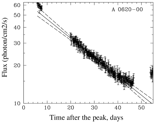
Figure 1: Straight-line approximation of the A 0620–00 X-ray light curve. The regression line for the data in the interval $t\in[20,40]$ days (solid line) and selection boundaries for the theoretical curves (two dashed lines) are plotted. The observational data are from Kaluzienski et al. (1977).

We fit the X-ray light curve in units of photons/cm²s. Figure 1 illustrates selection of models according to the slope of the 3–6 keV X-ray light curve at $t=30$ day. The regression line constructed using observations in the interval $t\in[20,40]$ day has $a_{\mathrm{r}}=-0.01502\pm 0.0002$ and $b_{\mathrm{r}}=1.816\pm 0.007$. The data at $t\approx 10$ days cannot be ascribed with confidence to the exponential section of the light curve caused by the disk radiation. The dashed curves indicate the boundaries within which we select the models. Within these boundaries, the slopes of the lines vary in the range $(0.9-1.1)\,a_{\mathrm{r}}$. Value of $\chi^{2}$, calculated for the observational data and the lines with such slopes, divided by the number of degrees of freedom, does not exceed 1.3.

4.1.2 X-ray Spectrum at the Time of the Outburst

As has often been noted, X-ray novae in general and A 0620–00 in particular (see, for example, Kuulkers (1998)) display softening of the spectrum during the initial decay in the light curve. For A 0620–00, this was pointed out, for example, by Carpenter et al. (1976) for 3.0–7.6 keV observations and Citterio et al. (1976), for 3–9 keV.

Spectral data with high resolution (10 eV at 2 keV and 285 eV at 6.7 keV) obtained with the Columbia spectrometer OSO 8 on board the Ariel-5 spacecraft in October 1975 were analyzed in Long & Kestenbaum (1978). The X-ray continuum of A 0620–00 on September 17–18, 1975 (the 34–35th day after the peak) was best fit by a blackbody model with $kT\sim 0.5$ keV.

Note that, at the energies of interest to us ($>1$ keV), the spectrum of a multi-color, blackbody disk can be approximated by a Wien spectrum:

$$I_{E}=\frac{2}{c^{2}\,h^{3}}\,{E^{3}}\,{\exp{(-E/kT_{\mathrm{max}})}}\ ,$$ (17)

where $T_{\mathrm{max}}$ is the maximum temperature in the disk, which occurs at the radius $\approx 1.58\,r_{\mathrm{in}}$ in the case of the Paczynski–Wiita gravitational potential (4). In a Newtonian potential approximation, the radius for the maximum temperature is approximately $1.36\,r_{\mathrm{in}}$.

Number of Hydrogen Atoms/cm² toward A 0620–00 and the Color Excess

The number of hydrogen atoms was estimated from the falloff in the soft X-ray spectrum due to the absorption of X-rays with energies $<1$ keV (Carpenter et al., 1976; Doxsey et al., 1976; Kurt et al., 1976): $3\times 10^{21}-10^{22}$ atoms/cm².

In Wu et al. (1983), the estimate $E(\mbox{B}-\mbox{V})=0.35$ was derived using UV observations obtained with the ANS satellite. Twenty-five stars around A 0620–00 were studied, and a specific absorption curve for the region was derived. Using (14), one finds $N_{\mathrm{HI}}\sim 1.7\times 10^{21}$ atoms/cm². The total number of hydrogen atoms in the Galaxy in the line of sight toward A 0620–00 is $\sim 4\times 10^{21}$ atoms/cm² (Weaver & Williams, 1974).

Obviously, we cannot exclude the possibility of substantial and variable absorption of the X-ray radiation in the source itself. However, the character and origin of this variability are unknown. We model the observations for Nova Monocerotis for a set of $N_{\mathrm{HI}}$ values in the range $10^{21}$–$10^{22}$ atoms/cm². For the color excess, we adopt value $E(\mbox{B}-\mbox{V})=0.35\pm 0.01$ (Wu et al., 1983).

4.1.3 Optical Light Curves

Optical observations from Liutyi (1976); Shugarov (1976); van den Bergh (1976); Duerbeck & Walter (1976); Robertson et al. (1976); Lloyd et al. (1977) are used. We construct linear regression fits $\log F=a_{\mathrm{r}}\,t\,+\,b_{\mathrm{r}}$ to the B and V optical data in logarithmic flux units for times $t\in[0,47]$ days using the weighted least-squares method. This yields $a_{\mathrm{r}}=-0.0079\pm 0.0002$, $b_{\mathrm{r}}=-9.675\pm 0.005\,$ for the B band and $a_{\mathrm{r}}=-0.0071\pm 0.0002$, $b_{\mathrm{r}}=-9.885\pm 0.006\,$ for the V band (see Section 3.2). The reduced $\chi^{2}$ values for these fits are roughly 12 and 43 for the B and V bands, with 102 and 89 degrees of freedom, respectively. This suggests that the adopted errors for the optical observations might be underestimated (for example, systematic deviations have not been taken into account) and/or that our assumed exponential (quasiexponential) decrease of the optical flux does not yield a complete description of the observed curves, due to various fluctuations and variations of the optical flux superimposed on the overall trace of the light curve. Nevertheless, for modeling we assume that the basic trend of the light curves can be fit by a quasi-exponential decay.

In model fitting, we adopt the color of the disk at $t=30$ days B–V$=0.24\pm 0.03^{m}$, derived from the above observational data.

4.2 Results for A 0620–00

We compare the theoretical and observed curves for $t\in[20,40]$ days after the outburst peak. Table 3 summarizes the parameters attempted. The number of hydrogen atoms along the line of sight toward A 0620–00 does not appreciably affect the results, since the absorption at 3–6 keV is small.

Figure 2: Modeled $\alpha$ and color of the A 0620–00 disk. Results are given for the values from Table 3. The mass of the optical component varies from top to bottom: 0.3, 0.5, and 0.7 $M_{\odot}$. The filled circles satisfy the disk color condition $B-V=0.24\pm 0.03$ mag for $t=30$ days.

Figure 2 presents the results of our modeling for the parameters from Table 3. We can see that $\alpha$ lies in the range 0.225–0.375 (for slightly different masses $M_{\mathrm{o}}$). In Lipunova & Shakura (2001), we adopted $M_{\mathrm{o}}=0.5\,M_{\odot}$ and $E(\mbox{B}-\mbox{V})=0.39$ and used a broader range of slopes than in Fig. 1, so a broader interval for $\alpha$ was obtained for A 0620–00 in that study, from 0.3 to 0.5.

Figure 3: The distance-black hole mass dependence for A 0620–00 for the model parameters from Table 3.

Figure 3 shows the resulting relationship between the distance to A 0620–00 and the mass of the black hole. The distance to A 0620–00 has been estimated to be from 0.5 to 1.2 kpc (for example, in Oke (1977); van den Bergh (1976); see also reviews by Chen et al. (1997); Cherepashchuk (2000)). Figure 3 indicates that for $d\sim 0.9$ kpc (Oke, 1977) the mass of the black hole in A 0620–00 is $\sim 9\,M_{\odot}$. This mass is consistent with previous estimates (see Cherepashchuk (2000) and references therein).

Table 3: Input parameters for A 0620–00 models. The mass of the optical component $M_{\mathrm{o}}=0.5\,M_{\odot}$, its mass function, and the binary period are taken from Chen et al. (1997); Cherepashchuk (2000).

Parameter	Tested values
$M$	$5-25\,M_{\odot}$
$M_{\mathrm{o}}$	$0.3$, $0.5$, $0.7\,M_{\odot}$
$P$	0.322 day
$f(M_{\mathrm{o}})$	$2.7\,M_{\odot}$
$\alpha$	$0.1-1$
$N_{\mathrm{HI}}$	$3\times 10^{21}$–$10^{22}$ atoms/cm2
$\mu$	$0.5$
$\delta t$	$50-250$ days

Figure 4 presents an example of the modeled light curves, with $i=47^{\mathrm{o}}$, $d=0.66$ kpc, the bolometric luminosity $L_{\mathrm{bol}}(t=0)=0.25\,L_{\mathrm{Edd}}\,$, and $T_{\mathrm{max}}(t=35)=0.45$ keV (cf. Section 4.1.2). The reduced $\chi^{2}$ for the X-ray light curve for $t\in[20,40]$ days is 1.17.

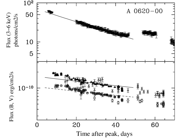
Figure 4: Example of modeling light curves of A 0620–00 in the 3–6 keV, B, and V band. The model parameters are $M=7M_{\odot}$, $M_{o}=0.5M_{\odot}$, $\alpha=0.3$, $\delta t=168$ days, and $N_{\mathrm{HI}}=3\times 10^{21}$ atoms/cm².

We are not able to obtain a satisfactory fit to the slope of the optical light curves. In principle, steeper optical light curves can be obtained by taking into account irradiation of a thick or twisted disk. The outer parts of the disk intercept some of the X-ray flux from the central regions, causing the effective temperature of the outer disk, and accordingly its flux, to increase. The intrinsic and reprocessed flux depend on the accretion rate in different ways: the reradiated optical flux decreases more rapidly, steepening the optical light curves. Esin et al. (2000) have modeled the outburst of A 0620–00 taking into account irradiation of the disk and assuming a relative half-thickness for the disk of 0.12 (which is appreciably higher compared to the standard model). In the standard $\alpha$–disk model, irradiation is insignificant due to the small half-thickness of the disk, which is typically about 0.03 (Lipunova & Shakura, 2000). Probably, a contribution to the optical flux from a disk, which is warped, should be taken into account; a further study of the generation of optical radiation in a time-dependent disk is necessary.

5 MODELING X-RAY NOVA GS 1124–683 IN THE 1.2–37.2 keV X-RAY AND B AND V OPTICAL BANDS

5.1 Observations

5.1.1 X-ray Light Curves

The outburst of Nova Muscae (GS 1124–683, GU Mus) was discovered independently by WATCH/GRANAT and ASM/GINGA (All-Sky X-Ray Monitor) on January 9, 1991 (Lund et al., 1991; Sunyaev, 1991). The associated optical outburst was also detected (Lund et al., 1991). For the modeling, we use 1.2–37.2 keV data obtained with the GINGA Large Area Counters (Ebisawa et al., 1994). The data in erg/(cm²s) are provided by the HEASARC database (Chen et al., 1997, see Footnote 3). Following Chen et al. (1997), we take the peak of the outburst to be on January 15, 1991, or JD 2448272.7862.

The weighted least-squares regression line for data in the interval $t\in[35,61]$ days yields $a_{\mathrm{r}}=-0.0134\pm 0.0001$ and $b_{\mathrm{r}}=-6.511\pm 0.005$. However, the calculated reduced $\chi^{2}$ is very high, since the observational errors are small and the data show an appreciable scatter around the general trend of the model light curve. To select the models, we use interval $(0.98-1.02)\,a_{\mathrm{r}}$ for the the slopes of lines tangent to the theoretical light curves at $t=48$ day.

5.1.2 X-ray Spectrum at the Time of the Outburst

As shown by Ebisawa et al. (1994), after the peak the spectrum of GS 1124–683 softened as the luminosity decreased. In Kitamoto et al. (1992); Miyamoto et al. (1993); Ebisawa et al. (1994); Greiner et al. (1994), the observed X-ray spectrum was approximated by a model with two components: a blackbody, multi-color disk and a harder power-law component. Figure 15 in Ebisawa et al. (1994) indicates that, in the time interval of interest, $T_{\mathrm{in}}$ for the spectral approximation (Ebisawa et al., 1994) is roughly 0.7 keV.

It was suggested by Kitamoto et al. (1992) that 59% of the flux on January 15 (near the outburst peak) was blackbody disk radiation, while the remainder was contributed by a power-law component. During the following 25–30 days, the power-law component decayed more rapidly than the disk component. ROSAT observations on January 25 (the 10th day after the peak) (Greiner et al., 1994) suggested that the 0.3–20 keV flux at that epoch was completely produced by the disk component. Using the approximation for the observed 1.2–37.2 keV X-ray spectrum from Miyamoto et al. (1993) and the derived fluxes of the spectral components, we conclude that the 1.2–37.2 keV flux during $t\in[35,61]$ days after the outburst was determined by the disk radiation and can therefore be used in our modeling, since the contribution from nondisk components is apparently negligible.

Number of Hydrogen Atoms/cm² toward GS 1124–683 and the Color Excess

In Cheng et al. (1992), $E(\mbox{B}-\mbox{V})\sim 0.29$ was estimated from HST observations of the interstellar absorption profile at 2200 Å. Shrader & Gonzalez-Riestra (1993) found $E(\mbox{B}-\mbox{V})=0.3\pm 0.05$ using a similar technique. In della Valle et al. (1991), the same value $E(\mbox{B}-\mbox{V})=0.30\pm 0.10$ was derived from interstellar Na D lines. Using (14), we arrive at $N_{\mathrm{HI}}\approx 1.4\times 10^{21}$ atoms/cm².

Greiner et al. (1994) obtained $N_{\mathrm{HI}}\approx 2.2\times 10^{21}$ atoms/cm² by modeling the combined ROSAT 0.3–4.2 keV and GINGA 1.2–37.2 keV data for January 24–25 using a composite spectrum with a blackbody, multi-color disk and a powerlaw component. For various multi-color disk models, they obtained values from $1.7\times 10^{21}$ to $2.5\times 10^{21}$ atoms/cm².

5.1.3 Optical Light Curves

We use the observational data from King et al. (1996); della Valle et al. (1998) and derive weighted least-squares regression lines for the optical B and V observations in the logarithmic flux units in the time interval $t\in[12,61]$ days. This yields $a_{\mathrm{r}}=-0.0057\pm 0.0006$, $b_{\mathrm{r}}=-10.79\pm 0.03\,$ for the B band, and $a_{\mathrm{r}}=-0.0052\pm 0.0006$, $b_{\mathrm{r}}=-10.98\pm 0.03\,$ for the V band. The corresponding reduced $\chi^{2}$ values are 2.8 and 7.3 for B and V, respectively, with 17 degrees of freedom. This leads us to a conclusion similar to that for A 0620–00 optical light curves (see Section 4.1.3). We again assume that the overall trend of the light curves can be described as quasi-exponential.

In model fitting, we use the observed color of the disk for $t=48$ days: B–V$=0.27\pm 0.07^{m}$.

5.2 Results for GS 1124–683

We compare theoretical and observed curves in the interval $t\in[35,61]$ days after the peak of the outburst.

Table 4: Input parameters for GS 1124–683 models. The mass of the optical component $M_{\mathrm{o}}=0.8\,M_{\odot}$ is adopted from Chen et al. (1997), and the binary period and mass function of the optical component $3.01\pm 0.15M_{\odot}$ are from Orosz et al. (1996).

Parameter	Tested values
$M$	$5-25\,M_{\odot}$
$M_{\mathrm{o}}$	$0.8,0.9\,M_{\odot}$
$P$	0.433 days
$f(M_{\mathrm{o}})$	$3\,M_{\odot}$
$\alpha$	$0.1-1$
$N_{\mathrm{HI}}$	$(1.4-2.5)\times 10^{21}$ atoms/cm2
$\mu$	$0.5$
$\delta t$	$50-250$ days

Figure 5: Modeled $\alpha$ and color of the disk of GS 1124–683 for the parameters in Table 4. The mass of the optical component and the number of hydrogen atoms along the line of sight toward GS 1124–683 vary from top to bottom: $M_{o}=0.8M_{\odot}$, $N_{\mathrm{HI}}=1.4\times 10^{21}$ atoms/cm² (two upper graphs), $M_{o}=0.9M_{\odot}$ , $N_{\mathrm{HI}}=1.4\times 10^{21}\mathrm{atoms/cm}^{2}$ (two middle graphs), and $M_{o}=0.8M_{\odot}$, $N_{\mathrm{HI}}=2.5\times 10^{21}\mathrm{atoms/cm}^{2}$ (two lower graphs). The filled circles satisfy the disk color condition $B-V=0.27\pm 0.07$ mag for $t=48$ days.

Figure 5 presents the results of our modeling for the parameters from Table 4. Comparing the lower and upper left graphs, we can see a slight dependence of the results on the number of hydrogen atoms toward GS 1124–683. The resulting $\alpha$ values for the GS 1124–683 disk lie in the range 0.475–0.625 (for small variations in $M_{\mathrm{o}}$ and $N_{\mathrm{HI}}$).

Figure 6: The distance-black hole mass relation for GS 1124–683, modeled for the parameters from Table 4.

Figure 6 displays the dependence of the distance to GS 1124–683 on the black hole mass. Estimates of the distance to GS 1124–683 in the literature range from 1 to 8 kpc. For 3 kpc (Cherepashchuk, 2000), the implied mass of the black hole in GS 1124–683 is $\sim 8\,M_{\odot}$ (Fig. 6). The values for the black-hole mass obtained by us are consistent with the observations (see Cherepashchuk (2000) and references therein).

Figure 7 presents model light curves for a particular choice of parameters. In the corresponding model $i=68^{\mathrm{o}}$, $d=2.6$ kpc, the bolometric luminosity $L_{\mathrm{bol}}(t=0)=0.47\,L_{\mathrm{Edd}}\,$, and $T_{\mathrm{max}}(t=48)=0.44$ keV. The model satisfactorily reproduces both the X-ray and optical-light curves of GS 1124–683.

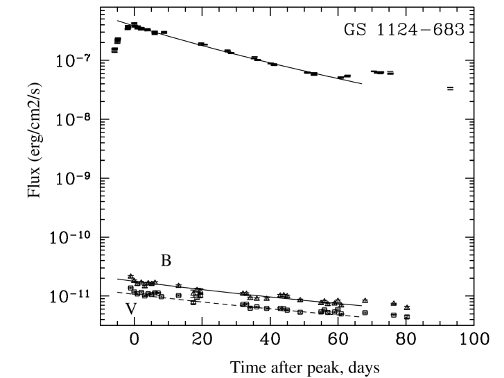
Figure 7: Example of modeling light curves of GS 1124–683 in the 1.2–37.2 keV, B, and V band. The model parameters are $M=7M_{\odot}$, $M_{o}=0.8M_{\odot}$, $\alpha=0.55$, $\delta t=103$ days, and $N_{\mathrm{HI}}=1.4\times 10^{21}\mathrm{atoms/cm}^{2}$.

6 CONCLUSION

We have modeled outbursts of two X-ray novae, A 0620–00 and GS 1124–683, using the model of a time-dependent $\alpha$–disk in a binary system developed in Lipunova & Shakura (2000).

The turbulence parameter $\alpha$ is estimated as 0.2–0.4 for A 0620–00 and 0.45–0.65 for GS 1124–683. The estimates of $\alpha$ are close to each other, indicating the common nature for viscosity in the accretion disks around compact objects, at least in these two sources. The value of $\alpha$ ($\lesssim 1$) points out that the gas in the disks is appreciably turbulent. We have also obtained relations between the distances to the systems and the masses of the compact objects.

Thus, it is possible for the first time to model exponentially decaying light curves of X-ray novae using a model with a thin accretion disk with constant $\alpha$ and estimate value of $\alpha$.

Note that the optical B and V fluxes from GS 1124–683 can be explained as the disk radiation generated locally due to viscous heating. It is likely that in the case of A 0620–00, we must also take into account the contribution of reradiation by a warped disk. We will consider this problem in a subsequent paper.

7 ACKNOWLEDGEMENTS

The authors are grateful to V.F. Suleimanov for useful discussions. This work is supported by the Russian Foundation for Basic Research (project nos. 01–02–06268, 00–02–17164), the “Universities of Russia” program (project no. 5559), and the State Science and Technology Project “Astronomy” (project 1.4.4.1). GVL is also grateful for financial support from the “Young Scientists of Russia” program (www.rsci.ru, 2001). Primary translation is done by K. Maslennikov.

References

- Armitage (1998) Armitage P. J., 1998, ApJ, 501, L189
- Balbus & Hawley (1991) Balbus S. A., Hawley J. F., 1991, ApJ, 376, 214
- Bochkarev et al. (1991) Bochkarev N. G., Karitskaya E. A., Shakura N. I., Zhekov S. A., 1991, Astronomical and Astrophysical Transactions, 1, 41
- Bochkarev et al. (1988) Bochkarev N. G., Syunyaev R. A., Khruzina T. S., Cherepashchuk A. M., Shakura N. I., 1988, Soviet Astronomy, 32, 405
- Boley et al. (1976) Boley F., Wolfson R., Bradt H., Doxsey R., Jernigan G., Hiltner W. A., 1976, ApJ, 203, L13+
- Cannizzo et al. (1988) Cannizzo J. K., Shafter A. W., Wheeler J. C., 1988, ApJ, 333, 227
- Carpenter et al. (1976) Carpenter G. F., Eyles C. J., Skinner G. K., Willmore A. P., Wilson A. M., 1976, MNRAS, 176, 397
- Chandrasekhar (1961) Chandrasekhar S., 1961, Hydrodynamic and hydromagnetic stability. International Series of Monographs on Physics, Oxford: Clarendon, 1961
- Chen et al. (1997) Chen W., Shrader C. R., Livio M., 1997, ApJ, 491, 312
- Cheng et al. (1992) Cheng F. H., Horne K., Panagia N., Shrader C. R., Gilmozzi R., Paresce F., Lund N., 1992, ApJ, 397, 664
- Cherepashchuk (2000) Cherepashchuk A. M., 2000, Space Science Reviews, 93, 473
- Citterio et al. (1976) Citterio O., Conti G., di Benedetto P., Tanzi E. G., Perola G. C., White N. E., Charles P. A., Sanford P. W., 1976, MNRAS, 175, 35P
- della Valle et al. (1991) della Valle M., Jarvis B. J., West R. M., 1991, Nature, 353, 50
- della Valle et al. (1998) della Valle M., Masetti N., Bianchini A., 1998, A&A, 329, 606
- Doxsey et al. (1976) Doxsey R., Jernigan G., Hearn D., Bradt H., Buff J., Clark G. W., Delvaille J., Epstein A., Joss P. C., Matilsky T., Mayer W., McClintock J., Rappaport S., Richardson J., Schnopper H., 1976, ApJ, 203, L9
- Duerbeck & Walter (1976) Duerbeck H. W., Walter K., 1976, A&A, 48, 141
- Ebisawa et al. (1994) Ebisawa K., Ogawa M., Aoki T., Dotani T., Takizawa M., Tanaka Y., Yoshida K., Miyamoto S., Iga S., Hayashida K., Kitamoto S., Terada K., 1994, PASJ, 46, 375
- Elvis et al. (1975) Elvis M., Page C. G., Pounds K. A., Ricketts M. J., Turner M. J. L., 1975, Nature, 257, 656
- Esin et al. (2000) Esin A. A., Kuulkers E., McClintock J. E., Narayan R., 2000, ApJ, 532, 1069
- Filipov (1984) Filipov L. G., 1984, Advances in Space Research, 3, 305
- Greiner et al. (1994) Greiner J., Hasinger G., Molendi S., Ebisawa K., 1994, A&A, 285, 509
- Hawley (2000) Hawley J. F., 2000, ApJ, 528, 462
- Ichikawa & Osaki (1994) Ichikawa S., Osaki Y., 1994, PASJ, 46, 621
- Kaluzienski et al. (1977) Kaluzienski L. J., Holt S. S., Boldt E. A., Serlemitsos P. J., 1977, ApJ, 212, 203
- Ketsaris & Shakura (1998) Ketsaris N. A., Shakura N. I., 1998, Astronomical and Astrophysical Transactions, 15, 193
- King et al. (1996) King N. L., Harrison T. E., McNamara B. J., 1996, AJ, 111, 1675
- Kitamoto et al. (1992) Kitamoto S., Tsunemi H., Miyamoto S., Hayashida K., 1992, ApJ, 394, 609
- Kurt et al. (1976) Kurt V. G., Moskalenko E. I., Titarchuk L. G., Sheffer E. K., 1976, Soviet Astronomy Letters, 2, 42
- Kuulkers (1998) Kuulkers E., 1998, New Astronomy Review, 42, 1
- Lipunova & Shakura (2000) Lipunova G. V., Shakura N. I., 2000, A&A, 356, 363
- Lipunova & Shakura (2001) Lipunova G. V., Shakura N. I., 2001, Astrophysics and Space Science Supplement, 276, 231
- Liutyi (1976) Liutyi V. M., 1976, Soviet Astronomy Letters, 2, 43
- Lloyd et al. (1977) Lloyd C., Noble R., Penston M. V., 1977, MNRAS, 179, 675
- Long & Kestenbaum (1978) Long K. S., Kestenbaum H. L., 1978, ApJ, 226, 271
- Lund et al. (1991) Lund N., Brandt S., Makino F., McNaught R. H., Jones A., West R. M., 1991, IAU Circ., 5161, 1
- Lyubarskij & Shakura (1987) Lyubarskij Y. E., Shakura N. I., 1987, Soviet Astronomy Letters, 13, 386
- Matilsky et al. (1975) Matilsky T., Boley F., Wolfson R., Gull T., York D., 1975, IAU Circ., 2819, 1
- Miyamoto et al. (1993) Miyamoto S., Iga S., Kitamoto S., Kamado Y., 1993, ApJ, 403, L39
- Morrison & McCammon (1983) Morrison R., McCammon D., 1983, ApJ, 270, 119
- Narayan et al. (1996) Narayan R., McClintock J. E., Yi I., 1996, ApJ, 457, 821
- Narayan et al. (1995) Narayan R., Yi I., Mahadevan R., 1995, Nature, 374, 623
- Oke (1977) Oke J. B., 1977, ApJ, 217, 181
- Orosz et al. (1996) Orosz J. A., Bailyn C. D., McClintock J. E., Remillard R. A., 1996, ApJ, 468, 380
- Paczynski (1977) Paczynski B., 1977, ApJ, 216, 822
- Paczynsky & Wiita (1980) Paczynsky B., Wiita P. J., 1980, A&A, 88, 23
- Robertson et al. (1976) Robertson B. S. C., Warren P. R., Bywater R. A., 1976, Informational Bulletin on Variable Stars, 1173, 1
- Shakura (1972) Shakura N. I., 1972, AZh, 49, 921
- Shakura & Sunyaev (1973) Shakura N. I., Sunyaev R. A., 1973, A&A, 24, 337
- Shrader & Gonzalez-Riestra (1993) Shrader C. R., Gonzalez-Riestra R., 1993, A&A, 276, 373
- Shugarov (1976) Shugarov S. Y., 1976, Peremennye Zvezdy, 20, 251
- Siemiginowska & Czerny (1989) Siemiginowska A., Czerny B., 1989, MNRAS, 239, 289
- Sunyaev (1991) Sunyaev R., 1991, IAU Circ., 5179, 1
- Tanaka & Shibazaki (1996) Tanaka Y., Shibazaki N., 1996, ARA&A, 34, 607
- Tsunemi et al. (1989) Tsunemi H., Kitamoto S., Okamura S., Roussel-Dupre D., 1989, ApJ, 337, L81
- van den Bergh (1976) van den Bergh S., 1976, AJ, 81, 104
- Velikhov (1959) Velikhov E. P., 1959, Soviet Journal of Experimental and Theoretical Physics, 9, 995
- Weaver & Williams (1974) Weaver H., Williams D. R. W., 1974, A&AS, 17, 1
- Wu et al. (1983) Wu C.-C., Panek R. J., Holm A. V., Schmitz M., Swank J. H., 1983, PASP, 95, 391
- Zombeck (1990) Zombeck M. V., 1990, Handbook of space astronomy and astrophysics. Cambridge: University Press, 1990, 2nd ed.