Effect of third- and fourth-order moments on the modeling of Unresolved Transition Arrays

Abstract

The impact of the third (skewness) and fourth (kurtosis) reduced centered moments on the statistical modeling of E1 lines in complex atomic spectra is investigated through the use of Gram-Charlier, Normal Inverse Gaussian and Generalized Gaussian distributions. It is shown that the modeling of unresolved transition arrays with non-Gaussian distributions may reveal more detailed structures, due essentially to the large value of the kurtosis. In the present work, focus is put essentially on the Generalized Gaussian, the power of the argument in the exponential being constrained by the kurtosis value. The relevance of the new statistical line distribution is checked by comparisons with smoothed detailed line-by-line calculations and through the analysis of $2p\rightarrow 3d$ transitions of recent laser or Z-pinch absorption measurements. The issue of calculating high-order moments is also discussed (Racah algebra, Jucys graphical method, semi-empirical approach …).

1 Introduction

The detailed calculation of all the electric-dipole (E1) line energies and radiative strengths in complex atomic spectra is an overwhelming task. In some circumstances, it can even be useless. Indeed, when the density is sufficiently high so that the physical broadening mechanisms (Stark, …) are important and/or when the number of lines in an energy range becomes large, the lines coalesce into broad structures. Statistical methods are required because, experimentally, some quantities cannot be determined individually, but only as weighted average quantities (this is the case for instance in emission/absorption spectra of highly ionized atoms). Moreover, explicit quantum calculations can be inappropriate, e.g. if the eigenvalues of the hamiltonian are not known with sufficient precision. In addition, global methods can reveal physical properties hidden by a detailed treatment of levels and lines (“one cannot see the wood for the trees”) [1].

A transition array [2] of E1 lines is characterized by a specific distribution of photon energy $E$:

$$I(E)=A(E)~{}\otimes~{}\Psi(E),$$ (1)

where the function $A(E)$ assumes that each line is represented by a Dirac $\delta$-function:

$$A(E)=C_{p}~{}\sum_{a,b}~{}\frac{N_{a}}{g_{a}}~{}\left(E_{ab}\right)^{p}~{}S_{ab}~{}\delta(E-E_{ab})$$ (2)

which, using the appropriate constant factor $C_{p}$, represents either the opacity ($p=1$) or the emissivity of the source ($p=4$). The sum runs over the upper and lower levels of each line belonging to the transition array. The density of ions excited in level $a$ is noted $N_{a}$, and $g_{a}$ is the degeneracy of level $a$. The energy of the line $a\rightarrow b$ is

$$E_{ab}=E_{b}-E_{a}=<b|H|b>-<a|H|a>,$$ (3)

where $H$ is the Hamiltonian of the system and the line strength $S_{ab}$ is equal to $|<a|\mathcal{Z}|b>|^{2}$, where $\mathcal{Z}$ is the $z$ component of the dipole transition operator. The normalized profile $\Psi(E-E_{ab})$ takes into account the broadening of the line in the plasma due to natural width, Doppler effect, ionic Stark effect, electron collisions, etc. In the UTA (Unresolved Transition Arrays) modeling [3], the discrete distribution $A(E)$ can be replaced by a continuous function (usually Gaussian) which preserves its first- and second-order moments. The density $N_{a}$ is assumed to be proportional to its statistical weight $g_{a}$: $N_{a}\approx Ng_{a}/g$, with $N=\sum_{a}N_{a}$ and $g=\sum_{a}g_{a}$. In order to avoid the sum over the term $\left(E_{ab}\right)^{p}$ in Eq. (2), the line energy $E_{ab}$ is replaced by the center of gravity $E_{G}$ of the transition array, i. e. $\left(E_{ab}\right)^{p}\approx\left(E_{G}\right)^{p}$. These assumptions allow one to express the moments of this distribution as

$$\mu_{n}(A) = \frac{\int_{-\infty}^{\infty}A(E)~{}E^{n}~{}dE}{\int_{-\infty}^{\infty}A(E)~{}dE}\approx\frac{\sum_{a,b}S_{ab}~{}\left(E_{ab}\right)^{n}}{\sum_{a,b}S_{ab}}$$ (4)

$$\approx \frac{\sum_{a,b}[<b|H|b>-<a|H|a>]^{n}|<a|\mathcal{Z}|b>|^{2}}{\sum_{a,b}|<a|\mathcal{Z}|b>|^{2}}.$$

It is possible to derive analytical formulae for the moments $\mu_{n}(A)$ using Racah’s quantum-mechanical algebra and second-quantization techniques of Judd [4]. Such expressions, which depend only on radial integrals, have been published by Bauche-Arnoult, et al. [3, 5, 6, 7] for the moments $\mu_{n}$ (with $n\leqslant 3$) of several kinds of transition arrays (relativistic or not). It is useful to introduce the reduced centered moments of the distribution defined by

$$\alpha_{n}(A)=\frac{1}{\Omega}\int_{-\infty}^{\infty}A(E)\left(\frac{E-\mu_{1}}{\sigma}\right)^{n}dE,$$ (5)

where $\mu_{1}$ is the center-of-gravity of the strength-weighted line energies, $\sigma=\sqrt{\mu_{2}-\mu_{1}^{2}}$ is the standard deviation and $\Omega=\int_{-\infty}^{\infty}A(E)~{}dE$ is the total area of the distribution. The use of $\alpha_{n}(A)$ instead of $\mu_{n}(A)$ allows one to avoid numerical problems due to the occurence of large numbers. The first values are $\alpha_{0}=1$, $\alpha_{1}=0$ and $\alpha_{2}=1$. The distribution $A(E)$ is therefore fully characterized by the values of $\Omega$, $\mu_{1}$, $\sigma$ and of the high-order moments $\alpha_{n}$ with $n>2$. The first four moments are often sufficient to capture the global shape of the distribution $A(E)$. The third- and fourth-order reduced centered moments $\alpha_{3}$ and $\alpha_{4}$ are named skewness and kurtosis. They quantify respectively the asymmetry and sharpness of the distribution. The kurtosis is usually compared to the value $\alpha_{4}=3$ for a Gaussian. However, the choice of the distribution does not play any role in the derivation of the moments.

2 Impact of the third- and fourth-order moments

2.1 Gram-Charlier expansion series

In order to investigate the impact of skewness and kurtosis, it is possible to use the Gram-Charlier expansion series [8]:

$$GC_{n}(E)=\frac{\Omega}{\sigma}~{}\frac{e^{-\frac{u^{2}}{2}}}{\sqrt{2\pi}}\left(1+\sum_{k=2}^{n}c_{k}~{}\text{He}_{k}(u)\right),$$ (6)

with

$$c_{k}=\sum_{j=0}^{\text{int}(k/2)}\frac{(-1)^{j}}{j!(k-2j)!2^{j}}~{}\alpha_{k-2j}(A),$$ (7)

where $u=(E-\mu_{1})/\sigma$, $n$ is the order of the moment and $\text{He}_{k}(u)$ is the Hermite polynomial of order $k$ obeying the recursion relation:

$$\text{He}_{n+1}(x)=x~{}\text{He}_{n}(x)-n~{}\text{He}_{n-1}(x),$$ (8)

with $\text{He}_{0}(x)=1$ and $\text{He}_{1}(x)=x$. The Gram-Charlier expansion series uses the reduced centered moments $\alpha_{k}(A)$ of the discrete distribution $A(E)$. When carried on to infinity, it can be shown that the Gram-Charlier series is an exact representation of the distribution. Since $\text{He}_{2}(x)=x^{2}-1$, $\text{He}_{3}(x)=x^{3}-3x$ and $\text{He}_{4}(x)=x^{4}-6x^{2}+3$, one finds that the fourth-order Gram-Charlier series reads:

$$GC_{4}(E)=\frac{\Omega}{\sigma}~{}\frac{e^{-\frac{u^{2}}{2}}}{\sqrt{2\pi}}\left[1-\frac{\alpha_{3}}{2}\left(u-\frac{u^{3}}{3}\right)+\frac{(\alpha_{4}-3)}{24}(3-6u^{2}+u^{4})\right].$$ (9)

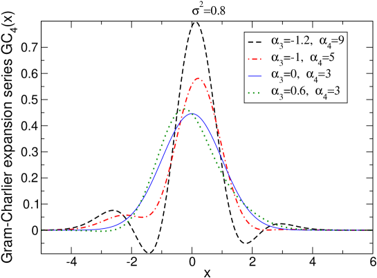
Figure 1: (Color online) Fourth-order symmetrical Gram-Charlier GC₄ distributions for several values of the coefficients $\alpha_{3}$ and $\alpha_{4}$. The full line corresponds to the Gaussian function.

One of the main disadvantages of the Gram-Charlier profile is that in certain circumstances (see Fig. 1), it exhibits some negative features.

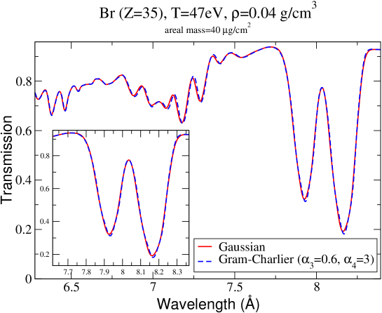
Figure 2: (Color online) Impact of a skewed Gaussian for modeling the opacity lines of a bromine plasma ($T$=47 eV and $\rho$=0.04 g/cm³) in the $2p\rightarrow 3d$ range.

The levels of an electronic configuration verify approximate symmetries, which are called couplings in atomic spectroscopy. In fact, highly asymmetrical line distributions can be found due to some large $G^{1}$ exchange Slater integral. This may happen in arrays of the type $l^{N+1}-l^{N}l^{\prime}$, which are very numerous, because in highly charged ions, the transitions decaying to the ground configuration belong to arrays of this type. The skewness increases steeply as a function of atomic number $Z$ along an iso-electronic sequence. Assuming hydrogenic behaviour, Slater and spin-orbit integrals vary as $Z$ and $Z^{4}$, respectively. It was shown in that case by Bauche et al. [9] that $\alpha_{3}$ behaves roughly as $Z^{6}$. Therefore, asymmetry is particularly pronounced for highly ionized heavy atoms. They can also occur in situations where the spin-orbit interactions are strong enough to split the transition array (medium- or high-$Z$ elements). In the latter case, the asymmetrical shape of the array can also be restored by considering the superposition of symmetrical subarrays. In fact, the impact of skewness is usually small in the conditions typical of the laser experiments conducted to date (density of the order of 0.01 g/cm³ and temperature of a few tens of eV). Fig. 2 displays the comparison between a skewed Gaussian (fourth-order Gram-Charlier (see Eq. (9)) with $\alpha_{3}=0.6$ and $\alpha_{4}=3$ compared to a Gaussian modeling of lines in the case of a bromine plasma at $T$=47 eV and $\rho$=0.04 g/cm³. The spectra are almost indistinguishable.

2.2 Normal Inverse Gaussian

If one wants to take into account the effect of asymmetry, it can be fruitfully done using the NIG (Normal Inverse Gaussian) distribution [10]:

$$\text{NIG}(E)=\frac{\delta\alpha e^{\delta\sqrt{\alpha^{2}-\beta^{2}}+\beta(E-\mu)}}{\delta^{2}+(E-\mu)^{2}}K_{1}(\alpha\sqrt{\delta^{2}+(E-\mu)^{2}}),$$ (10)

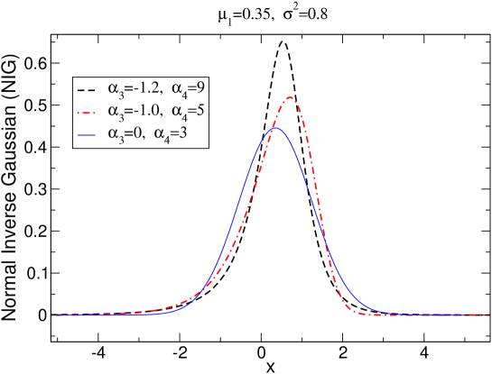
Figure 3: (Color online) Examples of NIG distributions corresponding to different values of the parameters $\alpha$, $\beta$, $\delta$ and $\mu$. The full line corresponds to the Gaussian function.

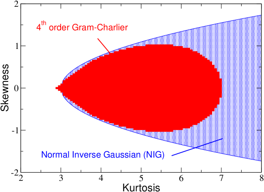
Figure 4: (Color online) Validity domain of the NIG distribution (defined by $|\alpha_{3}|<\sqrt{\frac{3}{5}(\alpha_{4}-3)}$) and positivity domain of the GC₄ distribution.

where $K_{1}$ is a modified Bessel function of the third kind. The four parameters $\alpha$, $\beta$, $\delta$ and $\mu$ are obtained directly from the knowledge of $\mu_{1}$, $\sigma$, $\alpha_{3}$ and $\alpha_{4}$. The corresponding relations as well as the role of the latter parameters can be found in Table 1. Unlike the Gram-Charlier expansion series, the NIG (see Fig. 3) cannot have negative values. Moreover, the validity domain of the NIG is wider than the positivity domain of Gram-Charlier distribution, as shown in Fig. 4. The NIG distribution enables one to model symmetric or asymmetric distributions with possibly long tails in both directions. The tails are much more prominent than in the Gaussian distribution.

2.3 Generalized Gaussian

An interesting choice to study solely the effects of the kurtosis is the generalized Gaussian distribution (GG), defined by:

$$\text{GG}(E)=\frac{\Omega\nu}{\sigma}~{}\frac{e^{-\left|\frac{u}{\lambda}\right|^{\nu}}}{2\lambda~{}\Gamma(\frac{1}{\nu})}\quad\text{with}\quad\lambda=\sqrt{\frac{\Gamma(\frac{1}{\nu})}{\Gamma(\frac{3}{\nu})}},$$ (11)

where $\nu$ is a positive real number, and $\Gamma(x)$ is the ordinary gamma function. The even-order moments of a GG function read:

$$\alpha_{2k}(\text{GG})=\lambda^{2k}~{}\frac{\Gamma(\frac{1+2k}{\nu})}{\Gamma(\frac{1}{\nu})},$$ (12)

whereas the odd-order moments are null, $\alpha_{2k+1}(P)=0$, since the GG is symmetric. The parameter $\nu$ can be obtained by constraining the kurtosis coefficient, and thus solving the equation

$$\alpha_{4}=\frac{\Gamma(1/\nu)\Gamma(5/\nu)}{\Gamma(3/\nu)^{2}}.$$ (13)

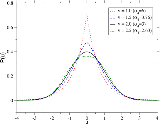
Figure 5: (Color online) Examples of GG distributions (corresponding to different values of the exponent $\nu$).

This distribution is represented in Fig. 5 for several values of the parameter $\nu$ (i.e. for different values of the kurtosis $\alpha_{4}$). The GG function has interesting properties. It is a simple increasing (decreasing) function for $u<0$ ($u>0$), without negative values in contrast with GC series. The Gaussian ($\nu=2$) and the Laplace ($\nu=1$) distributions are special cases of GG functions with a kurtosis coefficient equal to $3$ and $6$, respectively. The discontinuity of the derivative at $u=0$ for $0<\nu\leqslant 1$ disappears with the convolution by another function. The full width at half maximum (FWHM) of a GG function is $2~{}\sigma\lambda~{}(\log 2)^{\frac{1}{\nu}}$, and therefore depends on the distribution itself. For example, the above formula gives $\text{FWHM}=2.35~{}\sigma$ for a Gaussian ($\nu=2$) and $\text{FWHM}=0.98~{}\sigma$ for a Laplace distribution ($\nu=1$). The root of Eq. (13) is fairly well approximated by the fitting function

$$\nu=1.62796\left[\ln(\alpha_{4}-0.783143)\right]^{\frac{0.796349}{\alpha_{4}^{2}}-1}.$$ (14)

2.4 Comparisons of the distributions

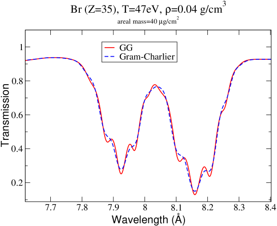
Figure 6: (Color online) Comparison of a transmission spectrum (same as Fig. 2) with a GG_ν=1 profile and a symmetrical GC₄ profile both characterized by the same first four moments (fixing in particular $\alpha_{3}$=0 and $\alpha_{4}$=6).

Fig. 6 displays the comparison of a transmission spectrum (for the same case as Fig. 2) with GG and GC profiles with $\alpha_{3}$=0 and $\alpha_{4}$=6. We observe that both distributions give rise to slightly different spectra, although they are characterized by the same first four moments. The differences are the signature of high-order moments $\alpha_{n}$ ($n>4$). Indeed, the first constained moments fix ipso facto the higher-order unconstrained moments. This can be seen in Table 2, for the transition array $3d^{6}-3d^{5}4p$ in Br XII, which shows the values of $\alpha_{k}$ up to the order $14$ for several distributions. The exact values of the moments are calculated with Cowan’s atomic structure code [11] (routines RCN/RCN2/RCG). They are compared with the values for the GG function, using Eq. (12), with the values for the fourth-order GC series (obtained by setting $c_{k}=0$ for $k\geq 6$) and for the NIG function (requiring $\alpha=0.82$, $\beta=0$, $\delta=3.17$ and $\mu=154.18$). Functions GG, GC₄ and NIG are constrained by the moments of order $k\leq 4$ of the exact distribution. Values for the Gaussian function are also shown. It is observed, for this particular case, that the GG function is slightly closer to the exact values than the other distributions.

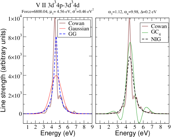
Figure 7: (Color online) Comparison of the line distribution of transition array $3d^{3}4p\rightarrow 3d^{3}4d$ for V II calculated with Cowan’s code, and modeled by a Gaussian, GG, GC₄ and NIG profile. All the distributions are convolved by a Gaussian having a FWHM=0.2 eV.

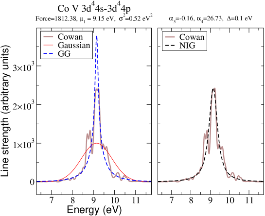
Figure 8: (Color online) Same as Fig. 7 for the transition array $3d^{4}4s\rightarrow 3d^{4}4p$ of Co V with a Gaussian linewidth of FWHM=0.1 eV.

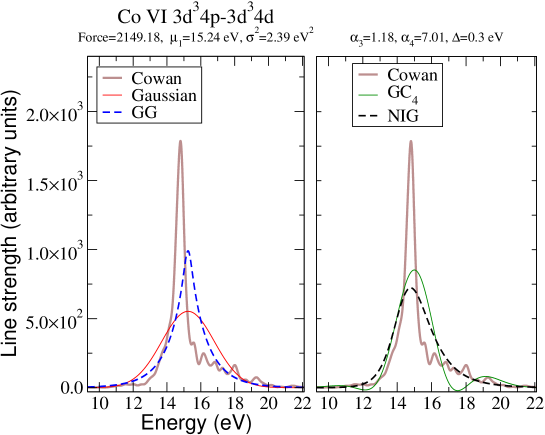
Figure 9: (Color online) Same as Fig. 7 for the transition array $3d^{3}4p\rightarrow 3d^{3}4d$ of Co VI with a Gaussian linewidth of FWHM=0.3 eV.

Transition arrays of the kind $l^{N}l^{\prime}-l^{N}l^{\prime\prime}$ are known to be much sharper than a Gaussian, because of the strong selection rules on the core $l^{N}$. Fig. 7 displays a comparison of the line distribution of transition array $3d^{3}4p\rightarrow 3d^{3}4d$ for V II calculated with Cowan’s code, and modeled by Gaussian, GG, GC₄ and NIG profiles. All the distributions are convolved by a Gaussian having a FWHM=0.2 eV. We can see that the width and heigth of the distribution are not well depicted by the Gaussian. The Gram-Charlier GC₄ distribution has negative features. The GG and NIG distributions are more suited in that case. Fig. 8 displays the same kind of comparisons for the transition array $3d^{4}4s\rightarrow 3d^{4}4p$ of Co V with a Gaussian of FWHM=0.1 eV. The Gram-Charlier GC₄ has not been represented since it exhibits huge non-physical bumps. In that case also the GG and NIG distributions give a better agreement with the exact distribution than the Gaussian. This visual agreement has been confirmed by RMS calculations. Finally, Fig. 9 displays a comparison of the profiles for the transition array $3d^{3}4p\rightarrow 3d^{3}4d$ for Co VI, the distributions being convolved by a Gaussian having a FWHM=0.3 eV. In that case the distribution is asymmetric, and therefore the NIG appears to be the best distribution, but the GG still gives better results that the Gaussian.

We may conclude that the Gaussian is not a good representation for most transition arrays and that GG or NIG are usually better choices than GC when accounting for skewness and/or kurtosis coefficients.

3 Interpretation of recent $2p\rightarrow 3d$ absorption experiments

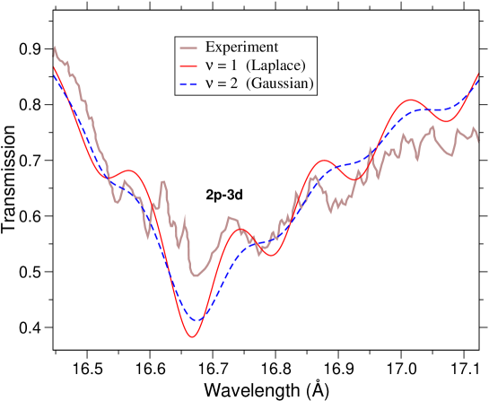
Figure 10: (Color online) Absorption spectrum of iron measured by Chenais-Popovics et al. [12]. The DCA calculations are performed at $T$=20 eV and $\rho$=0.004 g/cm³ assuming either a Gaussian (dashed line) or a GG_ν=1 (full line) profile for the statistical UTA broadening.

Chenais-Popovics et al. [12] measured the absorption of the $2p\rightarrow 3d$ transitions of iron in the range 16.4-17.2 Å. The sample, heated by the thermal radiation of a gold spherical hohlraum, was irradiated by the laser ASTERIX IV. The plasma is assumed to be in local thermodynamic equilibrium (LTE) at a temperature $T=20$ eV and a density $\rho=0.004$ g/cm³. An interpretation using a Detailed Configuration Accounting (DCA) calculation based on SCO code [13] is presented in Fig. 10. It can be seen that the departure from the Gaussian allows one to better reproduce the depth of the successive shoulders in the spectrum which correspond to the transitions $2p_{1/2}\rightarrow 3d_{3/2}$, $2p_{3/2}\rightarrow 3d_{3/2}$ and $2p_{3/2}\rightarrow 3d_{5/2}$ of several ions.

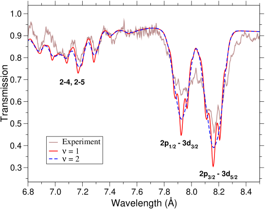
Figure 11: (Color online) Same as Fig. 10 for the NaBr (in the Br range) experiment of Bailey et al. [14] at $T$=47 eV and $\rho$=0.04 g/cm³.

The Z-pinch at Sandia National Laboratory was used by Bailey et al. [14] to measure absorption of NaBr samples. The main purpose of the experiment was to study the $2p\rightarrow 3d$ transitions in bromine ionized into the M-shell. Electron temperature and density, obtained from the analysis of the sodium lines (which are separated from the bromine lines), are respectively $50(\pm 4)$ eV and $3(\pm 1)10^{21}$ cm^-3. The spectral resolution is about $1.5$ eV. The spin-orbit interactions clearly separate the $2p_{1/2}\rightarrow 3d_{3/2}$ and $2p_{3/2}\rightarrow 3d_{5/2}$ structures. Fig. 11 displays the experimental spectrum and the calculated DCA spectra at $T=47$ eV obtained with a Gaussian (dashed curve) or a GG_ν=1 function (full line) for the shape of the transition arrays. Some details of the $2p\rightarrow 3d$ structures, hidden in the Gaussian description, appear clearly in the new modeling and give a much better agreement with the experiment. This provides not only a better identification of the experimental features, but also a possible refinement of the temperature and density diagnostic.

4 The evaluation of high-order moments: a challenging task

4.1 Complexity of the calculation

Moments $\mu_{n}$ defined in Eq. (4) can be expressed in terms of sums involving products of radial integrals. A first difficulty is that the number of terms in that sum increases very rapidly as the order increases. For instance, assuming that the transition array of interest is characterized by $q$ different Slater integrals ($R$) and $r$ different spin-orbit integrals ($\zeta$), the number of terms of the form $\underbrace{R\cdots R}_{\text{n terms}}\underbrace{\zeta\cdots\zeta}_{\text{p terms}}$ is

$$N_{\text{max}}=S_{q}(n)\times S_{r}(p),$$ (15)

where

$$S_{t}(v)=\left(\begin{array}[]{c}\!\!v+t-1\!\!\\ \!\!t-1\!\!\end{array}\right)=\frac{(v+t-1)!}{(t-1)!\;v!}.$$ (16)

Table 3 gives $N_{\text{max}}$ for each kind of product of such integrals and for each of the first four moments $\mu_{n}$, $n$=1, 2, 3 and 4. Obviously, this is a maximum since some of the terms do not exist due to angular-momentum symmetries. In particular, terms of the kind $R\cdots R\zeta$ containing only one $\zeta$ integral are not included since their contribution is zero due to the Landé center-of-gravity rule [3, 11]. One can see that the number of terms increases very fast with respect to the order of the moment. The second difficulty is that the full derivation of each term of the sum is very cumbersome, due to the complex angular-momentum algebra. Uylings has shown [15] that the trace of a $k-$electron operator in the space of the states of an electronic configuration $l^{N}$ is proportional to $\left(\begin{array}[]{c}\!\!4l+2-k\!\!\\ \!\!N-k\!\!\end{array}\right)$. Using second-quantization techniques of Judd [4], one finds that the fourth-order moment of $l^{N+1}\rightarrow l^{N}l^{\prime}$ involves 1- to 10-electron operators and reads therefore

$$\mu_{4}[l^{N+1}\rightarrow l^{N}l^{\prime}]=\sum_{k=1}^{10}\left(\begin{array}[]{c}\!\!4l+2-k\!\!\\ \!\!N+1-k\!\!\end{array}\right)p_{k},$$ (17)

where coefficients $p_{k}$ have to be determined from special cases and symmetry properties (such as complementarity or anti-complementarity). Particular cases are difficult to calculate when dealing with more than two electrons (coefficients of fractional parentage are then required to account for the Pauli exclusion principle). But the calculation is a hard task even with only two electrons ; for instance, considering the simple transition array $l^{2}\rightarrow ll^{\prime}$ (corresponding to $N$=1), one has:

$$\mu_{4}[l^{2}\rightarrow ll^{\prime}]=\sum_{k_{1},k_{2},k_{3},k_{4}}A_{k_{1},k_{2},k_{3},k_{4}}F^{k_{1}}(ll)F^{k_{2}}(ll)F^{k_{3}}(ll)F^{k_{4}}(ll)+\cdots,$$ (18)

with

$$A_{k_{1},k_{2},k_{3},k_{4}}\propto(2-(-1)^{L})[L]\left\{\begin{array}[]{ccc}l&l&k_{1}\\ l&l&L\end{array}\right\}\left\{\begin{array}[]{ccc}l&l&k_{2}\\ l&l&L\end{array}\right\}\left\{\begin{array}[]{ccc}l&l&k_{3}\\ l&l&L\end{array}\right\}\left\{\begin{array}[]{ccc}l&l&k_{4}\\ l&l&L\end{array}\right\},$$ (19)

where $[L]=2L+1$ and $F^{k_{i}}(ll)$ is a direct Slater integral describing electrostatic interactions between two electrons inside orbital $l$. The quantity $A_{k_{1},k_{2},k_{3},k_{4}}$ contains also the $L$-independent product

$$[<l||C^{(k_{1})}||l><l||C^{(k_{2})}||l><l||C^{(k_{3})}||l><l||C^{(k_{4})}||l>]^{2},$$ (20)

where

$$<l||C^{(k)}||l>=(-1)^{l}[l]\left(\begin{array}[]{ccc}l&k&l\\ 0&0&0\end{array}\right),$$ (21)

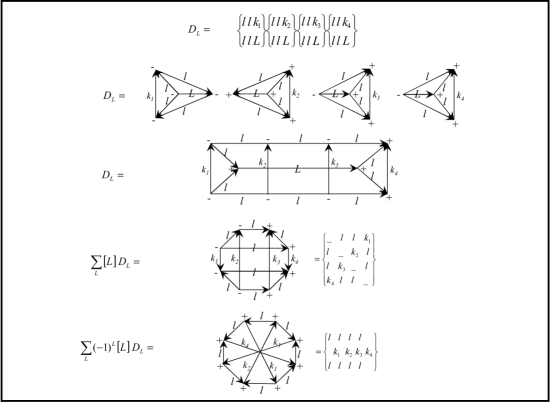
Figure 12: Complexity of the calculation of a simple part of the fourth moment $\mu_{4}$ of the simple transition array $l^{2}\rightarrow ll^{\prime}$ illustrated by graphical methods.

is the reduced matrix element of the spherical function operator $C^{(k)}$, with the phase convention of Ref. [11]. Using the graphical representation of 6-$j$ symbols [16], a compact graph is obtained for the product of four 6-$j$ symbols involved in $A_{k_{1},k_{2},k_{3},k_{4}}$ (see Fig. 12). The summation over $L$ leads to a 12-$j$ symbol of the second kind, and the summation over $L$ with the phase factor $(-1)^{L}$ to a 12-$j$ symbol of the first kind [17]. Therefore, the “direct” calculation of the moments is complicated and the final result would take many pages. However, some algorithms have been proposed in order to evaluate these high-order moments. Karazija et al. [18, 19, 20] expressed the spectral moments by averages of the products of operators and formulated a general group-diagrammatic method for the evaluation of their explicit expressions. Oreg et al. [21] used the fact that the moments reduce to configuration averages of n-boby symmetrical operators (nBSTOs). For that purpose, they introduced the concept of an n-electron minimal configuration, relative to the actual (N-electron) configuration average. Their algorithm uses graphical technique (routine NJGRAF [22]) in order to derive the dependence of the averages on the orbital quantum numbers in terms of closed diagrams.

4.2 Estimation of the kurtosis coefficient

Let us consider the following ideal distribution of line energies and amplitudes [23, 24]:

$$D(\epsilon,a)=\frac{L}{\sqrt{2\pi v}}\exp\left[-\frac{\epsilon^{2}}{2v}\right]\frac{\lambda}{2}\exp[-\lambda|a|],$$ (22)

where $v$ is the unweighted variance of the line energies:

$$v=\frac{1}{L}\sum_{a,b}\left(E_{ab}\right)^{2}-\frac{1}{L^{2}}\left[\sum_{a,b}E_{ab}\right]^{2},$$ (23)

$\epsilon$ is the line energy, $a$ the line amplitude and $L$ the number of lines. The average value of any quantity $q(\epsilon,a)$ is given by

$$<q>=\frac{1}{L}\int\int d\epsilon~{}da~{}D(\epsilon,a)~{}q(\epsilon,a).$$ (24)

Following Ref. [23], the correlation law between the line energies and amplitudes is taken to be

$$v_{a}(\epsilon)=\frac{2}{\lambda^{2}}=\gamma\exp[-\beta|\epsilon|],$$ (25)

where $v_{a}$ is the variance of the line amplitudes, corresponding to the average line strength between two levels. The parameters $\gamma$ and $\beta$ are determined by requiring the conservation of the total strength $S=\sum_{a,b}S_{ab}=L<a^{2}>$ and of the weighted variance $v_{w}$ of the line energies:

$$v_{w}=\frac{1}{S}\sum_{a,b}S_{ab}\left(E_{ab}\right)^{2}-\frac{1}{S^{2}}\left[\sum_{a,b}E_{ab}\right]^{2}=\frac{L}{S}<a^{2}\times\epsilon^{2}>.$$ (26)

The kurtosis is given by

$$\alpha_{4}=\frac{S}{L}\frac{<a^{2}\times\epsilon^{4}>}{<a^{2}\times\epsilon^{2}>^{2}},$$ (27)

which leads to the following expression:

$$\alpha_{4}=\frac{1}{\omega^{2}}[-2+(5+X^{2})\omega],$$ (28)

where $\omega=v_{w}/v$, and $X$ is the root of the following equation:

$$(1+X^{2}-\omega)\exp\left[\frac{X^{2}}{2}\right]\text{erfc}\left[\frac{X}{\sqrt{2}}\right]-\sqrt{\frac{2}{\pi}}X=0.$$ (29)

The energy-amplitude correlation is such that, considering the case where the spin-orbit interaction is weak, the stronger lines are found closer to the center of gravity than the weaker ones. Due to these correlations (propensity rule), the transition array is expected to be sharp. In other words, the variance of the line energies is always smaller when it is calculated with a weight equal to the line strength (see Eq. (26)) than when it is not (see Eq. (23)). Eq. (22) implies that the energy-dependent distribution of line strengths $S(\epsilon)$ (i.e. the shape of the transition array) can be written

$$S(\epsilon)=v_{a}(\epsilon)\frac{L}{\sqrt{2\pi v}}\exp\left[-\frac{\epsilon^{2}}{2v}\right],$$ (30)

which means that, if Eq. (22) is fulfilled, the resulting shape has necessarily a kurtosis between 3 (Gaussian) and 6 (Laplace). Table 4 shows the values of $\alpha_{4}$ estimated from Eq. (28) compared to the exact ones (i.e. calculated from Cowan’s code).

5 Conclusion

The UTA formalism gives the first two moments of the distribution of electric-dipolar lines. It does not contain any assumption as concerns the modeling function. Usually, the chosen distribution is the Gaussian (kurtosis $\alpha_{4}$=3), but detailed calculations using Cowan’s code show that it is often not the most proper distribution, since it does not account for the skewness and kurtosis coefficients. In this article, several other distributions have been studied in an attempt to include the effects of high-order moments. Gram-Charlier expansion series, which consists in a Gaussian multiplied by a linear combination of Hermite polynomials, can have negative values. The Normal Inverse Gaussian function is well suited in order to account for asymmetry and flatness. However, the impact of asymmetry is usually small in the conditions typical of usual photo-absorption experiments, and the Generalized Gaussian function seems to be a good choice in order to account for the specific effect of the kurtosis [25]. With such a modeling, more detailed structures appear in spectra, leading to a better agreement with recent $2p\rightarrow 3d$ absorption experiments and improving in that way the temperature and density diagnostics. The analytical calculation of high-order ($n\geq 3$) moments is possible (see the works of Karazija et al. [18, 19, 20] and Oreg et al. [21]), but difficult. An approximate method, relying on a physically realistic distribution of line amplitudes and energies, has been proposed in order to estimate the kurtosis. The next step will be the calculation of high-order STA (Super Transition Arrays [26]) moments.

Acknowledgements

The authors would like to thank J.E. Bailey, and C. Chenais-Popovics for providing the experimental spectra.

Parameter	Expression	Role
$\alpha$	$\frac{3\sqrt{3\tilde{\alpha}_{4}-4\alpha_{3}^{2}}}{\sigma(3\tilde{\alpha}_{4}-5\alpha_{3}^{2})}$	Tail heaviness
$\beta$	$\frac{3\alpha_{3}}{\sigma(3\tilde{\alpha}_{4}-5\alpha_{3}^{2})}$	Asymmetry
$\delta$	$\frac{3\sigma\sqrt{3\tilde{\alpha}_{4}-5\alpha_{3}^{2}}}{3\tilde{\alpha}_{4}-4\alpha_{3}^{2}}$	Scale parameter
$\mu$	$\mu_{1}-\frac{\delta\alpha_{3}}{\sqrt{3\tilde{\alpha}_{4}-5\alpha_{3}^{2}}}$	Location

Table 1: Parameters of the NIG distribution. The quantity $\tilde{\alpha}_{4}=\alpha_{4}$-3 represents the excess kurtosis.

order	exact	GGν=1.356	GC4	NIG	Gaussian
4	4.15	4.15	4.15	4.15	3
6	33.59	34.73	32.22	38.81	15
8	433.98	466.46	346.10	665.06	105
10	7772	8954	4562	18480	945
12	1.73 $10^{5}$	2.29 $10^{5}$	0.70 $10^{5}$	7.66 $10^{6}$	10395
14	4.52 $10^{6}$	7.45 $10^{6}$	1.22 $10^{6}$	4.46 $10^{7}$	135140

Table 2: Values of the even reduced centered moments $\alpha_{k}$ of several distributions representing the transition array $3d^{6}\rightarrow 3d^{5}4p$ in Br XII. Exact: calculation with Cowan’s code; GG: generalized Gaussian function with $\nu$=1.356; GC₄: fourth-order Gram-Charlier series with $\alpha_{3}$=0 and $\alpha_{4}$=4.15; NIG: Normal Inverse Gaussian with $\alpha$=0.82, $\beta$=0, $\delta$=3.17, $\mu$=154.18.

Order	1	2	3	4
Products involved	$R$	$RR$, $\zeta\zeta$	$RRR$, $R\zeta\zeta$, $\zeta\zeta\zeta$	$RRRR$, $RR\zeta\zeta$, $R\zeta\zeta\zeta$, $\zeta\zeta\zeta\zeta$
Max. number of terms	4	16	54	150

Table 3: Number of terms involving products of radial integrals in the first moments $\mu_{n}$ of transition array $l^{N+1}\rightarrow l^{N}l^{\prime}$.

Transition array	kurtosis
	exact	formula
Fe V $3d^{4}\rightarrow 3d^{3}4p$	$4.1$	$3.8$
Pd VII $4d^{4}\rightarrow 4d^{3}5p$	$4.8$	$4.5$
Sn XXIX $3d^{4}\rightarrow 3d^{3}4p$	$5.9$	$5.1$

Table 4: Estimation of the kurtosis from Eq. (28).

References

- [1] J. Bauche and C. Bauche-Arnoult, Comp. Phys. Rep. 12, 1 (1990).
- [2] G.R. Harrison and M.H. Johnson, Phys. Rev. 38 757 (1931).
- [3] C. Bauche-Arnoult, J. Bauche and M. Klapisch, Phys. Rev. A 20, 2424 (1979).
- [4] B.R. Judd, Second Quantization and Atomic Spectroscopy (Johns Hopkins University, Baltimore, 1967).
- [5] C. Bauche-Arnoult, J. Bauche and M. Klapisch, Phys. Rev. A 25, 2641 (1982).
- [6] C. Bauche-Arnoult, J. Bauche and M. Klapisch, Phys. Rev. A 30, 3026 (1984).
- [7] C. Bauche-Arnoult, J. Bauche and M. Klapisch, Phys. Rev. A 31, 2248 (1985).
- [8] M.G. Kendall and A. Stuart, Advanced Theory of Statistics (Hafner, New York, 1969), Vol. 1.
- [9] J. Bauche, C. Bauche-Arnoult and M. Klapisch, Adv. At. Mol. Phys. 23, 131 (1988).
- [10] O.E. Barndorff-Nielsen, Scandinavian Journal of Statistics 24, 1 (1997).
- [11] R.D. Cowan, The theory of atomic structure and spectra (University of California Press, Berkeley and Los Angeles, 1981).
- [12] C. Chenais-Popovics, H. Merdji, T. Missalla, F. Gilleron, J.C. Gauthier, T. Blenski and, Perrot, M. Klapisch, C. Bauche-Arnoult, J. Bauche, A. Bachelier and K. Eidmann, Astrophys. J. Suppl. Ser. 127, 275 (2000).
- [13] T. Blenski, A. Grimaldi and F. Perrot, J. Quant. Spectrosc. Radiat. Transfer 65, 91 (2000).
- [14] J.E. Bailey, P. Arnault, T. Blenski, G. Dejonghe, O. Peyrusse, J.J. MacFarlane, R.C. Mancini, M. Cuneo, D.S. Nielsen and G.A. Rochau, J. Quant. Spectrosc. Radiat. Transfer 81, 31 (2003).
- [15] P.H.M. Uylings, J. Phys. B: At. Mol. Phys. 17, 2375 (1984).
- [16] A.P. Jucys, Y. Levinson and V. Vanagas, Mathematical Apparatus of the Theory of Angular Momentum (Israel Program for Scientific Translations, Jerusalem, 1964).
- [17] D.A. Varshalovich, A.N. Moskalev and V.K. Khersonskii, Quantum Theory of Angular Momentum (World Scientific, Singapore, 1988).
- [18] R. Karazija, Sums of Atomic Quantities and Mean Characteristics of Spectra (in Russian), Mokslas, Vilnius (1991).
- [19] R. Karazija, Acta Phys. Hungarica 70, 367 (1991).
- [20] R. Karazija and S. Kuas, Lith. J. Phys. 35, 155 (1995).
- [21] J. Oreg, W.H. Goldstein, A. Bar-Shalom and M. Klapisch, J. Comp. Phys. 91, 460 (1990).
- [22] A. Bar-Shalom and M. Klapisch, Comput. Phys. Comm. 50, 375 (1988).
- [23] J. Bauche, C. Bauche-Arnoult, P. Duffy and M. Klapisch, Phys. Rev. A 44, 5707 (1991).
- [24] F. Gilleron, J. Bauche and C. Bauche-Arnoult, J. Phys. B: At. Mol. Opt. Phys. 40, 3057 (2007).
- [25] F. Gilleron, J.-Ch. Pain, J. Bauche and C. Bauche-Arnoult, Phys. Rev. E 77, 026708 (2008).
- [26] A. Bar-Shalom, J. Oreg, W.H. Goldstein, D. Shvarts and A. Zigler, Phys. Rev. A 40, 3183 (1989).