Kinematics and history of the solar neighbourhood revisited
Abstract
We use proper motions and parallaxes from the new reduction of Hipparcos data and Geneva-Copenhagen radial velocities for a complete sample of main-sequence and subgiant stars, and new Padova isochrones to constrain the kinematics and star-formation history of the solar neighbourhood. We rederive the solar motion and the structure of the local velocity ellipsoids. When the principal velocity dispersions are assumed to increase with time as , the index is larger for () than for (). For the three-dimensional velocity dispersion we obtain . We exclude saturation of disc heating after as proposed by Quillen & Garnett (2000). Saturation after combined with an abrupt increase in velocity dispersion for the oldest stars cannot be excluded. For all our models the star-formation rate is declining, being a factor 2–7 lower now than it was at the beginning. Models in which the SFR declines exponentially favour very high disc ages between 11.5 and and exclude ages below as they yield worse fits to the number density and velocity dispersion of red stars. Models in which the SFR is the sum of two declining exponentials representing the thin and thick discs favour ages between 10.5 and with a lower limit of . Although in our models the star-formation rate peaked surprisingly early, the mean formation time of solar-neighbourhood stars is later than in ab-initio models of galaxy formation, probably on account of weaknesses in such models.
keywords:
stars: kinematics - Galaxy: kinematics and dynamics - solar neighbourhood1 Introduction
For the solar neighbourhood we have the most detailed observational data available for any galactic disc. In particular, the distributions within the solar neighbourhood of stellar ages, metallicities and space velocities are keys to deducing how the disc has evolved chemically and dynamically. Work directed at understanding how galaxies have formed and evolved is a major area of contemporary astronomy, and studies of the local disc have an important role to play in this effort. Despite much progress many questions about the evolution of the local disc remain open.
The Hipparcos catalogue provides uniquely useful data for studies of the solar neighbourhood, because the data are homogeneous and of high quality. (1998, hereafter DB98) defined a kinematically unbiased sample of Hipparcos stars and investigated its kinematics, while (2000, hereafter BDB00) used the sample to model the history of star formation and the stochastic acceleration of stars in the disc. In this paper we redefine the sample and then re-work these papers for several reasons.
-
(i)
In a systematic re-reduction of the astrometric data from the Hipparcos satellite, (2007) has been able to diminish significantly the errors for a large number of stars. Using the new data we can enlarge the sample of stars that can be used for modelling.
-
(ii)
BDB00 did not take into account the variation of the scale height of stars with age. Consequently, their conclusions regarding past star-formation rates and rates of stochastic acceleration are wrong. Our analysis remedies this defect.
-
(iii)
From an analysis of the age-velocity dispersion relation in the sample of 189 stars in Edvardsson et al. (1993), Quillen & Garnett (2000) argued that stochastic heating saturates after only and that the velocity dispersion of disc stars increased abruptly ago as a result of a merger. We use our much larger sample to test this conjecture.
-
(iv)
Metallicity and radial-velocity measurements from the Geneva Copenhagen Survey [(2004), hereafter GCS, (2007), hereafter GCS2 and (2008), hereafter GCS3] of F and G dwarfs allow more accurate determinations of the metallicity distribution of disc stars and the three-dimensional velocity dispersions in the corresponding colour interval.
-
(v)
New Padova isochrones have recently been published (, 2008), allowing us to update the input concerning stellar evolution and to improve the modelling of the metallicity distribution.
-
(vi)
A revision of the impact of interstellar reddening on our sample changes some results significantly.
The goal of this paper is the same as that of BDB00: to understand as much of the history of the disc as we can by modelling the large-scale structure of velocity space near the Sun. We do not address the small-scale structure of this space, which was first clearly revealed by the Hipparcos Catalogue through the work of Crezé et al. (1998) and Dehnen (1998).
Section 2 describes our input data. Section 3 updates DB98 by extracting the kinematics of the solar neighbourhood. The work of BDB00 is updated in Section 4, which describes our models, and Section 5, which describes fits of them to the data. Section 6 sums up and compares our results with those of other authors.

2 The Data
2.1 The Sample
We follow the procedure of DB98 to select from the new reduction of the Hipparcos catalogue (, 2007) a kinematically unbiased, magnitude-limited subsample of single stars with high-quality astrometric data.
We determine the apparent magnitude up to which the Hipparcos catalogue is complete (mag), which depends on colour and position on the sky, by comparing the Hipparcos catalogue with the Tycho2 catalogue (, 2000), which is complete to about . For uniformly spaced bins in galactic coordinates and and colour in , we select those stars that are brighter than the second brightest star per bin that is in the Tycho2 but not the Hipparcos catalogue. 44 567 out of the 118 218 Hipparcos stars are single stars that fulfil this criterion. From these stars we further select stars with relative parallax errors of or less. This criterion reduces the sample from 44 567 to 20 360 but ensures that the measured proper motions yield fairly accurate tangential velocities.
Fig. 1 is the colour-magnitude diagram of the sample. For our analysis of the star-formation history, we require a one-to-one relationship between the maximum lifetime of a star and its colour, so we restrict ourselves to main-sequence stars. The lines within which stars are deemed to lie on the main sequence are shown in Fig. 1. The applied CMD cut leaves the possibility for a small number of subgiant stars to enter the sample in the colour range , where the sample might thus be slightly biased towards old stars. The 15 113 stars that lie between these lines comprise our final sample, which is approximately 27% larger than that of DB98. The growth in the sample is most pronounced for blue stars since these tend to be more luminous and distant and therefore have the smallest parallaxes.
GCS have measured radial velocities for 6 918 single F and G dwarfs in our sample. These stars are confined to the colour interval . We use this subsample, for which individual space velocities can be determined, as a control of the results obtained with the main sample.
2.2 Isochrones and Metallicities
The age distribution of main-sequence stars of a given colour must vary with colour because at the blue end of the main sequence all stars must be younger than the short main-sequence lifetime there, while at the red end of the main sequence we see stars that are as old as the disc in addition to recently-formed stars. We use Padova isochrones (, 2008) for masses ranging from 0.15 to to determine the age distribution at each colour. Isochrones depend significantly on the metal content and the Helium abundance , so we have to use several isochrones to simulate the metallicity distribution of the solar neighbourhood. We refer to Section 5.1 for a discussion of the weightings of the isochrones employed and focus on which isochrones to employ.
For the conversion from solar units to and we need to know the solar abundances. (2008) argue that the update of the solar chemical composition by Grevesse et al. (2007) (,) gives rise to several problems and uncertainties and adopt (,) for their solar model. Moreover Chaplin et al. (2007) report that solar models with are inconsistent with the helioseismic data. Since we use the (2008) isochrones, we use their solar composition.
As the measurement of the Helium abundance of a star is difficult, there is little data available on the relationship within the solar neighbourhood. A common, but not undisputed procedure is to assume a linear enrichment law , where is the primordial helium abundance and is the helium-to-metal enrichment ratio. (2003) find for , whereas (2007) using Padova isochrones find that it is doubtful whether a universal linear enrichment law exists. For metallicities similar to the solar one they also find . Unfortunately, this slope when combined with either the traditional values or the new values of Grevesse et al. (2007) is inconsistent with the generally accepted WMAP value (, 2007). Nonetheless we adopt . Table 1 gives the chemical compositions of the isochrones we have employed.
| [Fe/H] | ||
|---|---|---|
| 0.002 | 0.23 | |
| 0.003 | 0.23 | |
| 0.004 | 0.23 | |
| 0.006 | 0.24 | |
| 0.008 | 0.24 | |
| 0.010 | 0.25 | |
| 0.012 | 0.25 | |
| 0.014 | 0.25 | |
| 0.017 | 0.26 | 0.00 |
| 0.020 | 0.27 | 0.08 |
| 0.026 | 0.28 | 0.20 |
| 0.036 | 0.30 | 0.36 |
3 Stellar kinematics
We follow the method of DB98 to calculate the three-dimensional velocity dispersion as a function of colour and use a sliding window in with borders that were adjusted to ensure that there are always 500 stars in a window. Every 100 stars a new point is plotted and thus every fifth point is statistically independent of its predecessors. As explained in DB98, the averages we use here are sensitive to outliers, which have to be rejected. We therefore use an iterative method and reject stars that contribute to more than times the value of the previous iteration.111We use a right-handed coordinate system with increasing towards the Galactic centre and increasing in the direction of Galactic rotation. We use and 6 iterations; 55 stars were rejected.
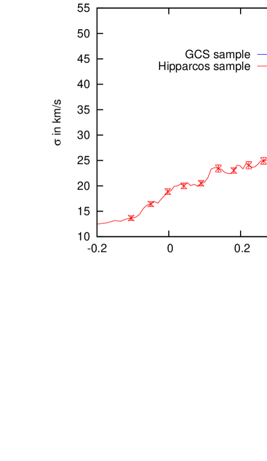
The red points in Fig. 2 show the resulting run of against the mean colour in the sliding windows, with errors in shown for every fifth point. Parenago’s discontinuity – the abrupt end to the increase in velocity dispersion with (, 1950) – is beautifully visible at . We also calculated by combining GCS radial velocities with Hipparcos proper motions, and in Fig. 2 the results are plotted in blue. Where the samples are comparable, there is excellent agreement between the two measurements of . At the upper and lower limits of the GCS sample there are discrepancies because the GCS stars were selected by spectral type, so the bluest GCS bins only contain F stars, while the bins from the Hipparcos sample contain A and F stars and consequently have a lower mean age. For the reddest bins the situation is the same for G and K stars, but this time counterintuitively the pure G star sample has a higher mean age and velocity dispersion – we explain this phenomenon in Section 5.8.
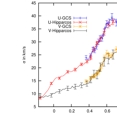
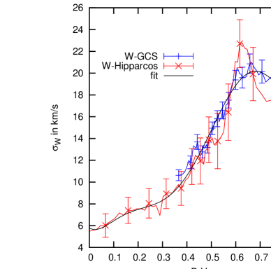
The diagonal elements of the velocity-dispersion tensor are also of interest, as the stochastic acceleration mechanisms at work are anisotropic so each component of the tensor can evolve independently in time (cf. e.g. GCS). Fig. 3 plots and against the mean colour of each bin and Fig. 4 shows . The three-dimensional dispersion is dominated by the radial dispersion , which consequently shows the same features as . The other two components are different, however, and Parenago’s discontinuity is not as beautifully visible in them. For , the dispersion in the direction of rotation, we notice that the slope changes at , but it continues to increase until . Interestingly, in Fig. 4 the values from proper motions (red points) show a significant bump at . A similar bump is visible in DB98 but less strikingly so on account of the larger bins used by DB98. Values of from GCS space velocities have smaller errors and show a less distinctive bump. The GCS error bars on individual components of velocity dispersion are significantly smaller than the corresponding error bars from the larger Hipparcos sample because each Hipparcos star in effect constrains only two components of velocity dispersion. The error bars from the two measurements of overlap, so the results are not inconsistent. The bump originates from a decrease in average age redwards of the discontinuity that we will explain in Section 5.8. In subsequent work we require a functional fit to the data in Fig. 4. Since the radial velocities add valuable additional information, we fit a 5th-order polynomial to the GCS values where these are available, and elsewhere to the proper-motion values. The black curve in Fig. 4 shows the resulting relation.
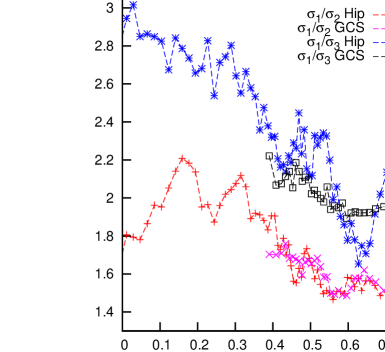
As in DB98, the component of the velocity dispersion tensor is nonzero, implying that the principal axes of are not aligned with our coordinate axes. We diagonalised to find its eigenvalues , the ratios of the square roots of which are plotted in Fig. 5. The ratio (red and magenta) shows a slight decrease with increasing and therefore age, dropping from to through the range . The ratio drops from for the bluest stars to (judging from the GCS sample) for stars redder than Parenago’s discontinuity.
We calculated the sun’s velocity with respect to the LSR as explained in DB98 and found:
| (1) | |||||
These values are consistent with the results of DB98 but our error bars are smaller by per cent. (2007), using a sample of main-sequence stars selected by imposing only an upper limit for relative parallax errors of 10%, found , , in conflict with our values, and , which is consistent with our findings. Since van Leeuwen’s sample extends below the limit to which the Hipparcos sample is photometrically complete, his solar motion may be affected by the kinematic biases that are known to be present in the Hipparcos input catalogue: stars thought be interesting for a variety of reasons were added to the catalogue, and many such stars had come to the attention of astronomers by virtue of a high proper motion.
Using our values for the solar motion and for to calculate the coefficient in Strömberg’s asymmetric drift equation
| (2) |
we find , which is lower than, but still consistent with the result of DB98, and also with the estimated scale length of the Galactic disc (, 2008, §4.8.2(a)).
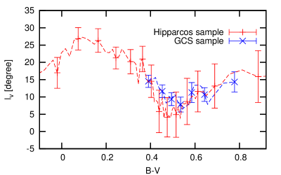
As in DB98, we also calculated the vertex deviation , the angle by which one has to rotate the applied Cartesian coordinate system around its axis to make the velocity dispersion tensor diagonal in the plane. Fig. 6 shows the vertex deviation as a function of colour for bins containing 1000 stars each. As in DB98 the vertex deviation has a minimum at the colour of Parenago’s discontinuity. The displayed errors for the Hipparcos sample are slightly larger than in DB98 because we use smaller bins.
4 Modelling the history of star formation and heating
4.1 Interstellar reddening
For our models, it is important to apply a correction for interstellar reddening to the data because reddening shifts the location of Parenago’s discontinuity, which strongly influences the results of our models for the star formation history. BDB00 corrected the data assuming a linear reddening law, . This law is appropriate for distances of order kiloparsecs, but we live in a low-density bubble within the ISM, so the column density of the ISM and thus the amount of reddening depends on the direction of the line of sight (e.g. , 1995) and for small distances is typically smaller than the mean relation would imply. The code of (1997) allows us to determine the reddening as a function of galactic coordinates , but unfortunately cannot reproduce the results of (2003) or (1998), who find that the reddening within pc of the sun is essentially negligible. Recently GCS2 found that reddening is negligible within pc and between 40 and pc.222The conversion factor between colour systems is (, 1990), so GCS2 find between 40 and pc.
We decided to deredden according to Fig. 4 of (1998). For stars within pc of the midplane and with a distance from the sun between and pc, they find , so we have used
| (3) |
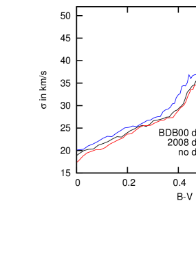
Fig. 7 displays the effect of dereddening on the diagram by comparing data dereddened according to the old and new prescriptions. The binsize used here was 1000 stars and every 200 stars a new data point was added. We see that BDB00 considerably overestimated the effect of reddening.
4.2 Volume completeness
As the velocity dispersion vs. colour diagram alone allows models with a rather large variety of parameters, we use the number of stars per colour interval, , as an additional constraint. Our model of the dynamics will predict , the number of stars of a given colour in a vertical cylinder through the disc that has radius and the sun on its axis. Two points have to be borne in mind when relating this to the observed number density : a) the scale height of stars varies with velocity dispersion and thus colour, and b) the radius of the sphere within which the sample is complete varies with colour.
Assuming the stellar distribution is in equilibrium and neglecting variations with galactic radius, the stellar number density as a function of vertical coordinate , potential and vertical velocity dispersion is
| (4) |
where the normalising factor is to be determined from the observed density . Integrating through the cylinder we have
| (5) |
Integrating through the sphere within which the star count is complete at the given colour we have
where is the completeness radius and is the vertical distance of the sun from the galactic midplane. We now have that the normalising constant is
| (7) |
and on substituting this into equation (5) we obtain the required relation between and the star counts . can be set to any value larger than the largest value of . We set pc (Binney et al., 1997; , 2007) and for we use the polynomial fit shown in Fig. 4. For the potential we use Model 1 of §2.7 of (2008).
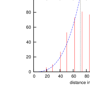
For the determination of we compare the distribution of distances of stars within a radius in a given colour bin to the distribution we would expect, namely
| (8) |
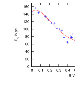
The model density depends on through and we adjust until we have a value for the Kolmogorov–Smirnov (KS) probability that the observed distance distribution at is consistent with the model distribution. These comparisons were made for colour bins that contain 500 stars each. Fig. 8 shows a typical histogram and the corresponding model distribution (8). We finally applied a 5th order polynomial fit to the relation (cf. Fig. 9) and used these radii in eqs. (5) and (7) to relate to . An average of 49 per cent of the stars in a colour bin lie within .
A priori, it is not clear, how to choose the exact limits for the KS probability. Fig. 8 might give rise to doubts concerning the completeness out to the chosen value of . However, if we require higher KS probabilities resulting in lower completeness radii and smaller numbers of stars available for analysis, the results do not change in any significant way. We estimated the errors in the number of stars in the column by varying by 10 per cent around our preferred value and by varying by its -errors. The resulting error was added in quadrature with the Poisson error. This procedure yielded relative errors that varied from below 10 to 25 per cent, but we imposed a lower limit of 15 per cent on the relative error.
To relate all this to BDB00, Fig. 10 shows our selection function (blue) and that of BDB00 (red). One fundamental difference between BDB00 and this work is that we consider a column stretching to , whereas BDB00 considered a sphere with a radius of pc. In BDB00 stars within this volume more luminous than were assumed to be complete, and for less luminous stars the radius of completeness was supposed to decrease as . Hence in Fig. 10 the BDB00 selection function is unity bluer than and then declines linearly. Since we consider a column that extends to infinity, the selection function is always a declining function of luminosity and therefore colour. Hence the most significant difference between the two selection functions is at the blue end where (a) the ability of luminous stars to enter the sample even when far from the plane makes them relatively more numerous in the sample, and (b) the more accurate reduction of the raw Hipparcos data by (2007) has made stars with higher distances available. Even at fainter magnitudes the introduction of the scale-height correction has slightly increased the slope of the selection function, thus depressing the chances of a red star to enter the sample. Consequently, our models have to increase the predicted numbers of red stars in a cylinder relative to the predictions of the BDB00 models.
In summary, roughly half the sample stars contribute to the values of that we model, but all of the sample stars contribute to the modelled values of the velocity dispersions.
4.3 Distribution over age of stars at a given colour
Following BDB00 the distribution of main-sequence stars in a certain volume over age and mass is given by:
| (9) |
where denotes the main-sequence lifetime of a star of initial mass , the initial mass function and ) the star formation rate.
BDB00 used a Salpeter-like power-law IMF and an exponential . They found that the corresponding characterictic parameters and were strongly correlated (see also , 1997). A high, positive value of , i.e. a higher SFR in the past, relatively increases the number of red stars compared to blue stars. This effect can be cancelled by a relatively flat IMF creating more blue stars.
Because of this correlation, we decided to use the IMF of (1993):
| (10) |
The power-law parameter for has the strongest influence on our results and is thus allowed to vary around , the value found by (1993).
With the IMF fixed within a small range, we tested several models for the star formation history:
-
(i)
A simple exponential SFR
(11) -
(ii)
A SFR of the form
(12) with , adding an additional amount of star formation in the early universe.
- (iii)
-
(iv)
A smooth SFR overlaid with a factor varying with time according to Fig. 8 of (2000).
We need the isochrones that were described in Section 2.2 to determine the mass range that can be found in a colour interval at a given time. We cut each isochrone off above the point where it is more luminous than the ZAMS at the same colour. The isochrones provide information only at a limited number of times, so at a desired time one has to interpolate between the next older and next younger isochrones; for the details of this we refer to BDB00.
We can relate to the average distribution over age in a colour interval by
| (14) |
Here the sum is over all mass ranges that lie in the colour interval at age .
4.4 Age–metallicity relation
As we use isochrones with a significantly higher number of metallicities than in BDB00, we are able to include a variation of metallicity with age. As guidelines we use the metallicity distribution published in GCS2 and the age–metallicity relation from the models of (2009a, hereafter SB09a), who are able to reproduce the findings of GCS2 and whose results are also consistent with the age–metallicity relation of (2008).
We find that the GCS2 metallicity distribution has mean and the dispersion . This result is similar to that of (2001), who found that the metallicity distribution for K giants is well represented by a Gaussian with a mean of and a dispersion of . (2001) proposed that the distribution was centred on solar metallicity, which shows that the uncertainty is not negligible. Using a Gaussian representation however omits the metal-poor tail of the GCS2 distribution, which comprises approximately 4% of the total sample and spreads in [Fe/H] from to .
From the models of SB09a we extracted that stars with form only in the first , stars with show a high contribution from the time interval , but also a younger component and stars with started forming after and still form today.
We therefore construct a model that features the following two components:
-
(I)
The ‘thin disc’ component
This component comprises of the model stars and is represented by a Gaussian distribution with the above mentioned mean, so its stars belong to the isochrones with the ten highest metallicities from Table 1. The intrinsic distribution of metallicities will be narrower than the observed one on account of observational errors (cf. Section 5.1). GCS2 conclude that there is no significant change with age in the mean metallicity of solar-neighbourhood stars, so in our models we can consistently use a fit to the current distribution at all times. The models for the star-formation history as described in Section 4.3 and the age refer to this component only.
-
(II)
The ‘low-metallicity’ component
For this component we use only the isochrones with the four lowest metallicities from Table 1:
Stars represented by the isochrones with and with contributions of and have ages ).
Stars represented by with a total contribution of ; two thirds of these have ages ,) and one third has ages ,).
Stars represented by with a contribution of have ages ,). There is also a significant contribution from stars with this metallicity to the ‘thin disc’ component (cf. Section 5.1).
It would seem desirable to assign a velocity dispersion as high as the one of the ‘thick disc’ to this component, however this significantly diminishes the quality of the fits. We thus model both components with a single disc heating rate as described in the following Section and discuss this result in Section 5.7.
4.5 The disc heating rate
We model the velocity dispersion of a group of stars with a known distribution in age by
| (15) |
A simple and often used model (e.g. , 2008, §8.4), that we will mainly consider here is
| (16) |
where and characterise the velocity dispersion at 10 Gyr and at birth and describes the efficiency of stochastic acceleration. However, Quillen & Garnett (2000) argued for saturation of disc heating after and an abrupt increase in velocity dispersion at , which they connected to the formation of the thick disc. Therefore we also consider the following model
| (17) |
where and are the times for the occurrence of saturation and the abrupt increase, and are the saturation velocity dispersions for the thin and the thick disc and and are as above.
Our velocity dispersion data from Section 3 are not for an infinite cylinder, but for a volume-limited Hipparcos sample. As a coeval population heats, it will spread in and the fraction of its stars that contribute to the Hipparcos sphere will drop. So the contribution of this population to the measured dispersion will be less than that of a younger population. We resolve this problem by introducing a weighting factor such that a population’s contribution to the measured dispersion is proportional to
| (18) |
To estimate we consider the conservation of the number of stars born in a certain time interval in the approximation that we can neglect radial mixing. Then, as the population heats and spreads in , its central density drops by a factor , which is given by
| (19) |
The contribution of a population to any sphere around the sun can now be obtained from equations (5) and (7). For our first fit of the model to the data we take . The resulting function is used to determine , a new fit is made and is redetermined. This sequence of operations is rapidly convergent.
The Levenberg–Marquardt non-linear least-squares algorithm (, 1986) is used to minimise the of the fits to the data for and . The parameters adjusted are (for the standard disc heating and SFR model) , , , , and . Data at are discarded for fear that the sample of young stars is kinematically biased. As stated above, the stars are binned in sliding windows of 500 stars, a new one every 100 stars. It might seem desirable to use only statistically independent bins (every fifth bin), but then the results turn out to depend on which subset of bins is used. The compromise used was to use every third bin, which reduces the degradation of the information available about the colours at which dispersions change, at the price of yielding values of that are slightly too low.
| effective weights | ||||||||
|---|---|---|---|---|---|---|---|---|
| ‘thin disc’ comp. | ||||||||
| dex | low high in % | Gyr-1 | Gyr | Gyr | km s-1 | |||
| with low met. tail | ||||||||
| 0 | (0.4, 3.5, 10.0, 16.0, 18.5, 19.5, 16.0, 11.0, 4.4, 0.7) | 0.356 | 0.117 | 12.557 | 0.187 | 55.187 | 1.05 | |
| 0.1 | (0.0, 1.5, 8.0, 17.0, 22.0, 23.0, 17.0, 9.0, 2.5, 0.0) | 0.349 | 0.117 | 12.602 | 0.149 | 55.179 | 1.04 | |
| 0.12 | (0.0, 0.7, 6.0, 17.0, 24.0, 26.0, 17.5, 7.5, 1.3, 0.0) | 0.350 | 0.115 | 12.601 | 0.148 | 55.232 | 1.06 | |
| without low met. tail | ||||||||
| 0 | (0.4, 3.5, 10.0, 16.0, 18.5, 19.5, 16.0, 11.0, 4.4, 0.7) | 0.385 | 0.119 | 12.606 | 0.261 | 57.157 | 0.92 | |
| 0.1 | (0.0, 1.5, 8.0, 17.0, 22.0, 23.0, 17.0, 9.0, 2.5, 0.0) | 0.375 | 0.121 | 11.980 | 0.201 | 57.588 | 0.94 | |
| 0.12 | (0.0, 0.7, 6.0, 17.0, 24.0, 26.0, 17.5, 7.5, 1.3, 0.0) | 0.376 | 0.130 | 11.782 | 0.190 | 57.975 | 1.03 |
5 The results of the fits
As described in BDB00, there are correlations between the parameters which limit the usefulness of the formal errors on the parameters. So we present the results in the following form: we first show the influence of different metallicity weightings on the results and after standardising on a plausible configuration demonstrate the possible range of each parameter by showing the results obtained for fixing it to certain values and leaving the other parameters free. We generally use the total velocity dispersion for our models. The components of are studied in Section 5.5.
5.1 The influence of the metallicity weighting
It is interesting to study how our results depend on the weights we assign to the sequence of the ten isochrones in Table 1 with the highest metallicities, which together represent the ‘thin disc’. As explained in Section 4.4 we consider three values for the observational scatter in [Fe/H]: 0, 0.1 and .
GCS2 give the metallicity distribution of F and G dwarfs near the sun, which is a biased measure of the relative numbers of stars formed with each metallicity because stars of a given mass but different metallicities have different lifetimes and luminosities and therefore probabilities of entering a magnitude-limited sample. Fortunately our model simulates this bias; we simply have to choose the weights of the isochrones such that the contribution of each chemical composition to the modelled magnitude-limited sample agrees with the distribution of metallicities in GCS2. Let be the proportion of the SFR which goes into stars of the th chemical composition. Then the effective weight of this composition is , where and
| (20) |
with the number of stars in the given colour and age range that we would have if the whole disc consisted of stars of the th chemical composition. The are chosen such that after convolution by an appropriate Gaussian distribution of measuring errors the effective weights agree with the metallicity distribution determined by GCS2. The broken curve in Fig. 11 shows the effective weights that correspond to the intrinsic weights of the isochrones, which are shown by the full curve – note that neither curve looks Gaussian because the bins have varying widths. We see that the effective weights are biased towards low metallicities relative to the intrinsic weights .

The adopted metallicity distribution of the ‘thin disc’ component hardly affects the results of the best fit. All parameters and the fit quality are very stable, as is shown in Table 2. As the construction of the low-metallicity component is not straight-forward, we also tested models without this component. The results are also presented in Table 2. For those models the age depends strongly on the metallicity distribution in the sense that the stronger the low-metallicity tail of the distribution, the larger is the recovered value of . Consequently, decreases as we increase our estimate of the errors in the GCS metallicities because the larger the measurement errors, the narrower the distribution of intrinsic metallicities used in the model. The models without a low- component generally show better fit qualities than the two-component models, but broadly speaking all fits are in the same quality range. The old, low-metallicity component is constrained to a relatively small colour interval, whereas for the one-component model, the low-metallicity stars cover all ages and thus a wider colour interval, resulting in a better fit quality. All models with a significant low-metallicity component show very similar ages Gyr.
All the ages in Table 2 are larger than the value obtained by BDB00, principally because the reduction in the estimate of reddening shifts Parenago’s discontinuity to the red, where the average age of stars is higher. The age could be brought down by lowering the helium abundance of the low- isochrones, which would shift the isochrones to redder colours. However, values of significantly below the value of from WMAP would be required to reduce appreciably. Interestingly, (2007) found very low Helium abundances for nearby K-dwarfs using Padova isochrones.
For the following sections we decided to use two-component models with a ‘thin-disc’ metallicity distribution corresponding to measurement errors of and an intrinsic dispersion of .
| fixed | Gyr-1 | Gyr | Gyr | km s-1 | ||
|---|---|---|---|---|---|---|
| 0.250 | 0.141 | 13.000 | 0.001 | 48.257 | 3.78 | |
| 0.300 | 0.119 | 13.000 | 0.001 | 52.615 | 1.29 | |
| 0.349 | 0.117 | 12.602 | 0.149 | 55.179 | 1.04 | |
| 0.420 | 0.112 | 12.281 | 0.486 | 57.449 | 1.19 | |
| 0.500 | 0.120 | 11.605 | 0.978 | 58.963 | 1.58 |
5.2 Varying
Table 3 shows the results of fixing , the exponent in the heating rate, and Fig. 12 shows the fits obtained with the best value () and fits for values of that are just too large () and clearly too small () to be acceptable. For the dependence of on is too flat and we obtain a poor fit to the number counts. Judging from the results, we are able to exclude values of . The fit for is relatively bad for the -data of red stars and the corresponding is too flat for blue stars and too steep just before and around Parenago’s discontinuity. In view also of the large , and the high velocity dispersion at birth (), we conclude that can be excluded.
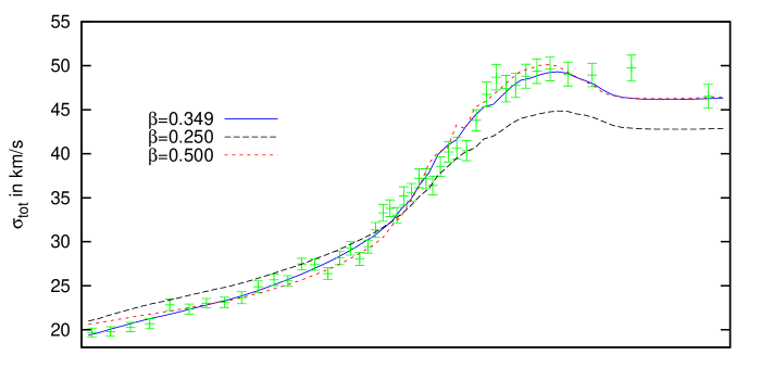
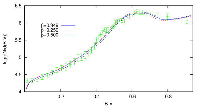
When is increased, the program increases and in an effort to keep the general shape of constant. Since the velocity dispersion of red stars strongly constrains , the increase in is compensated by a decrease in . As the isochrones have limted age ranges, we generally set an upper limit for at 13.0 Gyr. and are relatively stable for the different values of . is only allowed to vary around the (1993) value within the interval .
| Gyr-1 | fixed | Gyr | km s-1 | |||
|---|---|---|---|---|---|---|
| 0.338 | 0.112 | 13.000 | 0.103 | 54.758 | 1.07 | |
| 0.349 | 0.117 | 12.602 | 0.149 | 55.179 | 1.04 | |
| 0.357 | 0.131 | 12.000 | 0.182 | 55.495 | 1.07 | |
| 0.363 | 0.153 | 11.500 | 0.215 | 55.499 | 1.18 | |
| 0.375 | 0.173 | 11.000 | 0.276 | 55.696 | 1.30 | |
| 0.383 | 0.195 | 10.500 | 0.307 | 55.951 | 1.43 | |
| 0.393 | 0.217 | 10.000 | 0.361 | 56.124 | 1.72 | |
| 0.404 | 0.274 | 9.000 | 0.394 | 56.594 | 2.55 |
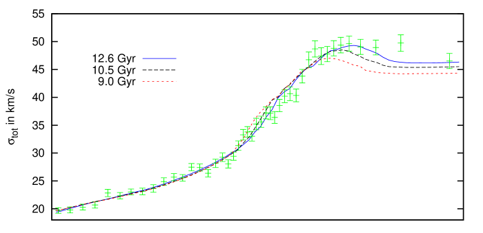
5.3 Varying the age
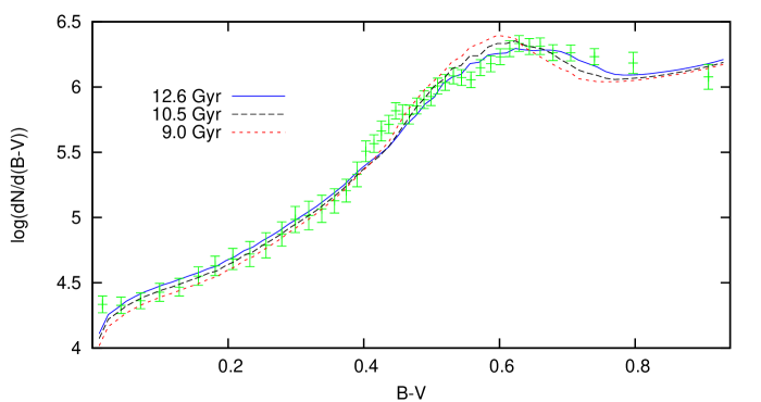
We now examine the effect of optimising the other parameters for fixed age . The favoured ages are higher than in BDB00 and surprisingly large in relation to the accepted age of the universe Gyr. So we fixed at values to see if acceptable younger models could be found. Table 4 shows the results and Fig. 13 displays three fits to the data.
increases with decreasing age as the ratio of old stars to young stars is an important constraint influencing both and . slightly increases with increasing , but is relatively stable. As explained above, low ages are associated with higher values of , and .
Judging from the values of listed in Table 4, ages above are certainly accepted and ages of and lower can be excluded. From Fig. 13 we see that the problem with low ages lies in the reddest bins, in both the and the data. The fit for is definitely unable to represent the data and such low ages have to be excluded. For , is still reasonable but the fit redwards of looks bad. In view of the development of for ages between 11.5 and , we can set a conservative lower age limit .
| Gyr-1 | Gyr | fixed | km s-1 | |||||
|---|---|---|---|---|---|---|---|---|
| 0.00 | 58.90 | 0.317 | 0.117 | 13.000 | 0.000 | 54.200 | 1.11 | |
| 8.14 | 59.46 | 0.329 | 0.116 | 12.673 | 0.030 | 55.056 | 1.09 | |
| 12.65 | 61.82 | 0.349 | 0.117 | 12.602 | 0.149 | 55.179 | 1.04 | |
| 16.04 | 61.36 | 0.416 | 0.119 | 12.096 | 0.500 | 56.944 | 1.17 | |
| 17.27 | 62.22 | 0.462 | 0.119 | 12.020 | 0.800 | 57.483 | 1.39 |
5.4 The velocity dispersion at birth and after
The correlations of the parameters and , which determine the velocity dispersion at birth and for the oldest stars, have already been discussed. only varies within a narrow range, as it is strongly constrained by the observed velocity dispersion redwards of Parenago’s discontinuity. As Table 5 shows, the data allow a wide range of values that correspond to velocity dispersions at birth between 0 and . The effect of this parameter is quite small as the power-law leads to a steep increase of velocity-dispersion within a time small compared to . As the dispersion is already for the bluest bin, the adjustment of the parameters to fit is a minor issue.
| Gyr | km s-1 | |||
|---|---|---|---|---|
| 0.307 | 0.001 | 41.899 | 0.83 | |
| 0.430 | 0.715 | 28.823 | 0.51 | |
| 0.445 | 0.001 | 23.831 | 0.43 |
5.5 Studying the components of
As the results in Section 3 have shown, the three components of show significantly different behaviours: their ratios vary with colour and Parenago’s discontinuity is sharper in some components than in others. Therefore we now seek separate models for the evolution of each eigenvalue of . Since all three models have to satisfy the same data, and the errors on the eigenvalues of are larger than those on , we fix the parameters that describe the star formation history at the best-fit values determined above for , namely , and , and determined for each eigenvalue of only values of the heating parameters, , and . The data for were represented by the polynomial fit shown in Fig. 4.
Table 6 shows the best-fit values of the parameter and . The latter are quite small for and because the formal errors on these components are large. Compared to , is lower, so the heating exponents for the other two components are higher than 0.349. Consequently, and are significantly larger than .
The three values are consistent with Figure 5 in the sense that and both decrease with increasing and thus increasing mean age, and decreases more steeply than , indicating that , which is what we find. However, it has to be mentioned, that because of the rather large interval of acceptable values for encountered in Section 5.2, we cannot exclude .
| fixed | fixed | Gyr | Gyr | km s-1 | ||
|---|---|---|---|---|---|---|
| 0.347 | 0.140 | 12.044 | 0.147 | 54.898 | 1.21 | |
| 0.349 | 0.120 | 12.542 | 0.144 | 55.237 | 1.07 | |
| 0.348 | 0.100 | 13.000 | 0.136 | 55.396 | 1.06 | |
| 0.359 | 0.080 | 13.000 | 0.163 | 56.280 | 1.12 | |
| 0.371 | 0.060 | 13.000 | 0.194 | 57.195 | 1.47 |
| Gyr-1 | Gyr-1 | Gyr | Gyr | km s-1 | ||||||
| 3.0 | 0.346 | 0.095 | 10.022 | 0.132 | 54.968 | 13.2 | 0.21 | 1.19 | ||
| 3.0 | 0.346 | 0.092 | 10.363 | 0.137 | 54.979 | 13.2 | 0.18 | 1.10 | ||
| 3.0 | 0.345 | 0.098 | 10.741 | 0.145 | 54.823 | 10.3 | 0.15 | 1.10 | ||
| 2.0 | 0.349 | 0.085 | 10.233 | 0.147 | 55.145 | 9.7 | 0.21 | 1.18 | ||
| 2.0 | 0.348 | 0.093 | 10.727 | 0.162 | 54.821 | 7.7 | 0.16 | 1.11 | ||
| 2.0 | 0.349 | 0.089 | 11.333 | 0.170 | 54.780 | 7.6 | 0.14 | 1.10 | ||
| 1.0 | 0.350 | 0.073 | 10.604 | 0.170 | 55.058 | 5.6 | 0.22 | 1.18 | ||
| 1.0 | 0.345 | 0.092 | 11.416 | 0.159 | 54.574 | 3.2 | 0.14 | 1.12 |
5.6 Different approaches to the SFR
and are strongly correlated. A high, positive value of , i.e. a higher SFR in the past, increases the number of red stars relative to blue stars. This effect can be cancelled by a relatively flat IMF creating more blue stars. For the investigation of different star formation histories, we thus fixed at the (1993) value of and tested different values of . The best fit in Section 5.3 showed a less steep IMF, so we expect now to find that the model with lowest has a lower value of . Table 7 confirms that this is the case. In all the above Sections, the SFR is decreasing: for the best fit from Section 5.3, it decreases by a factor 4.4 between the beginning of star formation until now. Combining Tables 7 and 4, factors between 2.2 and 6.7 are plausible.
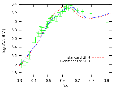
For values of , we had to fix the age to 13.0 Gyr for the reason given above. Our models generally need a large number of old stars. Since stars and older move very slowly in the CMD, it is interesting to ask whether acceptable models with a reduced lower age limit can be obtained by permitting a high SFR early on. Moreover, a short early period of intense star formation is envisaged in the popular proposal that the thick disc formed as a result of a major accretion event ago (e.g. Chiappini et al., 2001).
We thus applied a SFR as described by equation (12). The timescale of the first formation epoch should be small compared to , so we tried , 2 and . The results for different parameters A are displayed in Table 8.
The fraction of solar-neighbourhood stars that belong to the ‘thick disc’ is determined by and . Table 8 gives for each model – observationally (2008) found for their definition of the thick disc, so we used this value as a guidance in adjusting the parameters. We further characterise the scenarios by the ratio of the two terms at the beginning of star formation: . Since models with very small are indistinguishable from standard pure-exponential models, we stopped lowering when reached a value comparable to that of the best-fitting standard model. Significantly, no two-exponential model achieved a lower than the best standard model.
For all scenarios, the parameters , , and are very stable; the disc-heating parameters do not depend significantly on the applied SFR, so there is no need for a further discussion. Compared to its values from Section 5.3, has decreased for the lower ages to compensate for the influence of the added ‘thick disc’ SFR term. The most striking difference is that the favoured ages have decreased by . The best results were achieved for . For the SFR considered here, the lower age limit has to be lowered to .
Fig. 14 compares the fits to the data for the model of Section 5.3 and the model with and . It shows how the intense first period of star formation improves the fits to the data of the red colour bins at lower disc ages.
(2000) argue that the SFR of the solar neighbourhood is very irregular. They also find that the SFR shows an increasing tendency, which is incompatible with our findings. It is however interesting to ask if it is possible to achieve reasonable fits with a smooth SFR overlaid with factor varying in time according to Fig. 8 of (2000). The best fit for this approach has a of 1.44 and is characterised by the following parameters
which are all in the range of acceptable values as determined above. The higher value of results from additional features, which are produced by the varying SFR and which are incompatible with the data. We are, however, not able to exclude a SFR which is not smooth. As Figures 12 and 13 show, there are features in the data that our models are not able to reproduce and which might be produced by epochs of enhanced star formation.
We finally test the SFR described by equation (13), which was proposed by (2007). This SFR increases early on and then decreases. The best-fit model achieves with
In this model the SFR peaked ago and has since decreased by a factor . The fit provided by this is of a similar quality as the best fits with the standard SFR, and the values of all comparable parameters are little changed from when we used the standard SFR.
| Gyr | Gyr | Gyr-1 | Gyr | Gyr | km s-1 | ||||
|---|---|---|---|---|---|---|---|---|---|
| 5.0 | – | 1.0 | 0.588 | 0.114 | 13.000 | 0.845 | 49.468 | 1.69 | |
| 6.0 | – | 1.0 | 0.477 | 0.117 | 13.000 | 0.558 | 50.245 | 1.37 | |
| 7.0 | – | 1.0 | 0.429 | 0.119 | 12.556 | 0.396 | 52.044 | 1.17 | |
| 3.0 | 9.0 | 1.50 | 1.986 | 0.126 | 12.539 | 5.801 | 41.004 | 1.51 | |
| 3.0 | 9.0 | 1.75 | 0.484 | 0.132 | 12.003 | 0.488 | 38.483 | 1.45 | |
| 3.0 | 9.0 | 2.00 | 0.458 | 0.151 | 11.708 | 0.489 | 37.213 | 1.67 | |
| 3.0 | 8.0 | 1.50 | 0.606 | 0.127 | 12.017 | 0.915 | 38.929 | 1.37 | |
| 4.0 | 9.0 | 1.60 | 0.367 | 0.131 | 12.043 | 0.205 | 40.606 | 1.22 | |
| 5.0 | 9.0 | 1.50 | 0.334 | 0.132 | 12.046 | 0.127 | 42.646 | 1.12 |
5.7 Different Approaches to the heating rate
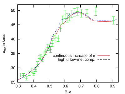
In our models we have so far assumed that the velocity dispersion increases continuously with age. In the context of the Galactic thick disc, an obvious question to ask is what would be the effect of assigning a high velocity dispersion, (, 2004), to the low-metallicity component. Fig. 15 shows that this procedure produces an additional feature in the curve that underlines again the narrow colour interval to which the low-metallicity component is confined. The reason for this is that the thick disk is not only metal-poor and old, but has a more complex structure (, 2009b).
In this context it is also interesting to study whether a saturation of disc heating, or a merger event producing a discontinuity in the time evolution of , or a combination of the two is compatible with the data. We adopt the alternative model (17) of . This model introduces three additional parameters, when heating saturates, when there is a step increase in and , the scale of that increase. Table 9 provides an overview of results obtained by fixing these parameters.
We start by looking at a pure saturation of disc heating () with , and . Intuitively, this model is incompatible with the phenomenon of Parenago’s discontinuity unless , and that is what the results confirm. For we can firmly exclude .
Consider now the proposal of Quillen & Garnett (2000) that , and . Our best fit, obtained with , is shown by the red curve in Fig. 16. The curve of moves from the high to the low side of the data around as a result of two changes in slope at the points marked by arrows; at these points the main-sequence age corresponds to and . This figure and the high given in Table 9 exclude this model.
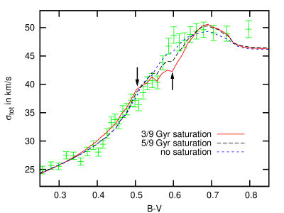
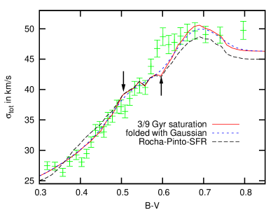
To see whether the unwanted features associated with and could be washed out by an irregular star-formation history rather than the smooth one used in our models, we modelled the data using , , and overlaying our smooth SFR with a factor varying with time according to Fig. 8 of (2000). The resulting fit to the data, shown by the long-dashed line in Fig. 17, is even worse than that shown in Fig. 16. Another possibility is that large errors in (mag) could smooth away the unwanted discontinuities. To test this hypothesis we folded for the (, , 1.75) model with a Gaussian of dispersion. Still the discontinuities did not disappear (short-dashed curve in Fig. 17).
Acceptable models can be found by allowing to approach with corresponding adjustment to . For example, the fit provided by the (, , 1.5) model is shown as the black curve in Fig. 16: the fit to is clearly better than that for (, , 1.75) model and nearly as good as the best fit without saturation (blue curve). Overall one has the impression that models with close to are merely approximating a power-law dependence with an appropriate step.
5.8 Why does decrease redwards of the discontinuity?
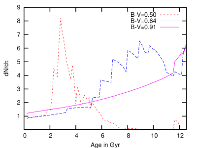
All plots of , whether for models or data, show a counterintuitive decrease in sigma for the reddest bins: the velocity dispersion in our models increases with age, so decreasing implies a decrease in mean age as one moves redwards of the discontinuity. Fig. 18 shows model age distributions at , and . For the reddest colour we see only a smooth increase in numbers with age, reflecting the declining SFR, and a feature at high ages, resulting from the low-metallicty component. At the bluer colours we have strong features. From equation (14) we see that they must reflect wider mass intervals yielding stars of the given colour at a certain time. The explanation for this is that in the vicinity of the turnoff, the isochrones run almost vertically and the colours of stars become nearly independent of mass for a significant range of masses. In Fig. 18 the blue age distribution for shows eight peaks produced in this way, one from each of the eight metallicities used for the ‘thin disk’ component and also a low-metallicity feature at high ages. Because the dominant peaks all lie at ages higher than , they raise the average age of stars in this colour bin above that of the bin for , which contains only stars too low in mass to have reached the turnoff.
6 Conclusion
We have updated the work of DB98 and BDB00 to take advantage of the reworking of the Hipparcos catalogue by (2007), the availability of line-of-sight velocities from the Geneva–Copenhagen survey, and significant improvements to the modelling. The latter include updated isochrones, better treatments of interstellar reddening, the selection function and the age-metallicity relation, and exploration of a wider range of histories of star-formation and stellar acceleration.
We have redetermined the solar motion with respect to the LSR. The new value (eq. 1) is very similar to that of DB98 but has smaller error bars. We have redetermined the structure of the velocity ellipsoid as a function of colour. Again the results differ from those of DB98 mainly in the reduced error bars.
The most striking change in results compared to BDB00 is an increase in the minimum age of the solar neighbourhood . This increase is largely due to an improved treatment of interstellar reddening, which was overestimated by BDB00. Models in which the SFR is fit the data best at and favour ; these models yield a lower age limit of . Models in which the SFR is a double exponential corresponding to the formation of the thick and thin discs favour ages in the range and yield a lower limit of . For either model of the SFR, the lower age limit of BDB00, , can be excluded. Our estimates are in good agreement with the age derived by (2007) and the obtained by SB09a. It is also in agreement with the individual stellar ages of GCS and GCS2, which include a significant fraction of ages between 10 and 15 Gyr. The study of Galactic evolution in a cosmological context by (2001) yields , while that of (2006) yields , our lower limit. Thus there is a considerable body of evidence that the solar neighbourhood started forming a remarkably long time ago.
The strong correlation between the parameters and that characterise the IMF and SFR, which was discussed by (1997) and BDB00, limit what we can say about the IMF and SFR. We use a (1993) IMF and find that the SFR is decreasing: the factor by which it decreases from the beginning of star formation until now is found to lie between and . This conclusion agrees with the findings of (1997) and of (2007), who used a non-exponential time dependence of the SFR, and what we find when the SFR is modelled by a sum of exponentials in time.
Our conclusion regarding the time dependence of the SFR conflicts with the finding of BDB00 that the SFR was essentially flat for a Salpeter IMF because the introduction of variable scale heights decreases the visibility of red stars relative to blue stars, so the models have to predict the existence of a higher fraction of red stars than formerly. It also conflicts with the conclusion of SB09a that the SFR is only mildly decreasing for a Salpeter IMF because in their models many of the old stars in the solar neighbourhood are immigrants from smaller radii while immigration of young stars is negligible. (2001) conclude that the SFR increases in the first and then decreases by a factor 2 until now, while (2000) argue that the Milky Way disc has a generally increasing but very irregular SFR. Neither picture is compatible with our results. There are similar conflicts with the conclusions of (2001) that the SFR is broadly increasing and of (2006) that the SFR increases early on and has been roughly constant over the last .
We can exclude the scenario of Quillen & Garnett (2000) that disc heating saturates after but at the velocity dispersion abruptly increases by a factor of almost 2. However, we are not able to exclude a later saturation of disc heating (after ) that is combined with an abrupt increase in dispersion more recently than ago. Similarly, (2007) find that a saturation at is not excluded and that there is “extremely tentative” evidence of an abrupt feature in the age-velocity dispersion at . Nevertheless, nothing in the data calls for early saturation of disc heating, and scenarios that include it yield worse but formally acceptable fits to the data.
Our favoured value for the exponent that governs the growth of is in perfect agreement with the findings of GCS (0.34) and BDB00 (0.33). Moreover, the value of GCS3 (0.40) is also still in the range allowed by our models. The classical value of (, 1977) yields rather bad fits and has to be regarded as the very upper limit for .
For we find , the same value as in GCS (0.31), but lower than that of GCS3, whose 0.39 is yet not out of range. For we find , which is higher than the GCS and GCS3 values of 0.34 and 0.40. However, had they not ignored their oldest bins of stars, they would have obtained a larger value for . For we find , in good agreement with GCS (0.47) and lower than the value of GCS3 (0.53), but higher than the 0.375 favoured by (2007).
The values and time dependencies of the ratios and plotted in Fig. 5 provide important clues to the still controversial mechanism of stellar acceleration. The original proposal (, 1953) was that acceleration is a result of stars scattering off gas clouds. This process leads to characteristic axial ratios of the velocity ellipsoid. (2008) has recently redetermined these ratios and finds and , both of which are smaller than Fig. 5 implies. This result suggests that scattering by spiral arms, which increases and but not , plays an important role (, 1992). Further work is needed to quantify this statement in the light of Sellwood’s recent work.
Another indication that scattering by clouds is not alone responsible for acceleration is the finding of (2002) that in simulations of disc heating by clouds, , a value that we have excluded. For a disc heated by scattering off a combination of gas clouds and massive black holes in the dark halo (2002) find and , which is excluded by Fig. 5.
It is widely believed that acceleration by spiral arms is responsible for the concentration of solar-neighbourhood stars in the plane (Raboud et al., 1998; Dehnen, 2000; , 2004). (2007) have argued that this concentration undermines the concept of the velocity ellipsoid. However, it remains the case that the velocity dispersions and increase systematically with age and it is not evident that any inconsistency arises from modelling this phenomenon as we do here just because spiral structure accelerates stars in groups rather than individually.
SB09a have recently argued that radial mixing plays an important role in disc heating and causes a higher value of to be measured in the solar neighbourhood than characterises the underlying acceleration process. The origin of this effect is that stars migrate into the solar neighbourhood from small radii where the velocity dispersions are relatively high. Since the fraction of immigrants among the local population increases with stellar age, this effect enhances the velocity dispersion of old stars more than that of young stars, leading to a larger effective value of . Our value for is in good agreement with the prediction of SB09a for a Hipparcos sample.
The models of SB09a are more elaborate than ours not only in that they include radial migration but also in that they include chemical evolution. However, their parameters are determined by fitting to the GCS sample rather than the Hipparcos sample employed here. The current sample covers a wider range of colours and is better defined than the GCS sample. Moreover, SB09a made no attempt to match the kinematics of the GCS sample but assumed the validity of the description of the acceleration process given by BDB00; they confined themselves to the metallicity distribution and Hess diagram of the GCS sample. Ideally one would fit simultaneously the local kinematics, metallicity and Hess diagram. However, given the importance of radial migration implied by the studies of (2008), SB09a and (2009b), such a study would ideally include a more realistic treatment of the integrals of motion than the simple separability of the radial and vertical motions assumed here and by SB09a.
The cosmic SF rate peaked at redshifts (e.g. Ly et al., 2007), which in the concordance cosmology corresponds to look-back times between and . These times are later than the times at which star formation starts in our models, which is also the time at which the local star-formation rate peaked. It is also slightly later than the mean formation times, , of bulges in a recent series of large simulations of galaxy formation (Scannapieco et al., 2009). On the other hand these authors found that the mean formation times of discs at were . The analogous time for the one of our models of the solar neighbourhood is
| (21) | |||||
The models listed in Table 2 yield values of that range between and . These values fall at the upper end of the times obtained by Scannapieco et al. (2009). This overshoot may be connected to the fact that their models have discs that are underweight by almost an order of magnitude; in the models disc formation may be artificially truncated. Thus our results are broadly in agreement with the results of ab-initio simulations of galaxy formation in the concordance cosmology, even though the age of the oldest solar-neighbourhood stars is remarkably large. At least some of these stars will be immigrants from small radii, and if they all are, star-formation will have started later than is implied by our values of . It is currently hard to place a limit on the fraction of the oldest stars that are immigrants because the models of SB09a assume that the disc’s scale length does not increase over time, as is likely to be the case.
Thanks to adaptive optics, gas-rich discs, in which stars are forming exceedingly rapidly, can now be studied observationally at (e.g. Genzel et al., 2008), soon after the oldest solar-neighbourhood stars formed. The discs observed are clumpy and highly turbulent, so it seems more likely that they will turn into bulges than a system as dynamically cold as the solar neighbourhood. Nonetheless, studies of these systems bring us tantalisingly close to the goal of tying together studies of ‘galactic archaeology’ such as ours with observations of galaxies forming in the remote past.
Acknowledgements
We thank Gianpaolo Bertelli for providing us with the latest isochrones and valuable comments on their influence on our models and Ralph Schönrich for valuable discussions. MA thanks Merton College Oxford for its hospitality during the academic year 2007/8.
References
- (1) Bertelli G., Nasi E., 2001, A&A, 121, 1013
- (2) Bertelli G., Girardi L., Marigo P., Nasi E., 2008, A&A, 484, 815
- (3) Binney J.J., Tremaine S., 2008, Galactic Dynamics: Second Edition., Princeton University Press, Princeton
- Binney et al. (1997) Binney J.J., Gerhard O., Spergel D., 1997, MNRAS, 288, 365
- (5) Binney J.J., Dehnen W., Bertelli G., 2000, MNRAS, 318, 658 (BDB00)
- (6) Bensby T., Feltzing S., Lundström I., 2004, A&A, 421, 969
- (7) Casagrande L., Flynn C., Portinari L., Girardi L., Jimenez R., 2007, MNRAS, 382, 1516
- Chaplin et al. (2007) Chaplin W.J., Serenelli A.M., Basu S., Elsworth Y., New R., Verner G.A., 2007, ApJ, 670, 872
- (9) Chiappini C., Matteucci F., Gratton R., 1997, ApJ, 477, 765
- Chiappini et al. (2001) Chiappini C., Matteucci F., Romano D., 2001, ApJ, 554, 1044
- Crezé et al. (1998) Crezé M., Chereul E., Bienamé O., 1998, A&A, 340, 384
- Dehnen (1998) Dehnen W., 1998, AJ, 115, 2384
- Dehnen (2000) Dehnen W., 2000, AJ, 119, 800
- (14) Dehnen W., Binney J.J., 1998, MNRAS, 298, 387 (DB98)
- (15) De Simone R.S., Wu X., Tremaine S., 2004, MNRAS, 350, 627
- Edvardsson et al. (1993) Edvardsson B., Andersen J., Gustafsson E., Lambert D.L., Nissen P.E., Tomkin J., 1993, A&A, 275, 101
- (17) ESA, 1997, The Hipparcos and Tycho Catalogues, ESA-SP 1200
- (18) Frisch P.C., 1995, S.S.Rv., 72, 499
- Genzel et al. (2008) Genzel R., et al., 2008, ApJ, 687, 59
- (20) Girardi L., Salaris M., 2001, MNRAS, 323, 109
- Grevesse et al. (2007) Grevesse N., Asplund M., Sauval A.J., 2007, S.S.Rv., 130, 105
- (22) Hakkila J., Myers J.M., Stidham B.J., Hartmann D.H., 1997, AJ, 114, 2043
- (23) Hänninen J., Flynn C., 2002, MNRAS, 337, 731
- (24) Haywood M., 2001, MNRAS, 325, 1365
- (25) Haywood M., 2008, MNRAS, 388, 1175
- (26) Haywood M., Robin A.C., Crz M., 1997, A&A, 320, 428
- (27) Hernandez X., Avila-Reese V., Firmani C. 2001, MNRAS, 327, 329
- (28) Hg E. et al. 2000, A&A, 355, L27
- (29) Holmberg J., Nordström B., Andersen J., 2007, A&A, 475, 519 (GCS2)
- (30) Holmberg J., Nordström B., Andersen J., 2008, arXiv:0811.3982v1(GCS3)
- (31) Jimenez R., Flynn C., MacDonald J., Gibson B.K., 2003, Sci, 299, 1552
- (32) Jenkins A., 1992, MNRAS, 257, 620
- (33) Joshi Y.C., 2007, MNRAS, 378, 768
- (34) Juric M. et al., 2008, ApJ, 673, 864
- (35) Just A., Jahreiss H., 2007, arXiv:0706.3850
- (36) Kroupa P., Tout C.A., Gilmore G., 1993, MNRAS, 262, 545
- (37) Lallement R., Welsh B.Y., Vergely J.L., Crifo F., Sfeir D., 2003, A&A, 411, 447
- Ly et al. (2007) Ly. C. et al., 2007, ApJ, 657, 738
- (39) Naab T., Ostriker J.P., 2006, MNRAS, 366, 899
- (40) Nordström B. et al., 2004, A&A, 418, 989 (GCS)
- (41) Parenago P.P., 1950, Azh, 27, 150
- (42) Persinger T., Castelaz M.W., 1990, AJ, 100, 1621
- (43) Press W. H., Flannery B. P., Teukolsky A. A., Vetterling W. T, 1986, Numerical Recipes., Cambridge University Press, New York
- Quillen & Garnett (2000) Quillen A.C., Garnett R.G., 2000, astro-ph/0004210v3
- Raboud et al. (1998) Raboud D., Grenon M., Martinet L., Fux R., Udry S, 1998, A&A, 335, 61
- (46) Rocha-Pinto H., Scalo J., Maciel W.J., Flynn C., 2000, A&A, 358, 869
- Scannapieco et al. (2009) Scannapieco C., White S.D.M., Springel V., Tissera P.B., 2009, MNRAS, in press
- (48) Schönrich R., Binney J.J., 2009, MNRAS, in press, arXiv:0809.3006 (SB09a)
- (49) Schönrich R., Binney J.J., 2009, submitted
- (50) Seabroke G.M., Gilmore G. , 2007, MNRAS, 380, 1348
- (51) Sellwood J.A., 2008, in Funes J.G., Corsini E.M., eds, ASP Conf. Ser. Vol. 396, Formation and Evolution of Galaxy Disks. Astron. Soc. Pac., San Francisco, p. 241
- (52) Spergel D.N. et al., 2007, ApJS, 170, 377
- (53) Spitzer L., Schwarzschild M., 1953, ApJ, 118, 106
- (54) Vergely J.L., Freire Ferrero R., Egret D., Köppen J., 1998, A&A, 340, 543
- (55) van Leeuwen F., 2007, Hipparcos, the New Reduction of the Raw Data, Springer Dordrecht
- (56) Wielen R., 1977, A&A, 60, 263