Associated production of Higgs boson and heavy quarks at the LHC: predictions with the $k_{T}$-factorization

Skobeltsyn Institute of Nuclear Physics,
Lomonosov Moscow State University,
119991 Moscow, Russia

Abstract

In the framework of the $k_{T}$-factorization approach, we study the production of Higgs bosons associated with a heavy (beauty or top) quark pair at the CERN LHC collider conditions. Our consideration is based mainly on the off-shell gluon-gluon fusion suprocess $g^{*}g^{*}\to Q\bar{Q}H$. The corresponding matrix element squared have been calculated for the first time. We investigate the total and differential cross sections of $b\bar{b}H$ and $t\bar{t}H$ production taking into account also the non-negligible contribution from the $q\bar{q}\to Q\bar{Q}H$ mechanism. In the numerical calculations we use the unintegrated gluon distributions obtained from the CCFM evolution equation. Our results are compared with the leading and next-to-leading order predictions of the collinear factorization of QCD.

PACS number(s): 12.38.-t, 12.38.Bx

1 Introduction

It is well known that the electroweak symmetry breaking in the Standard Model (SM) of elementary particle interactions is achieved via the Higgs mechanism. This mechanism is responsible for the generation of masses of the gauge ($W^{\pm}$ and $Z^{0}$) bosons as well as leptons and quarks via Yukawa couplings. In the minimal model there are a single complex Higgs doublet, where the Higgs boson $H$ is the physical neutral Higgs scalar which is the only remaining part of this doublet after spontaneous symmetry breaking. In non-minimal models (such as Minimal Supersymmetric Standard Model, MSSM) there are additional charged and neutral scalar Higgs particles. At moment, the Higgs boson is the only missing, undiscovered component of modern particle physics, so that the search for the Higgs boson is of highest priority for particle physics community. It takes important part at the Tevatron experiments and will be one of the main fields of study at the LHC collider [1]. The lower bound on the SM Higgs boson mass from direct searches at the LEP2 energy is $m_{H}>114.4$ GeV [2], while the recent global SM fits to electroweak precision data imply $m_{H}<211$ GeV [3]. The MSSM requires the existence of a scalar Higgs boson lighter than about 130 GeV, so that the possibility of Higgs discovery in the mass range near 115 – 130 GeV seems increasingly likely.

The associated production of a Higgs boson with a heavy (beauty or top) quark pair can play a very important role at high energy hadron colliders. At the LHC, the $t\bar{t}H$ production is an important search channel for Higgs masses below 130 GeV [4–6]. Although the expected cross section is rather small, the signature is quite distinctive. Moreover, analyzing the $t\bar{t}H$ production rate can provide information on the top-Higgs Yukawa coupling [6–9], assuming standard decay branching ratios [6], before model independent precision measurements of this coupling are performed at $e^{+}e^{-}$ colliders [10–12]. The Higgs boson production in association with two beauty quarks is the subject of intense theoretical investigations also [13–15]. In the SM, the coupling of the Higgs to a $b\bar{b}$ pair is suppressed by the small factor $m_{b}/v$, where $v=(\sqrt{2}\,G_{F})^{-1/2}=246$ GeV, implying that the $b\bar{b}H$ production rate is very small at both the Tevatron and the LHC energies. However, in the MSSM this coupling grows with the ratio of neutral Higgs boson vacuum expectation values, $\tan\beta$, and can be significantly enhanced over the SM coupling. Therefore it is one of the most important discovery channels for supersymmetric Higgs particles at the LHC.

From the theoretical point of view, the cross section of Higgs and associated heavy quark pair production at the Tevatron and the LHC is described by the $gg\to Q\bar{Q}H$ and $q\bar{q}\to Q\bar{Q}H$ subprocesses (at the tree level). The leading-order (LO) QCD predictions [14, 15] are plagued by considerable uncertainties due to the strong dependence on the renormalization and factorization scales, introduced by the QCD coupling and the parton (quark and gluon) densities. First estimates of radiative corrections were performed [16] in the so-called ”effective Higgs approximation” (EHA). Recently the calculations of the ${\cal O}(\alpha_{s}^{3})$ inclusive cross section for the $b\bar{b}H$ and $t\bar{t}H$ production have been carried out at next-to-leading order (NLO) [17–20] of QCD. These calculations are based on the complete set of virtual and real ${\cal O}(\alpha_{s})$ corrections to the parton level processes $gg\to Q\bar{Q}H$ and $qq\to Q\bar{Q}H$, as well as the tree level process $(q,\bar{q})g\to Q\bar{Q}H+(q,\bar{q})$. The NLO cross sections are about 20% smaller and about 30% larger than the relevant LO cross sections at the Tevatron and LHC conditions, respectively. It was demonstrated [19, 20] that these high-order QCD corrections greatly reduce the renormalization and factorization scale dependence of LO results and thus stabilize the theoretical predictions.

In the present paper we will study the Higgs and associated heavy (beauty and top) quark pair production using the so-called $k_{T}$-factorization QCD approach [21–24]. This approach is based on the familiar Balitsky-Fadin-Kuraev-Lipatov (BFKL) [25] or Ciafaloni-Catani-Fiorani-Marchesini (CCFM) [26] equations for the non-collinear gluon evolution in a proton. Detailed description of the $k_{T}$-factorization approach can be found, for example, in reviews [27–29]. Here we would like to only mention that the main part of high-order radiative QCD corrections is naturally included into the leading-order $k_{T}$-factorization formalism.

The $k_{T}$-factorization approach has been already applied [30–35] to study the inclusive Higgs production at the Tevatron and LHC conditions. First investigations [30–33] were based on the amplitude for scalar Higgs boson production in the fusion of two off-shell gluons $g^{*}g^{*}\to H$. The corresponding matrix elements have been derived first in [36] using the large $m_{t}$ limit where the effective Lagrangian [37] for the Higgs boson coupling to gluons can be applied. The investigations [30–33] provocated further studies [34, 35] where the off-shell matrix elements of $g^{*}g^{*}\to H$ subprocess have been calculated including finite masses of quarks in the triange loop. It was claimed [35] that the $k_{T}$-factorization approach give us the possibility to estimate the size of unknown collinear high-order corrections.

The starting point of present consideration is the off-shell amplitude of gluon-gluon fusion suprocess $g^{*}g^{*}\to Q\bar{Q}H$. We evaluate the corresponding matrix elements squared for the first time and apply them for investigation of the $b\bar{b}H$ and $t\bar{t}H$ production rates at the LHC energy, $\sqrt{s}=14$ TeV. The quark-antiquark annihilation mechanism, $q\bar{q}\to Q\bar{Q}H$, is expected to be significant only at relatively large $x$, and therefore we can safely take it into accout in the usual leading-order collinear approximation of QCD. In the numerical calculations we will use the unintegrated gluon density in a proton which was obtained [38] from the CCFM equation. Of course, we expect that effects coming from the non-zero gluon virtualities for the associated $b\bar{b}H$ and $t\bar{t}H$ production are not very well prononced even at LHC energies. However, our study is important since it is planned to include the calculated off-shell matrix element $g^{*}g^{*}\to Q\bar{Q}H$ to the Monte-Carlo generator Cascade [39]. We will compare the results obtained in the $k_{T}$-factorization approach with the leading and next-to-leading order predictions of the collinear factorization of QCD.

The outline of our paper is following. In Section 2 we recall shortly the basic formulas of the $k_{T}$-factorization approach with a brief review of calculation steps. We will concentrate mainly on the $g^{*}g^{*}\to Q\bar{Q}H$ subprocess. The evaluation of $q\bar{q}\to Q\bar{Q}H$ contribution is a rather straightforward and therefore will not discussed here (for the reader’s convenience, we only collect the relevant formulas in Appendix). In Section 3 we present the numerical results of our calculations and a discussion. Section 4 contains our conclusions.

2 Theoretical framework

2.1 Kinematics

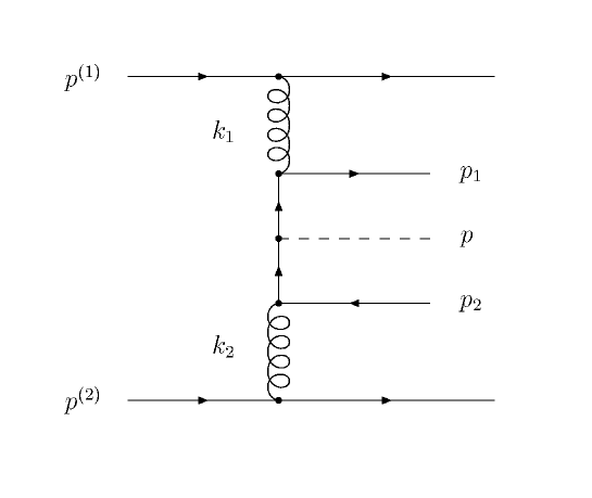
Figure 1: Kinematics of the $g^{*}g^{*}\to Q\bar{Q}H$ process.

We start from the kinematics (see Fig. 1). Let $p^{(1)}$ and $p^{(2)}$ be the four-momenta of the incoming protons and $p$ be the four-momentum of the produced Higgs boson. The initial off-shell gluons have the four-momenta $k_{1}$ and $k_{2}$ and the final quark and antiquark have the four-momenta $p_{1}$ and $p_{2}$ and masses $m_{Q}$, respectively. In the proton-proton center-of-mass frame we can write

$$p^{(1)}={\sqrt{s}}/2\,(1,0,0,1),\quad p^{(2)}={\sqrt{s}}/2\,(1,0,0,-1),$$

where $\sqrt{s}$ is the total energy of the process under consideration and we neglect the masses of the incoming protons. The initial gluon four-momenta in the high energy limit can be written as

$$k_{1}=x_{1}p^{(1)}+k_{1T},\quad k_{2}=x_{2}p^{(2)}+k_{2T},$$

where $k_{1T}$ and $k_{2T}$ are their transverse four-momenta. It is important that ${\mathbf{k}}_{1T}^{2}=-k_{1T}^{2}\neq 0$ and ${\mathbf{k}}_{2T}^{2}=-k_{2T}^{2}\neq 0$. From the conservation laws we can easily obtain the following conditions:

$${\mathbf{k}}_{1T}+{\mathbf{k}}_{2T}={\mathbf{p}}_{1T}+{\mathbf{p}}_{2T}+{\mathbf{p}}_{T},$$

$$x_{1}\sqrt{s}=m_{1T}e^{y_{1}}+m_{2T}e^{y_{2}}+m_{T}e^{y},$$

$$x_{2}\sqrt{s}=m_{1T}e^{-y_{1}}+m_{2T}e^{-y_{2}}+m_{T}e^{-y},$$

where $y$ and $m_{T}$ are the rapidity and the transverse mass of the produced Higgs boson, $p_{1T}$ and $p_{2T}$ are the transverse four-momenta of the final quark and antiquark, $y_{1}$, $y_{2}$, $m_{1T}$ and $m_{2T}$ are their center-of-mass rapidities and transverse masses, i.e. $m_{iT}^{2}=m_{Q}^{2}+{\mathbf{p}}_{iT}^{2}$.

2.2 Off-shell amplitude of the $g^{*}g^{*}\to Q\bar{Q}H$ subprocess

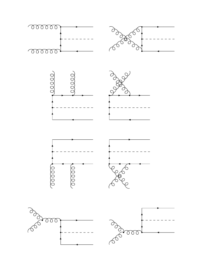
Figure 2: Feynman diagrams which describe the partonic subprocess $g^{*}+g^{*}\to Q\bar{Q}H$ at the leading order in $\alpha_{s}$ and $\alpha$.

There are eight Feynman diagrams (see Fig. 2) which describe the partonic subprocess $g^{*}g^{*}\to Q\bar{Q}H$ at $\alpha\alpha_{s}^{2}$ order. Let $\epsilon_{1}$ and $\epsilon_{2}$ be the initial off-shell gluon polarization vectors and $a$ and $b$ the relevant eight-fold color indices. Then the relevant matrix element can be presented as follows:

$${\cal M}_{1}=g^{2}\,\bar{u}(p_{1})\,t^{a}\gamma^{\mu}\epsilon_{\mu}{\hat{p}_{1}-\hat{k}_{1}+m_{1}\over m_{1}^{2}-(p_{1}-k_{1})^{2}}H{\hat{k}_{2}-\hat{p}_{2}+m_{2}\over m_{2}^{2}-(k_{2}-p_{2})^{2}}t^{b}\gamma^{\nu}\epsilon_{\nu}\,u(p_{2}),$$

$${\cal M}_{2}=g^{2}\,\bar{u}(p_{1})\,t^{b}\gamma^{\nu}\epsilon_{\nu}{\hat{p}_{1}-\hat{k}_{2}+m_{1}\over m_{1}^{2}-(p_{1}-k_{2})^{2}}H{\hat{k}_{1}-\hat{p}_{2}+m_{2}\over m_{2}^{2}-(k_{1}-p_{2})^{2}}t^{a}\gamma^{\mu}\epsilon_{\mu}\,u(p_{2}),$$

$${\cal M}_{3}=g^{2}\,\bar{u}(p_{1})\,t^{a}\gamma^{\mu}\epsilon_{\mu}{\hat{p}_{1}-\hat{k}_{1}+m_{1}\over m_{1}^{2}-(p_{1}-k_{1})^{2}}\,t^{b}\gamma^{\nu}\epsilon_{\nu}{-\hat{p}_{2}-\hat{p}+m_{1}\over m_{1}^{2}-(-p_{2}-p)^{2}}H\,u(p_{2}),$$

$${\cal M}_{4}=g^{2}\,\bar{u}(p_{1})\,t^{b}\gamma^{\nu}\epsilon_{\nu}{\hat{p}_{1}-\hat{k}_{2}+m_{1}\over m_{1}^{2}-(p_{1}-k_{2})^{2}}\,t^{a}\gamma^{\mu}\epsilon_{\mu}{-\hat{p}_{2}-\hat{p}+m_{1}\over m_{1}^{2}-(-p_{2}-p)^{2}}H\,u(p_{2}),$$

$${\cal M}_{5}=g^{2}\,\bar{u}(p_{1})\,H{\hat{p}_{1}+\hat{p}+m_{2}\over m_{2}^{2}-(p_{1}+p)^{2}}\,t^{b}\gamma^{\nu}\epsilon_{\nu}{\hat{k}_{1}-\hat{p}_{2}+m_{2}\over m_{2}^{2}-(k_{1}-p_{2})^{2}}t^{a}\gamma^{\mu}\epsilon_{\mu}\,u(p_{2}),$$

$${\cal M}_{6}=g^{2}\,\bar{u}(p_{1})\,H{\hat{p}_{1}+\hat{p}+m_{2}\over m_{2}^{2}-(p_{1}+p)^{2}}\,t^{a}\gamma^{\mu}\epsilon_{\mu}{\hat{k}_{2}-\hat{p}_{2}+m_{2}\over m_{2}^{2}-(k_{2}-p_{2})^{2}}t^{b}\gamma^{\nu}\epsilon_{\nu}\,u(p_{2}),$$

$${\cal M}_{7}=g^{2}\,\bar{u}(p_{1})\,\gamma^{\rho}C^{\mu\nu\rho}(k_{1},k_{2},-k_{1}-k_{2}){\epsilon_{\mu}\epsilon_{\nu}\over(k_{1}+k_{2})^{2}}f^{abc}t^{c}\times\atop\displaystyle\times{-\hat{p}_{2}-\hat{p}+m_{1}\over m_{1}^{2}-(-p_{2}-p)^{2}}\,H\,u(p_{2}),$$

$${\cal M}_{8}=g^{2}\,\bar{u}(p_{1})\,H\,\epsilon_{\lambda}{\hat{p}_{1}+\hat{p}+m_{2}\over m_{2}^{2}-(p_{1}+p)^{2}}\times\atop\displaystyle\times\gamma^{\rho}C^{\mu\nu\rho}(k_{1},k_{2},-k_{1}-k_{2}){\epsilon_{\mu}\epsilon_{\nu}\over(k_{1}+k_{2})^{2}}f^{abc}t^{c}\,u(p_{2}).$$

In the above expressions $C^{\mu\nu\rho}(k,p,q)$ and $H$ are related to the standard QCD three-gluon coupling and the $H$-fermion vertexes:

$$C^{\mu\nu\rho}(k,p,q)=g^{\mu\nu}(p-k)^{\rho}+g^{\nu\rho}(q-p)^{\mu}+g^{\rho\mu}(k-q)^{\nu},$$

$$H=-{e\over\sin 2\theta_{W}}{m_{Q}\over m_{Z}},$$

where $\theta_{W}$ is the Weinberg mixing angle and $m_{Z}$ is the $Z$-boson mass. The summation on the initial off-shell gluon polarizations is carried out using the BFKL prescription [21–25]:

$$\sum\epsilon^{\mu}(k_{i})\,\epsilon^{\,\nu}(k_{i})={k_{iT}^{\mu}k_{iT}^{\nu}\over{\mathbf{k}}_{iT}^{2}}.$$

This formula converges to the usual expression $\sum\epsilon^{\mu}\epsilon^{\,\nu}=-g^{\mu\nu}$ after azimuthal angle averaging in the $k_{T}\to 0$ limit. The evaluation of the traces in (4) — (11) was done using the algebraic manipulation system Form [40]. We would like to mention here that the usual method of squaring of (4) — (11) results in enormously long output. This technical problem was solved by applying the method of orthogonal amplitudes [41].

The gauge invariance of the matrix element is a subject of special attention in the $k_{T}$-factorization approach. Strictly speaking, the diagrams shown in Fig. 2 are insufficient and have to be accompanied with the graphs involving direct gluon exchange between the protons (these protons are not shown in Fig. 2). These graphs are necessary to maintain the gauge invariance. However, they violate the factorization since they cannot be represented as a convolution of the gluon-gluon fusion matrix element with unintegrated gluon density. The solution pointed out in [23, 24] refers to the fact that, within the particular gauge (15), the contribution from these unfactorizable diagrams vanish, and one has to only take into account the graphs depicted in Fig. 2. We have successfully tested the gauge invariance of the matrix element (4) — (11) numerically.

2.3 Cross section for the $Q\bar{Q}H$ production

According to the $k_{T}$-factorization theorem, the $Q\bar{Q}H$ production cross section via two off-shell gluon fusion can be written as a convolution

$$\sigma(pp\to Q\bar{Q}H)=\int{dx_{1}\over x_{1}}f_{g}(x_{1},{\mathbf{k}}_{1T}^{2},\mu^{2})d{\mathbf{k}}_{1T}^{2}{d\phi_{1}\over 2\pi}\times\atop\displaystyle\times\int{dx_{2}\over x_{2}}f_{g}(x_{2},{\mathbf{k}}_{2T}^{2},\mu^{2})d{\mathbf{k}}_{2T}^{2}{d\phi_{2}\over 2\pi}d{\hat{\sigma}}(g^{*}g^{*}\to Q\bar{Q}H),$$

where $\hat{\sigma}(g^{*}g^{*}\to Q\bar{Q}H)$ is the partonic cross section, $f_{g}(x,{\mathbf{k}}_{T}^{2},\mu^{2})$ is the unintegrated gluon distribution in a proton and $\phi_{1}$ and $\phi_{2}$ are the azimuthal angles of the incoming gluons. The multiparticle phase space $\Pi d^{3}p_{i}/2E_{i}\delta^{(4)}(\sum p^{\rm in}-\sum p^{\rm out})$ is parametrized in terms of transverse momenta, rapidities and azimuthal angles:

$${d^{3}p_{i}\over 2E_{i}}={\pi\over 2}\,d{\mathbf{p}}_{iT}^{2}\,dy_{i}\,{d\phi_{i}\over 2\pi}.$$

Using the expressions (16) and (17) we obtain the master formula:

$$\sigma(pp\to Q\bar{Q}H)=\int{1\over 256\pi^{3}(x_{1}x_{2}s)^{2}}|\bar{\cal M}(g^{*}g^{*}\to Q\bar{Q}H)|^{2}\times\atop\displaystyle\times f_{g}(x_{1},{\mathbf{k}}_{1T}^{2},\mu^{2})f_{g}(x_{2},{\mathbf{k}}_{2T}^{2},\mu^{2})d{\mathbf{k}}_{1T}^{2}d{\mathbf{k}}_{2T}^{2}d{\mathbf{p}}_{1T}^{2}{\mathbf{p}}_{2T}^{2}dydy_{1}dy_{2}{d\phi_{1}\over 2\pi}{d\phi_{2}\over 2\pi}{d\psi_{1}\over 2\pi}{d\psi_{2}\over 2\pi},$$

where $|\bar{\cal M}(g^{*}g^{*}\to Q\bar{Q}H)|^{2}$ is the off-mass shell matrix element squared and averaged over initial gluon polarizations and colors, $\psi_{1}$ and $\psi_{2}$ are the azimuthal angles of the final state quark and antiquark, respectively. We would like to point out again that $|\bar{\cal M}(g^{*}g^{*}\to Q\bar{Q}H)|^{2}$ strongly depends on the nonzero transverse momenta ${\mathbf{k}}_{1T}^{2}$ and ${\mathbf{k}}_{2T}^{2}$. If we average the expression (18) over $\phi_{1}$ and $\phi_{2}$ and take the limit ${\mathbf{k}}_{1T}^{2}\to 0$ and ${\mathbf{k}}_{2T}^{2}\to 0$, then we recover the expression for the $Q\bar{Q}H$ production cross section in the collinear $\alpha\alpha_{s}^{2}$ approximation.

The multidimensional integration in (18) has been performed by means of the Monte Carlo technique, using the routine Vegas [42]. The full C$++$ code is available from the authors upon request.

3 Numerical results

We now are in a position to present our results. According to (18), in the numerical calculations below we have used the CCFM-evolved unintegrated gluon density in a proton, namely set $A0$ [38]. This set is widely discussed in the literature and has been implemented in the Monte-Carlo generator Cascade [39]. As it often done for $Q\bar{Q}H$ production [17–20], we choose the renormalization and factorization scales to be equal: $\mu_{R}=\mu_{F}=\xi(m_{Q}+m_{H}/2)$. In order to investigate the scale dependence of our results we will vary the scale parameter $\xi$ between $1/2$ and 2 about the default value $\xi=1$. As it was proposed in [38], for $\xi=1/2$ and $\xi=2$ we use the $A0-$ and $A0+$ sets of unintegrated gluon densities, respectively. For completeness, we set to $m_{b}=4.75$ GeV, $m_{t}=172$ GeV, $m_{Z}=91.1876$ GeV, $\sin^{2}\theta_{W}=0.23122$ and use the LO formula for the coupling constant $\alpha_{s}(\mu^{2})$ with $n_{f}=4$ active quark flavours at $\Lambda_{\rm QCD}=200$ MeV, such that $\alpha_{s}(M_{Z}^{2})=0.1232$.

We begin the discussion by presenting our numerical results for the associated $b\bar{b}H$ and $t\bar{t}H$ total cross sections as a function of Higgs boson mass for the LHC energy, $\sqrt{s}=14$ TeV. We consider $100<m_{H}<200$ GeV since the production of a Higgs boson in association with a pair of beauty or top quarks at the LHC will play an important role only for relatively light Higgs bosons. The solid histograms in Fig. 3 correspond to the results obtained in the $k_{T}$-factorization approach of QCD with the CCFM-evolved gluon density. The theoretical uncertainties of these predictions are presented by upper and lower dashed histograms. The dash-dotted histograms represent results which were obtained in the standard (collinear) approximation of QCD at LO. The contributions from the quark-antiquark annihilation mechanism, $q\bar{q}\to Q\bar{Q}H$, are shown by the dotted histograms. One can see that using of the $k_{T}$-factorization approach leads to some enhancement of the predicted $b\bar{b}H$ cross section at low $m_{H}$ region (namely $m_{H}<150$ GeV) in respect to the collinear LO QCD results. In the case of $t\bar{t}H$ production, the calculated cross sections in both approaches are very close to each other. It is because the large-$x$ region, namely $x\sim 0.1$, is only covered here and therefore there is practically no effects connected with the small-$x$ physics. It is important that we find our leading-order predictions fully consistent with the corresponding LO results presented in [17–20]. The small visible differense can easily come from the different quark and gluon densities.

In contrast with the NLO QCD results, the $k_{T}$-factorization approach not reduces the strong scale dependence of corresponding LO QCD predictions, which has been pointed out in [17–20]. We conservatively estimate this theoretical uncertainty to be at most of order $40-50$% (see Fig. 3). Such scale dependence is significant, of course, and this fact indicates the necessarity of inclusion of the high-order corrections to the $k_{T}$-factorization formalism. So far the $k_{T}$-factorization is based on the leading-order BFKL or CCFM evolution equations. On the other hand, the kernel of BFKL equation has been calculated already at NLO [45], so that in the small-$x$ regime the $k_{T}$-factorization can be formulated at NLO accuracy also [46]. At moment, this problem is not solved and much more further efforts should be concentrated in this field. We only mention here that the leading-order $k_{T}$-factorization naturally includes the high-energy part of the NLO collinear corrections.

Our predictions for the transverse momentum and rapidity distributions of the Higgs boson as well as associated beauty or top quark $Q$ are shown in Figs. 4 — 7. The distributions on the azimuthal angle distance between the $H$ and $Q$ as well as the $Q$ and $\bar{Q}$ are shown in Figs. 8 and 9, respectively. These calculations were performed using $m_{H}=120$ GeV. The comparison of the $k_{T}$-factorization approach to the collinear one shows the some broadening of the transverse momentum distributions due to extra transverse momentum of the colliding off-shell gluons. Also the $k_{T}$-factorization result shows a more homogeneous spread of the azimuthal angle $\Delta\phi^{H-b}$ distance. At the same time, the cross sections calculated as a function of rapidities $y^{H}$ and $y^{Q}$ as well as the azimuthal angle distributions $d\sigma/d\Delta\phi^{Q-\bar{Q}}$ show a similar behaviour, except for the overall normalization.

To elaborate the difference between the $k_{T}$-factorization approach and the collinear approximation of QCD, we investigate more exclusive observables, like the cross section differential in the total transverse momentum of the $Q\bar{Q}H$ system, $p_{T}^{Q\bar{Q}H}$. In the usual collinear factorization of QCD the effect of intrinsic transverse momenta of the initial gluons can not be described until higher order corrections are taken into account. In the NLO QCD a non-zero $p_{T}^{Q\bar{Q}H}$ is generated by the emission of an additional gluon, while at LO it is always balanced to zero. In the $k_{T}$-factorization formalism, taking into account the non-vanishing initial gluon transverse momentum ${\mathbf{k}}_{T}$ leads to the violation of back-to-back kinematics even at leading order. This effect is clearly illustrated in Fig. 10, where we plot the $b\bar{b}H$ and $t\bar{t}H$ cross sections as a function of $p_{T}^{Q\bar{Q}H}$. Note that only the off-shell gluon-gluon mechanism, $g^{*}g^{*}\to Q\bar{Q}H$, has been taken into account here. The relevant contribution from the quark-antiquark annihilation, $q\bar{q}\to Q\bar{Q}H$, is expected to be almost negligible for $b\bar{b}H$ production and probably can be sizeble for $t\bar{t}H$ one. Keeping in mind that the NLO for this observable is the first non-trivial order, it would be useful to compare the NLO QCD and $k_{T}$-factorization predictions in order to investigate the exact effect of high-order corrections in collinear factorization.

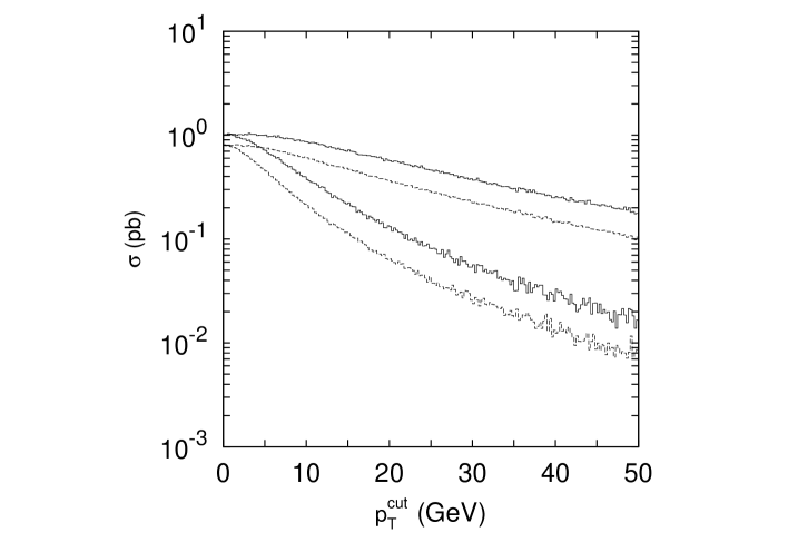
Figure 11: The cross sections for ${b\bar{b}H}$ production with one (upper histograms) or two (lower histograms) high-$p_{T}$ beauty quarks as a function of the minimal $b$-quark transverse momentum $p_{T}^{\rm cut}$ calculated at $m_{H}=120$ GeV and $\sqrt{s}=14$ TeV. The solid and dashed histograms correspond to the results obtained in the $k_{T}$-factorization approach and in the collinear LO approximation, respectively.

In addition, we evaluate the fully exclusive cross section for $b\bar{b}H$ production by requiring that the transverse momentum of one or both final state beauty quarks be large than some $p_{T}^{\rm cut}$ value. This corresponds to an experiment measuring the Higgs decay products along with one or two high $p_{T}$ beauty quark jets that are clearly separated from the beam. In Fig. 11 we illustrate the dependence of these exclusive cross sections on the $p_{T}^{\rm cut}$ parameter. Reducting the $p_{T}^{\rm cut}$ from 50 GeV to zero approximately increases the relevant cross sections by a factors of about 10 and 100, respectively. In the collinear factorization of QCD, if both beauty quarks are required to be produced with $p_{T}>20$ GeV, the NLO corrections reduce the LO predictions, and these corrections are positive if beauty quarks produced at small $p_{T}$ [17]. However, one can see that predictions of the $k_{T}$-factorization approach overestimate the collinear LO results in a wide $p_{T}^{\rm cut}$ range.

Finally, we would like to mention that our $k_{T}$-factorization calculations can be straightforwardly generalized to the case of scalar Higgs bosons of the MSSM by replacing the SM beauty and top quark Yukawa couplings with the corresponding MSSM ones. It is because the off-mass shell matrix element calculated above (see Section 2.2) is proportional to the beauty and top quark Yukawa couplings. In the MSSM, these couplings to the scalar Higgs bosons, $\hat{g}_{QQH}$, are given by a simple rescaling of SM couplings $g_{QQH}$ [47], i.e.

$$\hat{g}_{bbh^{0}}=-{\sin\alpha\over\cos\beta}\,g_{bbh},\quad\hat{g}_{tth^{0}}={\cos\alpha\over\sin\beta}\,g_{tth}\atop\displaystyle\hat{g}_{bbH^{0}}={\cos\alpha\over\cos\beta}\,g_{bbh},\quad\hat{g}_{ttH^{0}}={\sin\alpha\over\sin\beta}\,g_{tth},$$

where $h^{0}$ and $H^{0}$ are the lighter and heavier neutral scalars of MSSM, and $\alpha$ is the angle which diagonalizes the neutral scalar Higgs mass matrix. However, at the NLO level this rescaling is spoiled by one-loop diagrams in which the Higgs boson couples to a closed quark loop. We do not consider supersymmetric-QCD corrections in this paper.

4 Conclusions

We have studied the associated production of Higgs boson and beauty or top quark pair in hadronic collisions at the LHC conditions in the $k_{T}$-factorization approach of QCD. Our consideration is based on the amplitude of off-shell gluon-gluon fusion subprocess $g^{*}g^{*}\to Q\bar{Q}H$. The corresponding off-shell matrix elements have been calculated for the first time. Sizeble contributions from the $q\bar{q}\to Q\bar{Q}H$ mechanism have been taken into account in the LO approximation of collinear QCD.

We have investigated the total and differential cross sections of $b\bar{b}H$ and $t\bar{t}H$ production. In the numerical calculations we have used the unintegrated gluon distributions obtained from the CCFM evolution equation. The comparisons with the leading and next-to-leading order QCD predictions have been made. We demonstrate that the $k_{T}$-factorization approach not reduces the strong scale dependence of collinear LO QCD predictions, pointed out in [17–20]. This fact indicates the importance of the high-order correction within the $k_{T}$-factorization approach. These corrections should be developed and taken into account in the future applications. Finally, we show how our results can be generalized to the scalar Higgs sector of the MSSM. Our calculations is also important for Higgs boson searches where one or two high-$p_{T}$ beauty quarks are tagged in final state.

5 Acknowledgements

We thank S.P. Baranov for the cross-check of matrix elements and very helpful discussions, H. Jung for his encouraging interest and for providing the CCFM code for unintegrated gluon distributions. The authors are very grateful to DESY Directorate for the support in the framework of Moscow — DESY project on Monte-Carlo implementation for HERA — LHC. A.V.L. was supported in part by the grants of the president of Russian Federation (MK-438.2008.2) and Helmholtz — Russia Joint Research Group. Also this research was supported by the FASI of Russian Federation (grant NS-8122.2006.2) and the RFBR fundation (grant 08-02-00896-a).

6 Appendix A

Here we present the compact analytic expressions for the $q\bar{q}\to Q\bar{Q}H$ subprocess. Let us define the four-momenta of the incoming and outgoing quark as $k_{1}$, $k_{2}$, $p_{1}$ and $p_{2}$, respectively. The outgoing quarks have mass $m_{Q}$, i.e. $p_{1}^{2}=p_{2}^{2}=m_{Q}^{2}$. In the formulas below we will neglect the masses of the incoming quarks.

The contribution of the $q\bar{q}\to Q\bar{Q}H$ subrocess to the total $Q\bar{Q}H$ cross section can be easily calculated using the master formula (18). One should only replace the unintegrated gluon densities $f_{g}(x,{\mathbf{k}}_{T}^{2},\mu^{2})$ by the quark ones, perform the summation over initial quark flavours and take the collinear limit. The squared leading-order matrix elements $|\bar{\cal M}(q\bar{q}\to Q\bar{Q}H)|^{2}$ summed over final polarization states and averaged over initial ones can be written as follows:

$$|\bar{\cal M}(q\bar{q}\to Q\bar{Q}H)|^{2}={(4\pi)^{3}\over 72\sin^{2}2\theta_{W}}\left({m_{Q}\over m_{Z}}\right)^{2}\alpha\alpha_{s}^{2}\,\left[{F_{11}\over T_{1}^{2}}+{F_{22}\over T_{2}^{2}}+{F_{12}+F_{21}\over T_{1}T_{2}}\right],$$

where

$$F_{11}=128\,(p_{1}p_{2})(p_{2}k_{1})(p_{2}k_{2})-64\,(p_{1}p_{2})(p_{2}k_{1})(k_{1}k_{2})-64\,(p_{1}p_{2})(p_{2}k_{2})(k_{1}k_{2})-$$

$$64\,(p_{1}p_{2})(k_{1}k_{2})m_{Q}^{2}-64\,(p_{1}k_{1})(p_{2}k_{1})(p_{2}k_{2})+64\,(p_{1}k_{1})(p_{2}k_{1})(k_{1}k_{2})+$$

$$64\,(p_{1}k_{1})(p_{2}k_{2})^{2}+64\,(p_{1}k_{1})(k_{1}k_{2})m_{Q}^{2}-64\,(p_{1}k_{2})(p_{2}k_{1})(p_{2}k_{2})+$$

$$64\,(p_{1}k_{2})(p_{2}k_{1})^{2}+64\,(p_{1}k_{2})(p_{2}k_{2})(k_{1}k_{2})+64\,(p_{1}k_{2})(k_{1}k_{2})m_{Q}^{2}-$$

$$128\,(p_{2}k_{1})(p_{2}k_{2})m_{Q}^{2}+64\,(k_{1}k_{2})m_{Q}^{4}+64\,(k_{1}k_{2})^{2}m_{Q}^{2},$$

$$F_{22}=128\,(p_{1}p_{2})(p_{1}k_{1})(p_{1}k_{2})-64\,(p_{1}p_{2})(p_{1}k_{1})(k_{1}k_{2})-64\,(p_{1}p_{2})(p_{1}k_{2})(k_{1}k_{2})-$$

$$64\,(p_{1}p_{2})(k_{1}k_{2})m_{Q}^{2}-64\,(p_{1}k_{1})(p_{1}k_{2})(p_{2}k_{1})-64\,(p_{1}k_{1})(p_{1}k_{2})(p_{2}k_{2})-$$

$$128\,(p_{1}k_{1})(p_{1}k_{2})m_{Q}^{2}+64\,(p_{1}k_{1})(p_{2}k_{1})(k_{1}k_{2})+64\,(p_{1}k_{1})^{2}(p_{2}k_{2})+$$

$$64\,(p_{1}k_{2})(p_{2}k_{2})(k_{1}k_{2})+64\,(p_{1}k_{2})^{2}(p_{2}k_{1})+64\,(p_{2}k_{1})(k_{1}k_{2})m_{Q}^{2}+$$

$$64\,(p_{2}k_{2})(k_{1}k_{2})m_{Q}^{2}+64\,(k_{1}k_{2})m_{Q}^{4}+64\,(k_{1}k_{2})^{2}m_{Q}^{2},$$

$$F_{12}=F_{21}=-64\,(p_{1}p_{2})(p_{1}k_{1})(p_{2}k_{2})-32\,(p_{1}p_{2})(p_{1}k_{1})(k_{1}k_{2})-64\,(p_{1}p_{2})(p_{1}k_{2})(p_{2}k_{1})-$$

$$32\,(p_{1}p_{2})(p_{1}k_{2})(k_{1}k_{2})-32\,(p_{1}p_{2})(p_{2}k_{1})(k_{1}k_{2})-32\,(p_{1}p_{2})(p_{2}k_{2})(k_{1}k_{2})-$$

$$64\,(p_{1}p_{2})(k_{1}k_{2})m_{Q}^{2}+64\,(p_{1}p_{2})^{2}(k_{1}k_{2})-32\,(p_{1}k_{1})(p_{1}k_{2})(p_{2}k_{1})-$$

$$32\,(p_{1}k_{1})(p_{1}k_{2})(p_{2}k_{2})-32\,(p_{1}k_{1})(p_{2}k_{1})(p_{2}k_{2})+64\,(p_{1}k_{1})(p_{2}k_{1})(k_{1}k_{2})+$$

$$64\,(p_{1}k_{1})(p_{2}k_{2})m_{Q}^{2}+32\,(p_{1}k_{1})(p_{2}k_{2})^{2}+32\,(p_{1}k_{1})(k_{1}k_{2})m_{Q}^{2}+$$

$$32\,(p_{1}k_{1})^{2}(p_{2}k_{2})-32\,(p_{1}k_{2})(p_{2}k_{1})(p_{2}k_{2})+64\,(p_{1}k_{2})(p_{2}k_{1})m_{Q}^{2}+$$

$$32\,(p_{1}k_{2})(p_{2}k_{1})^{2}+64\,(p_{1}k_{2})(p_{2}k_{2})(k_{1}k_{2})+32\,(p_{1}k_{2})(k_{1}k_{2})m_{Q}^{2}+$$

$$32\,(p_{1}k_{2})^{2}(p_{2}k_{1})+32\,(p_{2}k_{1})(k_{1}k_{2})m_{Q}^{2}+32\,(p_{2}k_{2})(k_{1}k_{2})m_{Q}^{2}+64\,(k_{1}k_{2})^{2}m_{Q}^{2},$$

$$T_{1}=(p_{2}k_{1})+(p_{2}k_{2})-(k_{1}k_{2}),\quad T_{2}=(p_{1}k_{1})+(p_{1}k_{2})-(k_{1}k_{2}).$$

Figure 3: The total cross section of associated $b\bar{b}H$ (upper plot) and $t\bar{t}H$ (lower plot) production as a function of Higgs mass at $\sqrt{s}=14$ TeV. The solid histograms correspond to the results obtained in the $k_{T}$-factorization approach of QCD with the CCFM-evolved unintegrated gluon density (set $A0$). The upper and lower dashed histograms represent the scale variations of $k_{T}$-factorization predictions, as it was described in the text. The dash-dotted histograms represent results which were obtained in the standard (collinear) approximation of QCD at LO. The contributions from the quark-antiquark annihilation mechanism (multiplied by a factor of $100$ in the case of $b\bar{b}H$ production) are shown by the dotted histograms.

Figure 4: The transverse momentum distributions $d\sigma/dp_{T}^{H}$ of associated $b\bar{b}H$ (upper plot) and $t\bar{t}H$ (lower plot) production calculated at $m_{H}=120$ GeV and $\sqrt{s}=14$ TeV. Notation of the histograms is the same as in Fig. 3.

Figure 5: The transverse momentum distributions $d\sigma/dp_{T}^{Q}$ of associated $b\bar{b}H$ (upper plot) and $t\bar{t}H$ (lower plot) production calculated at $m_{H}=120$ GeV and $\sqrt{s}=14$ TeV. Notation of the histograms is the same as in Fig. 3.

Figure 6: The rapidity distributions $d\sigma/dy^{H}$ of associated $b\bar{b}H$ (upper plot) and $t\bar{t}H$ (lower plot) production calculated at $m_{H}=120$ GeV and $\sqrt{s}=14$ TeV. Notation of the histograms is the same as in Fig. 3.

Figure 7: The rapidity distributions $d\sigma/dy^{Q}$ of associated $b\bar{b}H$ (upper plot) and $t\bar{t}H$ (lower plot) production calculated at $m_{H}=120$ GeV and $\sqrt{s}=14$ TeV. Notation of the histograms is the same as in Fig. 3.

Figure 8: The azimuthal angle distributions $d\sigma/d\Delta\phi^{H-Q}$ of associated $b\bar{b}H$ (upper plot) and $t\bar{t}H$ (lower plot) production calculated at $m_{H}=120$ GeV and $\sqrt{s}=14$ TeV. Notation of the histograms is the same as in Fig. 3.

Figure 9: The azimuthal angle distributions $d\sigma/d\Delta\phi^{Q-\bar{Q}}$ of associated $b\bar{b}H$ (upper plot) and $t\bar{t}H$ (lower plot) production calculated at $m_{H}=120$ GeV and $\sqrt{s}=14$ TeV. Notation of the histograms is the same as in Fig. 3.

Figure 10: The transverse momentum distributions $d\sigma/dp_{T}^{Q\bar{Q}H}$ of associated $b\bar{b}H$ (upper plot) and $t\bar{t}H$ (lower plot) production calculated at $m_{H}=120$ GeV and $\sqrt{s}=14$ TeV. The off-shell gluon-gluon fusion mechanism is only taken into account.

References

-
[1]
ATLAS Collaboration, Technical Design Report, CERN/LHCC/99-14, 1999;
CMS Collaboration, Technical Proposal, CERN/LHCC/94-38, 1994. - [2] LHWG Note/2002-03, 2002.
- [3] LEPEWWG/2003-01, 2003.
- [4] ATLAS Collaboration, CERN/LHCC/99-15, 1999.
- [5] E. Richter-Was and M. Sapinski, Acta Phys. Pol. B 30, 1001 (1999).
- [6] M. Beneke et al., Report No. CERN 2000-04.
- [7] D. Zeppenfeld, R. Kinnunen, A. Nikitenko, and E. Richter-Was, Phys. Rev. D 62, 013009 (2000).
- [8] A. Belyaev and L. Reina, JHEP 08, 041 (2002).
- [9] F. Maltoni, D. Rainwater, and S. Willenbrock, Phys. Rev. D 66, 034022 (2002).
- [10] A. Djouadi, J. Kalinowski, and P.M. Zerwas, Z. Phys. C 54, 255 (1992).
- [11] S. Dittmaier, M. Kramer, Y. Liao, M. Spira, and P.M. Zerwas, Phys. Lett. B 441, 383 (1998).
- [12] S. Dawson and L. Reina, Phys. Rev. D 59, 054012 (1999).
- [13] R. Raitio and W.W. Wada, Phys. Rev. D 19, 941 (1979).
- [14] J.N. Ng and P. Zakarauskas, Phys. Rev. D 29, 876 (1984).
- [15] Z. Kunszt, Nucl. Phys. B 247, 339 (1984).
- [16] S. Dawson and L. Reina, Phys. Rev. D 57, 5851 (1998).
- [17] S. Dittmaier, M. Kramer, and M. Spira, Phys. Rev. D 70, 074010 (2004).
- [18] S. Dawson, C.B. Jackson, L. Reina, and D. Wackeroth, Phys. Rev. D 69, 074027 (2004).
- [19] W. Beenakker, S. Dittmaier, M. Kramer, B. Plumper, M. Spira, and P.M. Zerwas, Phys. Rev. Lett. 87, 201805 (2001).
- [20] S. Dawson, C.B. Jackson, L.H. Orr, L. Reina, and D. Wackeroth, Phys. Rev. D 68, 034022 (2003).
- [21] V.N. Gribov, E.M. Levin, and M.G. Ryskin, Phys. Rep. 100, 1 (1983).
- [22] E.M. Levin, M.G. Ryskin, Yu.M. Shabelsky, and A.G. Shuvaev, Sov. J. Nucl. Phys. 53, 657 (1991).
- [23] S. Catani, M. Ciafoloni, and F. Hautmann, Nucl. Phys. B 366, 135 (1991).
- [24] J.C. Collins and R.K. Ellis, Nucl. Phys. B 360, 3 (1991).
-
[25]
E.A. Kuraev, L.N. Lipatov, and V.S. Fadin, Sov. Phys. JETP 44, 443 (1976);
E.A. Kuraev, L.N. Lipatov, and V.S. Fadin, Sov. Phys. JETP 45, 199 (1977);
I.I. Balitsky and L.N. Lipatov, Sov. J. Nucl. Phys. 28, 822 (1978). -
[26]
M. Ciafaloni, Nucl. Phys. B 296, 49 (1988);
S. Catani, F. Fiorani, and G. Marchesini, Phys. Lett. B 234, 339 (1990);
S. Catani, F. Fiorani, and G. Marchesini, Nucl. Phys. B 336, 18 (1990);
G. Marchesini, Nucl. Phys. B 445, 49 (1995). - [27] B. Andersson et al. (Small- Collaboration), Eur. Phys. J. C 25, 77 (2002).
- [28] J. Andersen et al. (Small- Collaboration), Eur. Phys. J. C 35, 67 (2004).
- [29] J. Andersen et al. (Small- Collaboration), Eur. Phys. J. C 48, 53 (2006).
- [30] A. Gawron and J. Kwiecinski, Phys. Rev. D70, 014003 (2004).
- [31] H. Jung, Mod. Phys. Lett. A 19, 1 (2004).
- [32] G. Watt, A.D. Martin, and M.G. Ryskin, Phys. Rev. D 70, 014012 (2004); Erratum: ibid. D70, 079902 (2004).
- [33] A.V. Lipatov and N.P. Zotov, Eur. Phys. J. C 44, 559 (2005).
- [34] R.S. Pasechnik, O.V. Teryaev, and A. Szczurek, Eur. Phys. J. C 47, 429 (2006).
- [35] S. Marzani, R.D. Ball, V. Del Duca, S. Forte, and A. Vicini, Nucl. Phys. B 800, 128 (2008).
- [36] F. Hautmann, Phys. Lett. B 535, 159 (2002).
- [37] V. Del Duca, W. Kilgore, C. Olear, C. Schmidt, and D. Zeppenfeld, Nucl. Phys. B 616, 367 (2001); Phys. Rev. D 67, 073003 (2003).
- [38] H. Jung, arXiv:hep-ph/0411287.
-
[39]
H. Jung, Comput. Phys. Commun. 143, 100 (2002);
H. Jung and G.P. Salam, Eur. Phys. J. C 19, 351 (2001). - [40] J.A.M. Vermaseren, ”Symbolic Manipulation with FORM”, published by Computer Algebra Nederland, Kruislaan 413, 1098, SJ Amsterdaam, 1991; ISBN 90-74116-01-9.
-
[41]
R.E. Prange, Phys. Rev. 110, 240 (1958);
S.P. Baranov, Phys. Atom. Nucl. 60, 1322 (1997). - [42] G.P. Lepage, J. Comput. Phys. 27, 192 (1978).
-
[43]
M. Glück, E. Reya, and A. Vogt, Phys. Rev. D 46, 1973 (1992);
M. Glück, E. Reya, and A. Vogt, Z. Phys. C 67, 433 (1995). - [44] H.L.Lai et al. (CTEQ Collaboration), Eur. Phys. J. C 12, 375 (2000).
-
[45]
V.S. Fadin and L.N. Lipatov, Phys. Lett. B 429, 127 (1998);
M. Ciafaloni and G. Gamici, Phys. Lett. B 430, 349 (1998). - [46] J. Bartels, A. Sabio Vera, and F. Schwennsen, JHEP 0611, 051 (2006).
-
[47]
J.F. Gunion and H.E. Haber, Nucl. Phys. B 272, 1 (1982);
J.F. Gunion, H.E. Haber, G.L. Kane, and S. Dawson, ”The Higgs Hunter’s Guide”, SCIPP-89/13.