Spin-glass and other random models

Aligning graphs and finding substructures by a cavity approach

Abstract

We introduce a new distributed algorithm for aligning graphs or finding substructures within a given graph. It is based on the cavity method and is used to study the maximum-clique and the graph-alignment problems in random graphs. The algorithm allows to analyze large graphs and may find applications in fields such as computational biology. As a proof of concept we use our algorithm to align the similarity graphs of two interacting protein families involved in bacterial signal transduction, and to predict actually interacting protein partners between these families.

Over the last decade, the use of graphs for the description of relations between components of complex systems has become increasingly popular [1]. However, most part of the current literature concentrates on (computationally accessible) local characteristics like node degrees, whereas the full exploitation of more global properties of large networks remains frequently elusive due to their inherent algorithmic complexity. Most often studying global properties requires solving NP-hard problems or even harder problems if some form of uncertainty or lack of information is included in the definition of the problem. In both cases heuristic algorithms need to be developed. Specific examples, covered by this article, include the comparison of two different networks, the so-called graph-alignment problem (GA) [2, 3, 4], and the sub-graph isomorphism (SGI), as a particular case of which we consider the widely studied maximum-clique problem [5, 6, 7].

Recently, there has been a lot of interest in distributed algorithms to deal with optimization problems over networks. In the context of statistical physics a new generation of algorithms has been developed (e.g. [8, 9]) that have shown promising performance on several applications (for a review, see [10]). These techniques are based on the so called cavity method and are known as message-passing (MP) algorithms. They are fully distributed and easy to run on parallel machines. A recent result in this framework is an algorithm for finding a connected sub-graph of a given graph which optimizes a given factorized cost function [11].

Here we aim at making a step forward by introducing new techniques for SGI and GA. We develop two alternative MP strategies and test their performance on three sample problems. The first two are well-defined theoretical benchmarks, where our results can be compared to rigorous bounds: (i) the maximum-clique problem in random graphs for the SGI problem; and (ii) the alignment of two random graphs of controlled similarity. The third sample problem is thought as a proof-of-concept application in computational biology: We study (iii) the alignment of the similarity networks of two interacting protein-domain families involved in bacterial signal transduction, to identify actual signaling pathways. This case, involving large networks of $>$2500 nodes, exploits co-evolutionary processes between interacting proteins to identify interaction partners [12].

The model — Both problems, SGI and GA, can be put into the common framework of matching two graphs of possibly different size. Let $G=(V,E,w)$ and $G^{\prime}=(V^{\prime},E^{\prime},w^{\prime})$ be two weighted graphs with nodes $V,V^{\prime}$, edges $E,E^{\prime}$ and edge weights $w,w^{\prime}$. In the applications shown in this letter, weights are non-negative, but this is not a necessary condition for the applicability of the message-passing algorithms. In the case of unweighted graphs, we assume $w$ and $w^{\prime}$ to describe the adjacency matrices, i.e. weights are one if an edge is present between two vertices, and zero else. Further more we denote the node number by $N=|V|$ ($N^{\prime}=|V^{\prime}|$), and the edge number by $M=|E|$ ($M^{\prime}=|E^{\prime}|$). Neighbors of a node $i$ are assembled in $\partial i$. To facilitate notation, primed quantities (in particular node indices) will always refer to $G^{\prime}$. Without loss of generality, we assume $N\leq N^{\prime}$.

The problem is now to find an injective mapping $\pi:V\to V^{\prime}$ between the nodes of $G$ and $G^{\prime}$. This mapping minimize the cost function (Hamiltonian)

$${\cal H}(\pi)=-\sum_{(i,j)\in E}w_{ij}w^{\prime}_{\pi_{i}\pi_{j}}-\sum_{i}c_{i\pi_{i}}$$ (1)

Note that in the case of unweighted graphs the first term counts the number of overlapping links in the graphs $G$ and $G^{\prime}$. The $c_{ii^{\prime}}$ denote similarities between nodes of the two graphs, i.e. they provide a local bias for the mapping $\pi$ which, in physical terms, represents a local external field. Computationally this problem is very hard: The complexity of a simple enumeration is ${\cal O}(N^{\prime N})$, i.e. it is growing more than exponentially for growing $N$ and $N^{\prime}$. It is a special case of the so-called quadratic assignment problem, which would contain any cost $e(i,j,\pi_{i},\pi_{j})$ in the first sum of the Hamiltonian. The generalization of our algorithm to this case is straight-forward. A major problem is to implement the injectivity constraint: for $i\neq j$ also $\pi_{i}\neq\pi_{j}$ has to hold. We introduce two strategies to treat this constraint within approximate algorithmic approaches based on message passing:

(i) We directly introduce this constraint for each pair of nodes in $G$, using a complete graph of these vertices, where each link carries the constraint. The Boltzmann distribution (at finite formal temperature $1/\beta$) reads

$$P^{(1)}(\pi)=e^{-\beta{\cal H}(\pi)}\prod_{i,j\in V;i<j}(1-\delta_{\pi_{i},\pi_{j}})$$ (2)

The application of message passing to this formulation of the problem requires the exchange of vectorial messages of dimension $N^{\prime}$ along all links of the complete graph of constraints, so the complexity becomes ${\cal O}(N^{2}N^{\prime})$, cf. Eq. (4-Aligning graphs and finding substructures by a cavity approach) below.

(ii) We relax the constraint, i.e. we consider arbitrary mappings $\pi:V\to V^{\prime}$ and then we couple a chemical potential $p$ to the number $N_{\pi}=|\pi(V)|$ of images of $\pi$:

$$P^{(2)}(\pi)=e^{-\beta{\cal H}(\pi)+\beta pN_{\pi}}$$ (3)

To be usable in a message-passing approach, we further express the image number as $N_{\pi}=\sum_{i^{\prime}\in V^{\prime}}\chi_{i^{\prime}}(\pi)$, with $\chi_{i^{\prime}}(\pi)=1$ if there exists an $i\in V$ having $i^{\prime}=\pi_{i}$ as it’s image, and $\chi_{i^{\prime}}(\pi)=0$ else. For sufficiently large but finite values of $p$, the ground states have $N_{\pi}=N$, and injectivity is restored. This leads to a slightly more involved message-passing algorithm (cf. below) whose time complexity goes down to ${\cal O}((N+M)N^{\prime})$; this formulation is favorable in particular for large sparse graphs $G$.

Message-passing algorithms — An exact treatment of the two approaches gives equivalent results for $\beta\to\infty$, but it is infeasible for large $N$ due to the super-exponential time complexity. Here we develop two heuristic algorithms using MP.

(i) The first algorithm is a straight forward application of belief propagation (BP) to the problem defined in Eq. (2). Messages are exchanged between any two nodes in $V$, and they are of dimension $N^{\prime}$:

$$P_{i\to j}(\pi_{i}) \propto e^{\beta c_{i\pi_{i}}}\prod_{k\neq i,j}Q_{k\to i}(\pi_{i})$$ (4)

$$Q_{i\to j}(\pi_{j}) \propto \sum_{\pi_{i}}(1-\delta_{\pi_{i},\pi_{j}})e^{\beta w_{ij}w^{\prime}_{\pi_{i}\pi_{j}}}P_{i\to j}(\pi_{i})$$

Messages are standard cavity probabilities and biases [10], with $P_{i\to j}(\pi_{i})$ being the marginal probability of node $i$ in the cavity graph which is constructed by removing $j$ from the node set $V$ (the cavity graph is thus a complete graph of $N-1$ nodes). Message $Q_{i\to j}(\pi_{j})$ describes the bias induced by node $i$ on the mapping of node $j$, including both the Boltzmann factor of the weights of aligned edges $(i,j)$ and $(\pi_{i},\pi_{j})$ and the injectivity constraint $(1-\delta_{\pi_{i},\pi_{j}})$. The BP equations can be solved iteratively, and the marginal probability that node $i\in V$ chooses $\pi_{i}\in V^{\prime}$ as its image is given by

$$P^{(1)}_{i}(\pi_{i})\propto e^{\beta c_{i\pi_{i}}}\prod_{k\neq i}Q_{k\to i}(\pi_{i})\ .$$ (5)

(ii) Giving a full derivation of the BP equations for analysing Eq. (3) goes beyond the scope (and space limitations) of this letter. We will give, however, some indications about the main steps: The factor graph corresponding to $P^{(2)}(\pi)$ has $N$ variable nodes $i\in V$, each one carrying a $N^{\prime}$-state spin variable $\pi_{i}$. There are two types of factor nodes: The first type corresponds to the $M$ edges $(i,j)\in E$ of graph $G$ and measures the alignment weight; the second type corresponds to each of the $N^{\prime}$ possible image nodes $i^{\prime}\in V^{\prime}$ and depends on the indicator $\chi_{i^{\prime}}(\pi)$ if node $i^{\prime}$ is selected as an image or not. These factor nodes are a priori problematic, since each one is connected to all variable nodes $i\in V$. Applying naïvely BP requires a priori a summation over ${\cal O}(N^{\prime N})$ terms. However, the symmetry structure of the problem is the same as the one of (soft-constraint) affinity propagation [13, 14, 15]: Even if messages from a factor node $i^{\prime}$ to a variable node $i$ are given as $N^{\prime}$ dimensional vectors of the form $\tilde{A}_{i^{\prime}\to i}(\pi_{i})$, they contain just two different entries for $\pi_{i}=i^{\prime}$ and $\pi_{i}\neq i^{\prime}$. The before-mentioned sums can be performed analytically, cf. [13, 14, 15]. Here we state only the final equations:

$$A_{i^{\prime}\to i}=\left[1-(1-e^{-\beta p})\prod_{j\neq i}(1-B_{j\to i^{\prime}})\right]^{-1}$$

$$B_{i\to i^{\prime}}=\!\!\left[1\!\!+\!\sum_{j^{\prime}\neq i^{\prime}}e^{\beta(c_{ij^{\prime}}-c_{ii^{\prime}})}A_{j^{\prime}\to i}\prod_{j\in\partial i}\frac{Q_{j\to i}(j^{\prime})}{Q_{j\to i}(i^{\prime})}\right]^{-1}$$

$$P_{i\to j}(\pi_{i})\!\propto\!\!\!\left[1\!\!+\!\!\!\sum_{i^{\prime}\neq\pi_{i}}\!\!e^{\beta(c_{ii^{\prime}}-c_{i\pi_{i}})}\!\frac{A_{i^{\prime}\to i}}{A_{\pi_{i}\to i}}\!\!\prod_{k\in\partial i\setminus j}\!\!\frac{Q_{k\to i}(i^{\prime})}{Q_{k\to i}(\pi_{i})}\right]^{-1}$$

$$Q_{i\to j}(\pi_{j})\!\!\propto\sum_{\pi_{i}}e^{\beta w_{ij}w^{\prime}_{\pi_{i}\pi_{j}}}P_{i\to j}(\pi_{i})$$ (6)

Messages $A$ and $B$ are exchanged between the nodes of the two graphs, they have a nice intuitive interpretation: $B_{i\to i^{\prime}}$ is a request of $i$ to $i^{\prime}$; it measures in how far $i$ would like to select $i^{\prime}$ as his image. According to the second of Eqs. (Aligning graphs and finding substructures by a cavity approach)it depends on the node similarity $c_{i,i^{\prime}}$ as compared to the similarities $c_{i,j^{\prime}}$ of $i$ to all other $j^{\prime}\neq i^{\prime}$, and on the $Q$-messages containing the alignment weight for links $(i,j)\in G$. Message $A_{i^{\prime}\to i}$ indicates the availability of $i^{\prime}$ to become image of $i$. It is large if the requests $B_{j\to i^{\prime}}$ from other nodes $j\neq i$ to $i^{\prime}$ are small, favoring therefore large $N_{\pi}$. Messages $Q$ and $P$ are exchanged along the edges of $G$. After finding a fixed point of these equations, the marginal for $i\in V$ is given by

$$P^{(2)}_{i}(\pi_{i})\propto e^{\beta c_{i\pi_{i}}}A_{\pi_{i}\to i}(1-A_{\pi_{i}\to i})^{N-1}\prod_{j\in\partial i}Q_{j\to i}(\pi_{i})\ .$$ (7)

Being of approximate nature, it is not clear that these two MP strategies lead to the same results applied to the same graphs, but in practice we did not observe systematic differences. The major difference is the time complexity: Whereas for relatively small $G$ (as in the sub-graph isomorphism discussed below) the first strategy was found to be faster, the two applications concerning larger but sparse $G$ (alignment of random graphs and protein-similarity graphs) are solved faster by the second strategy.

The BP equations are fixed-point equations, and can be solved by iterating Eqs. (4)-(Aligning graphs and finding substructures by a cavity approach) resp. (Aligning graphs and finding substructures by a cavity approach). This is not guaranteed to converge, nor there is a guarantee that only one fixed point exists. Since in optimization we are interested in constructing one solution, this problem can be circumvented by enforcing convergence through the so called soft decimation or reinforcement technique [16].

In the case of the first algorithm (Eqs. 4-5) it amounts to multiplying at each step the right hand side of Eqs. (4) and (5) by the term $\left[P_{i}^{(1)}(\pi_{i})\right]^{\gamma_{t}}$, i.e. the power of the marginal probability, as computed in the previous step with the (modified) Eq. (5), to a scalar time dependent $\gamma_{t}$. For the simulations in this work, we used $\gamma_{t}=1-\alpha^{t}$ for $\alpha$ close to one.

Note that BP bears some similarity with the IsoRank algorithm [4]. There are, however, some crucial differences: (i) BP is derived from a variational minimization of cost function (1); (ii) IsoRank is a mean-field algorithm, whereas BP is based on the more precise Bethe approximation; (iii) IsoRank has no explicit control over the injectivity of the resulting alignment.

Finding maximum cliques — In the following, we are going to test BP on three sample problems. The setting of the parameters is $\beta=\infty$ for version (i) and $\beta=10$ and $p=-40,-100$ for version (ii) of the algorithm.

The first application concerns finding the maximum clique in a given graph. On the computational side, this is indeed a root problem being both NP-complete [5] and difficult to approximate [6]. Within our previous notation, graph $G$ now is a complete graph with $M=N(N-1)/2$, and we are trying to embed it into a second graph $G^{\prime}$ of normally much larger order $N^{\prime}$. Node similarities $c_{i,i^{\prime}}$ are set to zero. In the specific case that $G^{\prime}$ is a random graph with $N^{\prime}$ nodes and edge probability $N^{\prime-\alpha}$, $\alpha\in(0,1)$, rigorous bounds for the maximum clique size $cl(G^{\prime})$ are known [7]:

$$\left[k_{0}-2\frac{\log\log N^{\prime}}{\log N^{\prime}}\right]\leq cl(G^{\prime})\leq\left[k_{0}+2\frac{\log\log N^{\prime}}{\log N^{\prime}}\right]$$ (8)

with

$$k_{0}(N^{\prime})=\frac{2}{\alpha}+2\frac{\log\alpha}{\alpha\log N^{\prime}}+2\frac{\log\frac{e}{2}}{\alpha\log N^{\prime}}+1+o(1)\ .$$ (9)

As usual in random-graph theory, these bounds hold with probability tending to one in the limit $N^{\prime}\to\infty$ of large target graphs $G^{\prime}$. Eq. 9 is derived from the expected number of cliques of a given size, which has to be of order 1. This expected number allows us also to estimate the number of smaller cliques in $G^{\prime}$, which can be directly compared to the Bethe entropy calculated by BP.

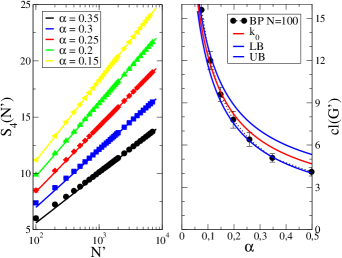
Figure 1: In the left panel, we report the entropy of cliques of size 4, as a function of the order $N^{\prime}$ for various values of $\alpha$. Symbols are BP results (each symbol averaged over 10 random graphs), full lines give the logarithm of the expected number of such cliques. On the right, we display the largest clique found by BP in graphs of size $N^{\prime}=100$, as a function of $\alpha$ (each symbol averaged over 10 random graphs). Results are consistent with theoretical bounds.

Results of this comparison are presented in Fig. 1. Finite size effects set in for small entropy values, which correspond to the logarithm of the maximum cliques number, while for larger $N^{\prime}$ the BP results perfectly coincide with the theoretical predictions. We note that in the case of cliques, and more in general for highly symmetric sub-graphs, it is possible to exploit symmetries to simplify the BP equations. The resulting equations have slightly different convergence properties compared to the generic BP ones. The largest cliques size found by our algorithm are in agreement with the (fairly tight) rigorous bounds also for small value of $N^{\prime}=100$, see right panel of Fig. 1. In the explicit constructions of cliques both the decimation and the reinforcement techniques have been used (the latter one being substantially faster).

Finding and couting small subgraphs is one of the major steps in the search for network motifs [17, 18, 19]. In contrast to exhaustive algorithms [17, 19], BP is able to handle the problem even for medium size subgraphs. Further more, working at finite temperature allows for non-perfect alignments, an thus for identifying, e.g., dense subgraphs instead of perfect cliques. A detailed exploration of this possibility goes beyond the scope of this letter.

Aligning sparse random graphs — In the second problem, we use BP to align two sparse random graphs $G$ and $G^{\prime}$ with identical numbers of nodes, $N=N^{\prime}$, and links, $M=M^{\prime}$. The injective mapping $\pi$ thus becomes a permutation. To study the best GA as a function of the inherent similarity between the two graphs, we construct $G$ and $G^{\prime}$ such that they have $M-M_{rand}$ links in common, the other $M_{rand}$ are chosen independently in the two graphs [20]. Note that for $M_{rand}=0$, the problem reduces to identify an isomorphism between the graphs. Due to the specific construction this isomorphism is trivially given by the identical permutation, $\pi_{i}=i$, but this information is neither known nor exploitable by the algorithm; it serves only for a simple evaluation of the simulation results. For $M_{rand}=M$, the two graphs are independent, and the number of alignable links is monotonously decreasing with $M_{rand}$.

Results for the alignment of $G$ and $G^{\prime}$ without node similarities ($c_{i,\pi_{i}}\equiv 0$) are given in the first panel of Fig. 2. For $M_{rand}=0$, BP always identifies correctly the isomorphism between the two graphs. In the other limiting case, $M_{rand}=M$ the number of aligned links is much smaller, and depends on the graph realization and the initial condition of the BP messages. In between the two extremes we find a transition in the algorithmic behavior at some $\bar{M}_{rand}$ where the identical permutation has the same value of $\cal H$ as the best alignment of two independent graphs. Above $\bar{M}_{rand}$, the number of aligned links is found to be almost constant, and equals the independent-graph case. For $0<M_{rand}<\bar{M}_{rand}$ the BP solutions fall into two different classes: one being close to the identical permutation with a high number of aligned links (green symbols in Fig. 2), and one having $\cal H$-values coherent with the alignment of two independent graphs (red symbols). The relative fraction of the first case is shown in the inset, it decreases when approaching $\bar{M}_{rand}$.

The behavior changes, when node similarities (cf. Eq. (1)) are used to bias BP toward the identical permutation. We set $c_{i,\pi_{i}}=c\delta_{i,\pi_{i}}$ for $i=1,...,K$, and $c_{i,\pi_{i}}=0$ for $i>K$, with $K\in\{0,...,N\}$. The parameter $K$ controls the number of biased nodes, and $c$ controls the strength of this bias. Interestingly, already a low value of $K$ is sufficient to let BP always find the lower energy solutions in the region $0<M_{rand}<\bar{M}_{rand}$. Results for different values of $K$ and $c$ are shown in the second panel of Fig 2. We observe that excessively high values of $K$ or $c$ decrease the performance of the algorithm for large $M_{rand}$ by forcing it towards solutions of less aligned links but more self-aligned nodes.

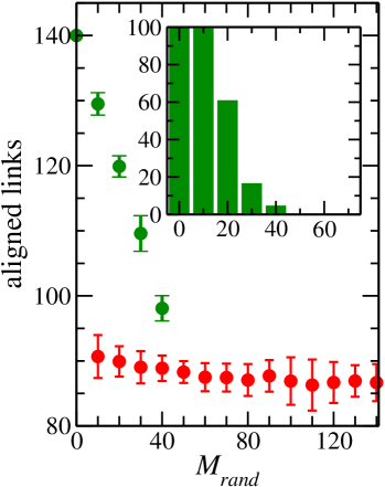
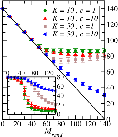
Figure 2: The number of aligned links as a function of the number $M_{rand}$ of independent links in $G$ and $G^{\prime}$, for $N=N^{\prime}=80$ and $M=M^{\prime}=140$ (each data point averaged over 30 random-graph pairs and 5 BP runs). First panel: Results for alignment without node similarities ($K=0$). For positive but not two large $M_{rand}$ the solutions fall into two classes: Green symbols represent close-to-identical permutations of high number of aligned links, red symbols represent results which are close to the alignment of two independent graphs. The inset shows the fraction of BP runs leading to a close-to-identical permutation. Second panel: Results for different values of the similarity parameters $K$ and $c$, the best performance is obtained for $K=10$ and $c=1$ (small bias). The inset shows the number of self-aligned nodes, it drops when the bias is not too large and $M_{rand}>\bar{M}_{rand}$.

Finding interacting protein partners from multi-species sequence data — Despite the fundamental importance of protein-protein interactions in most biological processes, identifying interaction partners is experimentally and computationally a major problem. As a proof-of-concept application for GA we consider two signaling proteins, namely a histidine sensor kinase (SK) and a response regulator (RR). Their interaction forms the central part of two-component signal transduction (TCS), which is the most prominent signal transduction mechanism in bacteria. Each bacterium contains ${\cal O}(10)$ interacting SK/RR pairs forming different TCS pathways; and the necessity to trigger the correct answer for each specific extracellular signal forbids crosstalk between pathways. So, even if all different SK in one species are homologous (and therefore structurally and functionally similar), and the same is true for all RR, only specific samples of these two protein families interact. Our question here is, if GA can help to identify interaction partners.

We start from a large collection of SK sequences extracted from hundreds of bacterial genomes, and a second large collection of RR sequences coming from the same bacteria, and we aim at extracting interacting SK/RR pairs, exploiting sequence similarities of proteins inside each family. The basic idea is simple: Two SK with very similar amino-acid sequences will (due to their probably recent common evolutionary origin) interact with two similar RR. Globally spoken, an alignment of two similarity networks - one for the SK family, one for the RR family - might be able to pair a large fraction of all those SK and RR which actually belong to common TCS pathways [12]. Our data set consists of two multiple-sequence alignments (with gaps) for 2546 SK and 2546 RR proteins from 231 genomes [21]. They are selected such that, due to the frequent coding of an entire TCS in one operon, the correct mapping is known, and can be used a posteriori to verify our GA results.

Similarity networks for each protein family are constructed as $k$NN graphs: Each protein is linked to the $k$ most similar proteins, where similarity is measured via the Hamming distance $d_{ij}$ between the aligned aminoacid sequences of two proteins $i$ and $j$. The link weight is given as $w_{ij}=\exp{[-{d^{2}_{ij}}/{d^{2}_{k}}]}$, with $d_{k}$ being the average distance between each protein and its $k$th neighbor. One might use more sophisticated distance measures (e.g. alignment scores), but due to the proof-of-concept character of this application we have chosen the simplest possible measure. To identify interaction partners, we must align only proteins inside the same species (formally implemented by $c_{i,i^{\prime}}=-\infty$ for all $i$ and $i^{\prime}$ belonging to different species). Finally, we have introduced various amounts of information about real interaction partners, by randomly introducing positive similarities between a number of actual interaction partners (training set). The results are summarized in the following table for different $k$ and training-set sizes. Error bars result from an average over different random training sets. The values display the fraction of correctly aligned protein pairs in between all proteins not being in the training set.

training set	3NN, $k=3$	6NN, $k=6$	9NN, $k=9$
2000	88.7 $\pm$ 1.7	89.8 $\pm$ 1.9	90.5 $\pm$ 1.7
1000	76.2 $\pm$ 1.3	78.7 $\pm$ 1.0	79.6 $\pm$ 0.8
500	67.4 $\pm$ 1.9	73.1 $\pm$ 1.4	75.0 $\pm$ 1.0
0	48.1	58.9	64.7

We note that even without training set, almost 65% of all proteins are correctly matched (for $k=9$). This number has to be compared to a random matching, where only $231/2546\sim 9\%$ correct matchings would be expected. The introduction of a training set improves strongly the performance, for a training set of 2000 protein pairs, about 90% of the remaining 546 proteins are correctly aligned. These results beautifully demonstrate that the original idea to exploit sequence similarity of proteins across species is actually providing information about who is interacting with whom.

Conclusion — In this letter we have presented a distributed (parallel) algorithm for graph-alignment problems. The new technique is based on the cavity method and allows to deal efficiently with optimization problems under (global) topological constraints. The results on famous problems such as sub-graph isomorphism and graph alignment on random graphs are in remarkable agreement with known rigorous bounds. Problems of this type are often encountered in the analysis of large-scale data in many fields of science, computational biology in first place.

References

- [1] D.J. Watts M. Newman, A.L. Barabasi. The Structure and Dynamics of Networks. Princeton University Press, Princeton, 2006.
- [2] J. Berg and M. Lässig. Proc. Natl. Acad. Sci., 103:10967, 2006.
- [3] Z. Li, S. Zhang, Y. Wang, X. Zhang, and L. Chen. Bioinformatics, 23:1631, 2007.
- [4] R. Singh, J. Xu, and B. Berger. Proc. Natl. Acad. Sci., 105:12763, 2008.
- [5] R. M. Karp. In R. E. Miller and J. W. Thatcher, editors, Complexity of Computer Computations, pages 85–103. New York: Plenum, 1972.
- [6] R Boppana and MM Halldorsson. BIT, 32(2):180–196, 1992.
- [7] B. B. Bollobas. Random graphs. Cambridge, University Press, 2001, 2nd ed. edition, 1985.
- [8] M. Mezard, G. Parisi, and R. Zecchina. Science, 297:812, 2002.
- [9] A. Braunstein, M. Mezard, and R. Zecchina. Random Structures and Algorithms, 27:201–226, 2005.
- [10] A. Montanari M. Mezard. Information, Physics, and Computation. Oxford University Press, Oxford, 2009.
- [11] M. Bayati, C. Borgs, A. Braunstein, J. Chayes, A. Ramezanpour, and R. Zecchina. Physical Review Letters, 101:037208, 2008.
- [12] A. K. Ramani and E. M. Marcotte. J. Mol. Biol., 327:273, 2003.
- [13] B.J. Frey and D. Dueck. Science, 315:972, 2007.
- [14] M. Leone, S. Sumedha, and M. Weigt. Bioinformatics, 23:2708, 2007.
- [15] M. Leone, Sumedha, and M. Weigt. Europ. Phys. J. B, 66:125, 2008.
- [16] A. Braunstein and R. Zecchina. Phys. Rev. Lett., 96:030201, 2006.
- [17] R. Milo, N. Kashtan, S. Itzkovitz, D. Chklovskii, and U. Alon. Science, 298:824, 2002.
- [18] J. Berg and M. Lässig. Proc. Natl. Acad. Sci., 101:14689, 2004.
- [19] F. Picard, J.J. Daudin, M. Koskas, S. Schbath, and S. Robin. J. Comp. Biol, 15(1):1, 2008.
- [20] M. Kolar, J. Berg, and M. Lässig. BMC Systems Biology, 2:90, 2008.
- [21] M. Weigt, R.A. White, H. Szurmant, J.A. Hoch, and T. Hwa. Proc. Natl. Acad. Sci., 106:67, 2009.