Entanglement induced transparency and applications

Abstract

We point out a symmetry exhibited by pairs of entangled states and discuss its possible applications in quantum information. More specifically, we consider quadripartite systems prepared in bipartite product states of the form $|\Psi\rangle=|\psi\rangle_{12}\otimes|\psi\rangle_{34}$ and let the uncorrelated subsystems $14$ and $23$ interact by a given unitary $U_{14}\otimes U_{23}$: we show that the entanglement between the noninteracting subsystems $12$ and $34$ may induce transparency, i.e. makes $|\Psi\rangle$ an eigenstate of the unitary. We investigate the occurrence of this phenomenon both in continuous variable and qubit systems, and discuss its possible applications to bath engineering, double swapping and remote inversion.

I Introduction

Entanglement is a relevant resource for quantum information processing and considerable efforts in this field have been devoted to investigate its generation, characterization, manipulation and storing eres ; edet ; eman . It is a general fact that the interaction with external systems may lead to entanglement degradation and, in turn, much attention has been payed to design and implement schemes suitable to preserve and restore entanglement BB1 ; BB2 . Among the other approaches, the analysis of symmetries is a powerful tool to investigate the separability problem and the dynamics of entanglement, as well as to individuate systems of interest for quantum information processing, as for example decoherence-free subspaces DFS97 and cluster states cl1 . In this paper we follow the above intuition and exploit a specific symmetry exhibited by pairs of entangled states for applications to bath engineering, double swapping and remote inversion.

The basic idea is to consider quadripartite systems prepared in bipartite product states of the form $|\Psi\rangle=|\psi\rangle_{12}\otimes|\psi\rangle_{34}$ and let the uncorrelated systems $14$ and $23$ interact by unitaries of the form $U_{14}\otimes U_{23}$. As we will see, there are conditions leading to entanglement induced transparency, namely conditions in which entanglement of the systems $12$ and $34$ preserve the initial state and its properties during the evolution. In other words, the overall state $|\Psi\rangle$ becomes an eigenstate of $U_{14}\otimes U_{23}$. In the following we investigate the occurrence of this phenomenon both in continuous variable and qubit systems, and discuss possible applications in quantum information processing.

The paper is structured as follows. In section II we describe entanglement induced transparency in continuous variable systems and investigate in details the peculiar role of twin beams, i.e maximally entangled states at fixed energy. We also give the phase-space analysis of the effect to discuss its robustness to pertubations and the evolution of entanglement of formation. In Section III we address application of entanglement induced transparency to bath engineering. In Section IV, we consider the discrete variable counterpart of entanglement induced transparency and describe its application to the remote inversion of an operation acting on two qubits belonging to two different entangled states. Section V closes the paper with some concluding remarks.

II Entanglement induced transparency in continuous variable systems

Let us first consider continuous variable systems to illustrate the effect of entanglement induced transparency (EntIT). In particular we show the crucial role played by twin-beam (TWB) entanglement. We address a system composed by four modes, with field operators $a_{k}$, $k=1,..,4$ and consider quadripartite (pure) state of the form

$$|\psi_{\rm in}\rangle=\sum_{n,m}\psi_{n,m}|n\rangle_{1}\otimes|m\rangle_{2}\otimes\sum_{h,k}\omega_{h,k}|h\rangle_{3}\otimes|k\rangle_{4}\>.$$ (1)

Then we make the modes 14 and 23 interact through bilinear Hamiltonians, as those describing the interaction of modes in a beam splitter. We denote by $U_{14}(\phi)$ and $U_{23}(\varphi)$ the corresponding unitary operations, which lead to the following Heisenberg evolution

$$U_{hk}^{{\dagger}}(\alpha)a_{k}U_{hk}(\alpha) =a_{h}\cos\alpha+a_{k}\sin\alpha$$ (2a)

$$U_{hk}^{{\dagger}}(\alpha)a_{h}U_{hk}(\alpha) =-a_{h}\sin\alpha+a_{k}\cos\alpha$$ (2b)

for the field modes. This corresponds to have beam splitters with transmissivities $T_{14}=\cos^{2}\phi$ and $T_{23}=\cos^{2}\varphi$. Upon expanding Fock number states $|n\rangle_{k}=(n!)^{-1/2}(a_{k}^{\dagger})^{n}|0\rangle$ and using mode transformation (2) one obtains:

$$|\psi_{\rm out}\rangle =U_{14}(\phi)\otimes U_{23}(\varphi)|\psi_{\rm in}\rangle$$ (3)

$$=\sum_{n,m,h,k}\frac{\psi_{n,m}\,\omega_{h,k}}{\sqrt{n!\,m!\,h!\,k!}}$$

$$\times \sum_{s=0}^{n}\sum_{t=0}^{m}\sum_{r=0}^{h}\sum_{u=0}^{k}(-1)^{r+u}{n\choose s}{m\choose t}{h\choose r}{k\choose u}$$

$$\times \sqrt{(n-s+u)!\,(m-t+r)!\,(h-r+t)!\,(k-u+s)!}$$

$$\times (\cos\phi)^{n+k-s-u}(\sin\phi)^{s+u}(\cos\varphi)^{m+h-t-r}(\sin\varphi)^{t+r}$$

$$\times |n-s+u\rangle_{1}|m-t+r\rangle_{2}|h-r+t\rangle_{3}|k-u+s\rangle_{4}$$ (4)

where, for the sake of simplicity, we omitted the tensor product symbol in the last line. The conditions for transparency $|\psi_{\rm out}\rangle=|\psi_{\rm in}\rangle$, can be obtained by imposing $\langle nmhk|\psi_{\rm in}\rangle=\langle nmhk|\psi_{\rm out}\rangle$ for all the basis elements $|nmhk\rangle\equiv|n\rangle_{1}|m\rangle_{2}|h\rangle_{3}|k\rangle_{4}$). It turns out that the whole set of equations is subsumed by a single condition

$$\psi_{1,1}\,\omega_{1,1}= \cos(2\phi)\cos(2\varphi)\psi_{1,1}\,\omega_{1,1}$$

$$+\frac{\cos(2\phi)\sin(2\varphi)}{\sqrt{2}}(\psi_{1,0}\,\omega_{2,1}-\psi_{1,2}\,\omega_{0,1})$$

$$+\frac{\sin(2\phi)\cos(2\varphi)}{\sqrt{2}}(\psi_{0,1}\,\omega_{1,2}-\psi_{2,1}\,\omega_{1,0})$$

$$+\frac{\sin(2\phi)\sin(2\varphi)}{2}$$

$$\times (\psi_{2,2}\,\omega_{0,0}-\psi_{0,2}\,\omega_{0,2}-\psi_{2,0}\,\omega_{2,0}+\psi_{0,0}\,\omega_{2,2}).$$ (5)

If $\psi_{n,m}$ and $\omega_{h,k}$ are generic, then the only solution of (5) is $\phi=\varphi=0$, i.e., the BSs transmissivity should be equal to 1 (trivial solution). For completeness, we note that also $\phi=\varphi=\pi/2$ is a solution, but, in this case, the two mode are just exchanged. In particular, these results can be applied to separable states, in which $\psi_{n,m}$ and $\omega_{h,k}$ can be written as product of two terms respectively. In other words, classical correlations are not enough to obtain the transparency.

Let us now consider the case of photon-number entangled states, namely states with $\psi_{n,m}\propto\delta_{nm}\,\psi_{n}$ and $\omega_{h,k}=\delta_{kh}\,\psi_{k}$, $\delta_{nm}$ being the Kronecker delta. TWBs belong to this class, as well as the so-called pair-coherent states aga86 ; aga05 , which find applications in quantum communication us1 ; us2 . In this case Eq. (5) reduces to:

$$\psi_{1}\,\omega_{1}= \cos(2\phi)\cos(2\varphi)\,\psi_{1}\,\omega_{1}$$

$$+2\cos(\phi)\sin(\phi)\cos(\varphi)\sin(\varphi)$$

$$\times(\psi_{2}\,\omega_{0}+\psi_{0}\,\omega_{2})\>,$$ (6)

which, in general, admits only the trivial solution $\phi=\varphi=0$. However, if one choose $\psi_{n}=\omega_{n}=\lambda^{n}$, corresponding to a pair of TWB states, Eq. (6) simplifies to $\cos[2(\phi-\varphi)]=1$ i.e., one has the transparency effect by choosing $\phi=\varphi$. We can conclude that only TWB states may give rise to the EntIT due to their peculiar analytical expression and, in turn, the transparency is induced by the TWB entanglement. It is worth to note that when EntIT occurs, then the quadripartite input state is an eigenstate of the unitary transformation $U_{14}(\phi)\otimes U_{23}(\phi)$. Notice that EntIT takes place for any value of the beam splitters transmissivity provided they are equal.

In the following, we focus the attention on the case of a pair of TWB, $|r\rangle\rangle$ and $|s\rangle\rangle$ for modes 12 and 34 and mix modes 14 and 23 of state in two balanced BSs (Fig. 1). The initial state $|\psi_{\rm in}\rangle$ is given by two TWB states with (real) parameters $r$ and $s$, namely:

$$|\psi_{\rm in}\rangle=S_{12}(r)\otimes S_{34}(s)|0\rangle=|r\rangle\rangle\otimes|s\rangle\rangle,$$ (7)

where $S_{hk}(\zeta)=\exp(\zeta a_{h}^{{\dagger}}a_{k}^{{\dagger}}-h.c.)$ is the two-mode squeezing operator acting onto modes $h$ and $k$, respectively, and $a_{l}$ is the annihilation operator of mode $l$.

Figure 1: Entanglement induced transparency/swapping when the pair of TWB, $|r\rangle\rangle$ and $|s\rangle\rangle$, are mixed at two balanced beam splitters.

Thanks to the transformations (2), the state emerging from the BSs can be written as:

$$|\psi_{\rm out}\rangle= U_{14}\otimes U_{23}|\psi_{\rm in}\rangle$$ (8)

$$= \exp\Bigg{\{}\frac{1}{2}\Big{[}(r+s)(a_{1}^{{\dagger}}a_{2}^{{\dagger}}+a_{3}^{{\dagger}}a_{4}^{{\dagger}})$$

$$+(r-s)(a_{1}^{{\dagger}}a_{3}^{{\dagger}}+a_{2}^{{\dagger}}a_{4}^{{\dagger}})-h.c.\Big{]}\Bigg{\}}|0\rangle.$$ (9)

Form Eq. (9) we see that:

$$\mbox{if }s=r\quad \Rightarrow\quad |\psi_{\rm out}\rangle=|\psi_{\rm in}\rangle;$$ (10)

$$\mbox{if }s=-r\quad \Rightarrow\quad |\psi_{\rm out}\rangle=S_{13}(r)S_{24}(r)|0\rangle.$$ (11)

In other words, in the case (10) we have the EntIT effect, i.e., $|\psi_{\rm in}\rangle\to|\psi_{\rm in}\rangle$; in the case (11) we obtain $S_{12}(r)\otimes S_{34}(r)|0\rangle\to S_{13}(r)\otimes S_{24}(r)|0\rangle$, i.e., entanglement is “swapped” from mode 12 and 34 to modes 13 and 24 (note that modes 1 and 3, as well as modes 2 and 4, did not directly interact each other). In the last case no measurement is required to obtain (double) entanglement swapping, even if to this aim one should have two identical states as inputs (double swapping). More generally, if the BSs have transmissivity $T_{14}=\cos^{2}\phi$ and $T_{23}=\cos^{2}\varphi$, then the outgoing state reads:

$$|\psi_{\rm out}\rangle= \exp\big{[}(r\cos\phi\cos\varphi+s\sin\phi\sin\varphi)a_{1}^{{\dagger}}a_{2}^{{\dagger}}$$

$$+(r\sin\phi\sin\varphi+s\cos\phi\cos\varphi)a_{3}^{{\dagger}}a_{4}^{{\dagger}}$$

$$+(r\cos\phi\sin\varphi-s\sin\phi\cos\varphi)a_{1}^{{\dagger}}a_{3}^{{\dagger}}$$

$$+(r\sin\phi\cos\varphi-s\cos\phi\sin\varphi)a_{2}^{{\dagger}}a_{4}^{{\dagger}}-h.c.\big{]}|0\rangle,$$ (12)

which reduces to (9) if $\phi=\varphi=\pi/4$. Investigating Eq. (12), we see that if $\varphi=\phi$ we have:

$$|\psi_{\rm out}\rangle= \exp\big{[}(r\cos^{2}\phi+s\sin^{2}\phi)a_{1}^{{\dagger}}a_{2}^{{\dagger}}$$

$$+(r\sin^{2}\phi+s\cos^{2}\phi)a_{3}^{{\dagger}}a_{4}^{{\dagger}}$$

$$+(r-s)\cos\phi\sin\phi(a_{1}^{{\dagger}}a_{3}^{{\dagger}}+a_{2}^{{\dagger}}a_{4}^{{\dagger}})-h.c.\big{]}|0\rangle,$$ (13)

and one can always obtain the EntIT for $r=s$, whereas there is no way to obtain perfect swapping.

II.1 Phase-space analysis and robustness of EnIT

In this section we characterize the state (13) in the phase-space in order to address the distribution of two-mode entanglement among all the possible partitions and the robustness of the EntIT effect. In order to simplify the formalism, we will use the following notation for the input/output modes $h,k,\ldots$: when we write “$\square_{hk\ldots}$”, we refer to input modes, whereas writing “$\square^{(hk\ldots)}$” output modes are considered. Since the involved states are Gaussian and the evolution preserves this character, in order to characterize the output states we consider the evolution of the covariance matrix (CM) gsb . The CM associated with the two-mode squeezed vacuum state $|\psi_{hk}(r)\rangle\rangle=S_{hk}(r)|0\rangle$ of modes $h$ and $k$ reads:

$${\boldsymbol{\Sigma}}_{hk}(r)=\frac{1}{2}\left(\begin{array}[]{c|c}\cosh 2r\,{\mathbbm{1}}_{2}&\sinh 2r\,{\boldsymbol{\sigma}}_{3}\\ \hline\cr-\sinh 2r\,{\boldsymbol{\sigma}}_{3}&\cosh 2r\,{\mathbbm{1}}_{2}\end{array}\right),$$ (14)

where ${\mathbbm{1}}_{2}$ is the $2\times 2$ identity matrix and ${\boldsymbol{\sigma}}_{3}=\mbox{Diag}(1,-1)$ is the Pauli matrix. Thus, the four-mode covariance matrix of state (7) is given by:

$${\boldsymbol{\Sigma}}_{1234}={\boldsymbol{\Sigma}}_{12}(r)\oplus{\boldsymbol{\Sigma}}_{34}(s)=\left(\begin{array}[]{c|c}{\boldsymbol{\Sigma}}_{12}(r)&{\boldsymbol{0}}\\ \hline\cr{\boldsymbol{0}}&{\boldsymbol{\Sigma}}_{34}(s)\end{array}\right).$$ (15)

The CM after the evolution through the BSs can be obtained as follows:

$${\boldsymbol{\Sigma}}^{(1234)}(\phi,\varphi)={\boldsymbol{S}}^{T}(\phi,\varphi){\boldsymbol{\Sigma}}_{1234}{\boldsymbol{S}}(\phi,\varphi)$$ (16)

where:

$${\boldsymbol{S}}(\phi,\varphi)=\left(\begin{array}[]{c|c|c|c}\cos\phi\,{\mathbbm{1}}_{2}&{\boldsymbol{0}}&{\boldsymbol{0}}&\sin\phi\,{\mathbbm{1}}_{2}\\ \hline\cr{\boldsymbol{0}}&\cos\varphi\,{\mathbbm{1}}_{2}&\sin\varphi\,{\mathbbm{1}}_{2}&{\boldsymbol{0}}\\ \hline\cr{\boldsymbol{0}}&-\sin\varphi\,{\mathbbm{1}}_{2}&\cos\varphi\,{\mathbbm{1}}_{2}&{\boldsymbol{0}}\\ \hline\cr-\sin\phi\,{\mathbbm{1}}_{2}&{\boldsymbol{0}}&{\boldsymbol{0}}&\cos\phi\,{\mathbbm{1}}_{2}\\ \end{array}\right),$$ (21)

is the symplectic transformation associated with mode transformation (2). Now, if we use the following $2\times 2$ block matrix decomposition of a $8\times 8$ matrix:

$${\boldsymbol{A}}=\left(\begin{array}[]{c|c|c|c}{\boldsymbol{A}}_{11}&{\boldsymbol{A}}_{12}&{\boldsymbol{A}}_{13}&{\boldsymbol{A}}_{14}\\ \hline\cr{\boldsymbol{A}}_{21}&{\boldsymbol{A}}_{22}&{\boldsymbol{A}}_{23}&{\boldsymbol{A}}_{24}\\ \hline\cr{\boldsymbol{A}}_{31}&{\boldsymbol{A}}_{32}&{\boldsymbol{A}}_{33}&{\boldsymbol{A}}_{34}\\ \hline\cr{\boldsymbol{A}}_{41}&{\boldsymbol{A}}_{42}&{\boldsymbol{A}}_{43}&{\boldsymbol{A}}_{44}\end{array}\right),$$ (22)

and introduce the notation:

$$[[{\boldsymbol{A}}]]_{hk}\equiv\left(\begin{array}[]{c|c}{\boldsymbol{A}}_{hh}&{\boldsymbol{A}}_{hk}\\ \hline\cr{\boldsymbol{A}}_{kh}&{\boldsymbol{A}}_{kk}\\ \end{array}\right),$$ (23)

then the CM ${\boldsymbol{\Sigma}^{(hk)}}$ associated with the reduced state $\varrho^{(hk)}=\mbox{Tr}_{n,m}[\varrho^{(1234)}]$, with $n\neq m\neq h\neq k$, $\varrho_{1234}$ being the density matrix of the state (12):

$${\boldsymbol{\Sigma}^{(hk)}}=[[{\boldsymbol{\Sigma}^{(1234)}}]]_{hk}.$$ (24)

Starting from ${\boldsymbol{\Sigma}^{(hk)}}$ one can easily evaluate the purity, the separability and the entanglement of formation of the reduced states $\varrho^{(hk)}$. As an example, we plot in Fig. 2 the minimum symplectic eigenvalue $\tilde{\kappa}_{-}$ of the partially transposed of the reduced density matrices $\varrho^{(12)}$, $\varrho^{(13)}$ as a function of $x\in[-1,1]$, where we fixed $r$ and put $x=s/r$. For the reduced density matrices $\varrho^{(34)}$ and $\varrho^{(24)}$ one has the same results. Recalling that a bipartite Gaussian state is separable iff $\tilde{\kappa}_{-}\geq 1/2$, from Fig. 2 we can see the swapping of entanglement; notice that there is an interval of values of $x$ for which all the four partitions are not separable.

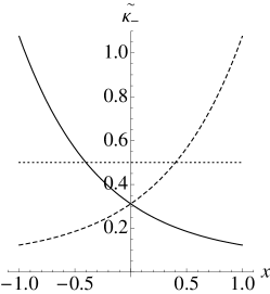
Figure 2: Plot of the minimum symplectic eigenvalue $\tilde{\kappa}_{-}$ of (partially transposed) density matrices $\varrho^{(12)}$ (solid line) and $\varrho^{(13)}$ (dashed) as functions of $x=s/r$. We chose two balanced BSs, i.e., $\phi=\varphi=\pi/4$, and put $r=0.7$. See the text for details. The dotted line refers to the separability threshold $\tilde{\kappa}_{-}=1/2$: if $\tilde{\kappa}_{-}\geq 1/2$ the state is separable.

In the present case, due to the symmetry of the reduced states, their entanglement of formation is given by EOFM

$$E_{f}=\left(\chi+\frac{1}{2}\right)\ln\left(\chi+\frac{1}{2}\right)-\left(\chi-\frac{1}{2}\right)\ln\left(\chi-\frac{1}{2}\right),$$ (25)

where $\chi=(\tilde{\kappa}_{-}^{2}+1/4)/(2\tilde{\kappa}_{-})$. We have seen that EntIT is achieved requiring $s=r$ and $\varphi=\phi$. In order to evaluate the robustness of the effect, we address the fidelity between $\varrho_{12}$ and $\varrho^{(12)}$, the input and the output state of modes 1 and 2, respectively. Since they are both Gaussian states, the fidelity is given by:

$$F=\left\{\hbox{Det}\left[\boldsymbol{\Sigma}_{12}+\boldsymbol{\Sigma}^{(12)}\right]\right\}^{-1/2}.$$ (26)

The analytic expression of $F$ is quite cumbersome; however, we report two relevant series expansions with respect to the TWB parameters ($r$ and $s$) and the BSs transmissivities ($T_{14}=\cos^{2}\phi$ and $T_{23}=\cos^{2}\varphi$). The first expansion concerns the TWB parameters in the case $\varphi=\phi$ and reads:

$$F\approx 1-\frac{1}{2}\left[3+\sin^{2}\phi\,\cos(2\phi)\right](s-r)^{2};$$ (27)

the second one addresses the BSs transmissivities:

$$F\approx f+f^{2}\,\sin(2\phi)\,\cos^{2}(\phi)\,\sinh^{2}(r-s)\,(\phi-\varphi),$$ (28)

where $f\equiv f(r,s,\phi)$ is given by:

$$f=\frac{1}{1+[1+\cos^{2}(\phi)]\sin^{2}(\phi)\sinh^{2}(r-s)}.$$ (29)

Eq. (27) shows the robustness of the effect with respect to fluctuations of $s$, whereas, from Eq. (28), we conclude that the fluctuations of BSs transmissivities may be quite relevant.

III Application to bath engineering

It is well known that correlated noise may enhance the capacity of a quantum channel CM02 ; KB04 . Moreover, in the last years the bosonic quantum channels with memory have attracted a growing interest DK05 ; NJC05 ; CL09 . These channels are characterized by Gaussian distributed-thermal noise and correlations between the environmental modes. Even if only classical correlations have been addressed so far, it has been demonstrated that uncorrelated phase-sensitive environments, i.e, uncorrelated noisy channels with squeezed fluctuations can been addressed for preservation of macroscopic quantum coherence TABK88 ; PT94 ; NL98 or for improving teleportation of squeezed states SO03 . A new insight to the properties of this kind of channels, when also nonclassical correlations are present, may be given by applying our analysis to a simple case of bath engineering, where entangled bath oscillators let properties such as entanglement and purity of an input state survive longer than uncorrelated ones do.

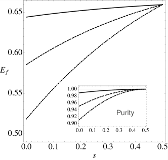
Figure 3: Entanglement of formation, $E_{f}$, of the state $\varrho^{(12)}$ a function of the TWB parameter $s$ used to engineer the coupling (see Fig. 1) for $r=0.5$ and different values of loss parameter $\Gamma$, from top to bottom: $\Gamma=0.01$ (solid), $0.05$ (dashed) and $0.1$ (dot-dashed). The inset shows the corresponding value of the purity as a function of $s$.

Let us now assume that the BSs in Fig. 1 describe linear losses (with the vacuum as input for both the ports 3 and 4, i.e., $s=0$). In this case, it is useful to define $\phi=\arccos\sqrt{1-\Gamma}$, where $T=\cos^{2}\phi$ is the BS transmissivity (we assume that both the BS have the same transmissivity, i.e., $\varphi=\phi$): if $\Gamma=0$ there aren’t losses, is $\Gamma=1$ the state is completely lost. We will refer to $\Gamma$ as loss parameter. As a matter of fact, losses degrade the properties of the outgoing state $\varrho^{(12)}$ of mode 1 and 2; however, we can use the results of the previous section to engineer the state $\varrho_{34}$ to recover the degraded state (see Fig. 1). If $\varrho_{12}$ is initially in a TWB state with TWB parameter $r$, then, by choosing as $\varrho_{34}$ a TWB with parameter $s=r$ (EntIT configuration), we have $\varrho^{(12)}=\varrho_{12}$: the state is totally recovered. Nevertheless, a partial recover is achieved also when $s<r$ (of course, if $s>r$ the outgoing state $\varrho^{(12)}$ has properties more related to $\varrho_{34}$ than to $\varrho_{12}$). This is shown in Fig. 3, where we plot the $E_{f}$ and the purity $\mu=\{(16\hbox{Det}[{\boldsymbol{\Sigma}^{(12)}}]\}^{-1/2}$ of $\varrho^{(12)}$ as functions of $s$ and different values of the other involved parameters.

IV Two two-qubit systems invariance via “remote inversion”

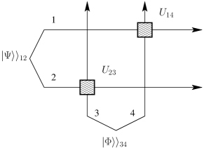
Figure 4: Qubits 14 and 23 of two two-qubit states undergo the unitary evolutions $U_{14}$ and $U_{23}$, respectively.

Let us now consider the qubit couterpart of the continuous variable setup investigated above. In this scenario, sketched in Fig. 4, the qubits 14 and 23 of two two-qubit states $|\Psi\rangle\rangle_{12}$ and $|\Phi\rangle\rangle_{34}$ undergo the generic unitary evolutions $U_{14}$ and $U_{23}$, respectively, where:

$$U_{14}({\boldsymbol{\theta}})= \exp\left(-i\sum_{k=0}^{3}\theta_{k}\,\boldsymbol{\sigma}_{k}\otimes\boldsymbol{\sigma}_{0}\otimes\boldsymbol{\sigma}_{0}\otimes\boldsymbol{\sigma}_{k}\right),$$ (30)

$$= \,G_{0}({\boldsymbol{\theta}})\,\boldsymbol{\sigma}_{0}\otimes\boldsymbol{\sigma}_{0}\otimes\boldsymbol{\sigma}_{0}\otimes\boldsymbol{\sigma}_{0}$$

$$-\sum_{k=1}^{3}G_{k}({\boldsymbol{\theta}})\,\boldsymbol{\sigma}_{k}\otimes\boldsymbol{\sigma}_{0}\otimes\boldsymbol{\sigma}_{0}\otimes\boldsymbol{\sigma}_{k},$$ (31)

$$U_{23}({\boldsymbol{\phi}})= \exp\left(-i\sum_{k=0}^{3}\phi_{k}\,\boldsymbol{\sigma}_{0}\otimes\boldsymbol{\sigma}_{k}\otimes\boldsymbol{\sigma}_{k}\otimes\boldsymbol{\sigma}_{0}\right)$$ (32)

$$= \,G_{0}({\boldsymbol{\phi}})\,\boldsymbol{\sigma}_{0}\otimes\boldsymbol{\sigma}_{0}\otimes\boldsymbol{\sigma}_{0}\otimes\boldsymbol{\sigma}_{0}$$

$$-\sum_{k=1}^{3}G_{k}({\boldsymbol{\phi}})\,\boldsymbol{\sigma}_{0}\otimes\boldsymbol{\sigma}_{k}\otimes\boldsymbol{\sigma}_{k}\otimes\boldsymbol{\sigma}_{0},,$$ (33)

with ${\boldsymbol{\theta}}=(\theta_{0},\theta_{1},\theta_{2},\theta_{3})$, ${\boldsymbol{\phi}}=(\phi_{0},\phi_{1},\phi_{2},\phi_{3})$, $\boldsymbol{\sigma}_{k}$, $k=0,1,2,3$, are the Pauli matrices, $\boldsymbol{\sigma}_{0}={\mathbbm{1}}$, and:

$$G_{k}({\boldsymbol{x}})= \,e^{-i(x_{0}-x_{1}-x_{2}-x_{3})}\,$$

$$\times\left[1+\frac{1}{2}\sum_{n,m=1}^{3}g_{k}(n,m)\,e^{2i(x_{n}+x_{m})}\right],$$ (34)

${\boldsymbol{x}}=(x_{0},x_{1},x_{2},x_{3})$, with:

$$g_{k}(n,m)=\left\{\begin{array}[]{ll}+1&\mbox{if }k\neq n,m\\ 0&\mbox{if }n=m\\ -1&\mbox{elsewhere}\end{array}\right..$$ (35)

We are interested in finding the conditions on ${\boldsymbol{\theta}}$ and ${\boldsymbol{\phi}}$, that leave the input states unchanged. We restrict our analysis assuming that $|\Psi\rangle\rangle_{12}$ and $|\Phi\rangle\rangle_{34}$ are initially in the same state. Let us now consider as input states $|\Psi\rangle\rangle_{12}=\frac{1}{\sqrt{2}}\left(|00\rangle_{12}+|11\rangle_{12}\right)$ and $|\Phi\rangle\rangle_{34}=\frac{1}{\sqrt{2}}\left(|00\rangle_{34}+|11\rangle_{34}\right)$, where $|xy\rangle_{kh}=|x\rangle_{k}\otimes|y\rangle_{h}$. The four qubit initial state is then given by:

$$|\psi\rangle_{1234} =|\Psi\rangle\rangle_{12}\otimes|\Phi\rangle\rangle_{34}$$ (36)

$$=\frac{1}{2}\Big{(}|00\rangle_{14}|00\rangle_{23}+|01\rangle_{14}|01\rangle_{23}$$

$$\hskip 14.22636pt+|10\rangle_{14}|10\rangle_{23}+|11\rangle_{14}|11\rangle_{23}\Big{)}$$ (37)

$$=\frac{1}{2}\Big{(}\left|\left.\mbox{$\frac{\boldsymbol{\sigma}_{0}}{\sqrt{2}}$}\right\rangle\!\!\right\rangle_{14}\left|\left.\mbox{$\frac{\boldsymbol{\sigma}_{0}}{\sqrt{2}}$}\right\rangle\!\!\right\rangle_{23}+\left|\left.\mbox{$\frac{\boldsymbol{\sigma}_{1}}{\sqrt{2}}$}\right\rangle\!\!\right\rangle_{14}\left|\left.\mbox{$\frac{\boldsymbol{\sigma}_{1}}{\sqrt{2}}$}\right\rangle\!\!\right\rangle_{23}$$

$$\hskip 14.22636pt+\left|\left.\mbox{$i\frac{\boldsymbol{\sigma}_{2}}{\sqrt{2}}$}\right\rangle\!\!\right\rangle_{14}\left|\left.\mbox{$i\frac{\boldsymbol{\sigma}_{2}}{\sqrt{2}}$}\right\rangle\!\!\right\rangle_{23}+\left|\left.\mbox{$\frac{\boldsymbol{\sigma}_{3}}{\sqrt{2}}$}\right\rangle\!\!\right\rangle_{14}\left|\left.\mbox{$\frac{\boldsymbol{\sigma}_{3}}{\sqrt{2}}$}\right\rangle\!\!\right\rangle_{23}\Big{)}$$ (38)

where we re-arranged the tensor product elements in order to put in evidence the bipartite couples (14 and 23, respectively) involved by the transformations; from (37) to (38), we used the matrix notation for bipartite states LoPresti:00 . Now, after some algebra based on the properties of the Pauli matrices, one can easily find the following relations:

$$U({\boldsymbol{\theta}},{\boldsymbol{\phi}})\left|\left.\mbox{$\frac{\boldsymbol{\sigma}_{0}}{\sqrt{2}}$}\right\rangle\!\!\right\rangle_{14}\left|\left.\mbox{$\frac{\boldsymbol{\sigma}_{0}}{\sqrt{2}}$}\right\rangle\!\!\right\rangle_{23}=$$

$$\left[G_{0}({\boldsymbol{\theta}})-G_{1}({\boldsymbol{\theta}})+G_{2}({\boldsymbol{\theta}})-G_{3}({\boldsymbol{\theta}})\right]$$ (39a)

$$\times\left[G_{0}({\boldsymbol{\phi}})-G_{1}({\boldsymbol{\phi}})+G_{2}({\boldsymbol{\phi}})-G_{3}({\boldsymbol{\phi}})\right]\left|\left.\mbox{$\frac{\boldsymbol{\sigma}_{0}}{\sqrt{2}}$}\right\rangle\!\!\right\rangle_{14}\left|\left.\mbox{$\frac{\boldsymbol{\sigma}_{0}}{\sqrt{2}}$}\right\rangle\!\!\right\rangle_{23}$$

$$U({\boldsymbol{\theta}},{\boldsymbol{\phi}})\left|\left.\mbox{$\frac{\boldsymbol{\sigma}_{1}}{\sqrt{2}}$}\right\rangle\!\!\right\rangle_{14}\left|\left.\mbox{$\frac{\boldsymbol{\sigma}_{1}}{\sqrt{2}}$}\right\rangle\!\!\right\rangle_{23}=$$

$$\left[G_{0}({\boldsymbol{\theta}})-G_{1}({\boldsymbol{\theta}})-G_{2}({\boldsymbol{\theta}})+G_{3}({\boldsymbol{\theta}})\right]$$ (39b)

$$\times\left[G_{0}({\boldsymbol{\phi}})-G_{1}({\boldsymbol{\phi}})-G_{2}({\boldsymbol{\phi}})+G_{3}({\boldsymbol{\phi}})\right]\left|\left.\mbox{$\frac{\boldsymbol{\sigma}_{1}}{\sqrt{2}}$}\right\rangle\!\!\right\rangle_{14}\left|\left.\mbox{$\frac{\boldsymbol{\sigma}_{1}}{\sqrt{2}}$}\right\rangle\!\!\right\rangle_{23}$$

$$U({\boldsymbol{\theta}},{\boldsymbol{\phi}})\left|\left.\mbox{$i\frac{\boldsymbol{\sigma}_{2}}{\sqrt{2}}$}\right\rangle\!\!\right\rangle_{14}\left|\left.\mbox{$i\frac{\boldsymbol{\sigma}_{0}}{\sqrt{2}}$}\right\rangle\!\!\right\rangle_{23}=$$

$$\left[G_{0}({\boldsymbol{\theta}})+G_{1}({\boldsymbol{\theta}})+G_{2}({\boldsymbol{\theta}})+G_{3}({\boldsymbol{\theta}})\right]$$ (39c)

$$\times\left[G_{0}({\boldsymbol{\phi}})+G_{1}({\boldsymbol{\phi}})+G_{2}({\boldsymbol{\phi}})+G_{3}({\boldsymbol{\phi}})\right]\left|\left.\mbox{$i\frac{\boldsymbol{\sigma}_{2}}{\sqrt{2}}$}\right\rangle\!\!\right\rangle_{14}\left|\left.\mbox{$i\frac{\boldsymbol{\sigma}_{2}}{\sqrt{2}}$}\right\rangle\!\!\right\rangle_{23}$$

$$U({\boldsymbol{\theta}},{\boldsymbol{\phi}})\left|\left.\mbox{$\frac{\boldsymbol{\sigma}_{3}}{\sqrt{2}}$}\right\rangle\!\!\right\rangle_{14}\left|\left.\mbox{$\frac{\boldsymbol{\sigma}_{3}}{\sqrt{2}}$}\right\rangle\!\!\right\rangle_{23}=$$

$$\left[G_{0}({\boldsymbol{\theta}})+G_{1}({\boldsymbol{\theta}})-G_{2}({\boldsymbol{\theta}})-G_{3}({\boldsymbol{\theta}})\right]$$ (39d)

$$\times\left[G_{0}({\boldsymbol{\phi}})+G_{1}({\boldsymbol{\phi}})-G_{2}({\boldsymbol{\phi}})-G_{3}({\boldsymbol{\phi}})\right]\left|\left.\mbox{$\frac{\boldsymbol{\sigma}_{3}}{\sqrt{2}}$}\right\rangle\!\!\right\rangle_{14}\left|\left.\mbox{$\frac{\boldsymbol{\sigma}_{3}}{\sqrt{2}}$}\right\rangle\!\!\right\rangle_{23}$$

where we defined $U({\boldsymbol{\theta}},{\boldsymbol{\phi}})\equiv U_{14}({\boldsymbol{\theta}})U_{23}({\boldsymbol{\phi}})$ and used the property $A\otimes B|C\rangle\rangle=|ACB^{T}\rangle\rangle$ of the matrix representation of bipartite states. Hence, the input states are left unchanged if the condition ${\boldsymbol{\phi}}=-{\boldsymbol{\theta}}$ is met: in this case all the numerical coefficients appearing at the right hand sides of Eq.s (39) are equal to 1. The same result holds if we consider as input states $|\Psi\rangle\rangle_{12}$ and $|\Phi\rangle\rangle_{34}$ one of the three left Bell states. For a generic two qubit state the previous condition is not enough to leave it unchanged, and more condition on ${\boldsymbol{\theta}}$ are required (see Appendix A for a complete zoology).

We can also look at the invariance obtained for Bell states as follows. The action of an unitary transformation, acting on two qubits belonging to different couples of qubits initially in the same Bell state, can be canceled out by applying the inverse transformation to the remaining couple of qubits (choosing ${\boldsymbol{\phi}}=-{\boldsymbol{\theta}}$ formally corresponds to the inverse of the first transformation, of course, acting on a different system). For this effect (invariance), Bell states plays a crucial role: if we consider as starting states other than Bell states, the inversion of the operation is not enough to achieve the invariance, further conditions are needed, i.e., differently form the Bell state case, not all the classes of unitaries leads to invariance up to “remote inversion”.

V Conclusions

In this paper we have investigated in some details a useful symmetry exhibited by pairs of entangled states, which induces operation transparency, i.e the preservation of the state under the action of specific class of unitaries.

In continuous variable systems entanglement induced transparency occurs when two TWBs with the same energy are left unchanged after the evolution through two equal beam splitters. We have shown that entanglement is crucial for the effect and we have studied its occurrence and robustness. Besides, we have shown how EntIT may be useful to engineer baths with nonclassical correlations in order to preserve transmission of entanglement and the purity of TWBs during the propagation. Related to the EntIT effect is the double swapping: now entanglement is swapped between the modes of TWBs by simply changing the phase of the initial bipartite states before the interaction at two balanced BSs and without any measurement.

The investigation of the discrete-variable counterpart of the EntIt has brought us to the “remote inversion” effect, i.e., the action of an unitary transformation, acting on two qubits belonging to different couples of qubits initially in the same Bell state, can be canceled out by applying the inverse transformation to the remaining couple of qubits. This effect my be used to remotely control quantum operations over a quantum network.

Appendix A Zoology for qubit invariance via “remote inversion”

Here we assume that both the states $|\Psi\rangle\rangle_{12}$ and $|\Phi\rangle\rangle_{34}$ are equal to the same state:

$$|\psi\rangle\rangle=\sum_{h,k=0,1}a_{hk}|hk\rangle,$$ (40)

with $\sum_{h,k}a_{hk}^{2}=1$ (without loss of generality we choose only real coefficients). We have seen in Section IV that if $|\psi\rangle\rangle$ is one of the four Bell states, then the invariance is achieved for ${\boldsymbol{\phi}}=-{\boldsymbol{\theta}}$. In all the other cases the following further conditions are needed (of course, together with ${\boldsymbol{\phi}}=-{\boldsymbol{\theta}}$).

• $a_{00}=1$ or $a_{11}=1$ $\Rightarrow$ $\theta_{1}=\theta_{2}$.

• $a_{01}=1$ or $a_{10}=1$ $\Rightarrow$ $\theta_{1}=-\theta_{2}$.

• $a_{00},a_{11}\neq 0$, $a_{00}\neq a_{11}$, and $a_{01},a_{10}=0$ $\Rightarrow$ $\theta_{1}=\theta_{2}$.

• $a_{01},a_{10}\neq 0$, $a_{01}\neq a_{10}$, and $a_{00},a_{11}=0$ $\Rightarrow$ $\theta_{1}=-\theta_{2}$.

• $a_{hk}\neq 0,\forall h,k$:

  • $a_{00}=a_{11}$ and $a_{01}=a_{10}$ $\Rightarrow$ $\theta_{2}=\theta_{3}$.

  • $a_{00}=-a_{11}$ and $a_{01}=-a_{10}$ $\Rightarrow$ $\theta_{2}=-\theta_{3}$.

  • $a_{00}=-a_{11}$ and $a_{01}=a_{10}$ $\Rightarrow$ $\theta_{1}=\theta_{3}$.

  • $a_{00}=a_{11}$ and $a_{01}=-a_{10}$ $\Rightarrow$ $\theta_{1}=-\theta_{3}$.

• In all the other cases one should put ${\boldsymbol{\phi}}={\boldsymbol{\theta}}=0$, i.e., the states are left unchanged only if no operation is performed.

References

- (1) W. K. Wootters, Phil. Trans. R. Soc. Lond. A 356, 1717 (1998).
- (2) O. Guhne, G. Toth, Physics Reports 474, 1 (2009).
- (3) J. M. Raimond, M. Brune, S. Haroche, Rev. Mod. Phys. 73, 565 (2001).
- (4) D. Vitali and P. Tombesi, Phys Rev A 59, 4178 (1999).
- (5) S. Damodarakurup, et a., arXiv:0811.2654v1 [quant-ph].
- (6) P. Zanardi and M. Rasetti, Mod. Phys. Lett. B 11, 1085 (1997); P. Zanardi and M. Rasetti, Phys. Rev. Lett. 79, 3306 (1997).
- (7) H. J. Briegel and R. Raussendorf, Phys. Rev. Lett. 86, 910 (2001).
- (8) G. S. Agarwal, Phys. Rev. Lett. 57, 827 (1986).
- (9) G. S. Agarwal and A. Biswas, J. Opt B 7, 350 (2005).
- (10) V. C. Usenko, B. I. Lev, Phys. Lett. A 348, 17 (2005).
- (11) V. C. Usenko, M. G. A. Paris, Phys. Rev. A 75, 043812 (2007).
- (12) J. Eisert et al., Int. J. Quant. Inf. 1, 479 (2003); A. Ferraro et al., Gaussian States in Quantum Information, (Bibliopolis, Napoli, 2005); G. Adesso et al., J. Phys. A 40, 7821 (2007); S. L. Braunstein et al., Rev. Mod. Phys. 77,513 (2005);
- (13) P. Marian and T. A. Marian, Phys. Rev. Lett. 101, 220403 (2008).
- (14) C. Macchiavello and G. M. Palma, Phys. Rev. A 65, 050301(R) (2002).
- (15) K. Banaszek, A. Dragan, W. Wasilewski and C. Radzewicz, Phys. Rev. Lett. 92, 257901 (2004).
- (16) D. Kretschmann and R. F. Werner, Phys. Rev. A 72, 062323 (2005).
- (17) N. J. Cerf, J. Clavareau, C.Macchiavello and J. Roland, Phys. Rev. A 72, 042330 (2005).
- (18) C. Lupo and S. Mancini, arXiv:0901.4966v1 [quant-ph].
- (19) T. A. B. Kennedy and D. F. Walls, Phys. Rev. A 37, 152 (1988).
- (20) P. Tombesi and D. Vitali, Phys. Rev. A 50, 4253 (1994).
- (21) N. Lütkenhaus, J. I. Cirac and P. Zoller, Phys. Rev. A 57, 548 (1998).
- (22) S. Olivares, M. G. A. Paris and A. R. Rossi, Phys. Lett. A 319, 32 (2003); A. R. Rossi, S. Olivares and M. G. A. Paris, J. Mod. Opt. 51, 1057 (2004).
- (23) G. M. D’Ariano, P. Lo Presti, and M. F. Sacchi, Phys. Lett. A 272, 23 (2000).