Partial wave analysis of $J/\psi\rightarrow p\bar{p}\pi^{0}$

Abstract

Using a sample of 58 million $J/\psi$ events collected with the BESII detector at the BEPC, more than 100,000 $J/\psi\rightarrow p\bar{p}\pi^{0}$ events are selected, and a detailed partial wave analysis is performed. The branching fraction is determined to be $Br(J/\psi\rightarrow p\bar{p}\pi^{0})=(1.33\pm 0.02\pm 0.11)\times 10^{-3}$. A long-sought ‘missing’ $N^{*}$, first observed in $J/\psi\rightarrow p\bar{n}\pi^{-}$, is observed in this decay too, with mass and width of $2040_{-4}^{+3}\pm 25$ MeV/c² and $230_{-8}^{+8}\pm 52$ MeV/c², respectively. Its spin-parity favors $\frac{3}{2}^{+}$. The masses, widths, and spin-parities of other $N^{*}$ states are obtained as well.

I Introduction

Studies of mesons and searches for glueballs, hybrids, and multiquark states have been active fields of research since the early days of elementary particle physics. However, our knowledge of baryon spectroscopy has been poor due to the complexity of the three quark system and the large number of states expected.

As pointed out by N. Isgur isgur in 2000, nucleons are the basic building blocks of our world and the simplest system in which the three colors of QCD neutralize into colorless objects and the essential non-abelian character of QCD is manifest, while baryons are sufficiently complex to reveal physics hidden from us in the mesons. The understanding of the internal quark-gluon structure of baryons is one of the most important tasks in both particle and nuclear physics, and the systematic study of baryon spectroscopy, including production and decay rates, will provide important information in understanding the nature of QCD in the confinement domain.

In recent years, interest in baryon spectroscopy has revived. For heavy baryons containing a charm or bottom quark, new exciting results have been obtained since the experimental evidence for the first charmed baryon $\Sigma_{c}^{++}$ was reported by BNL bnl in 1975 in the reaction $\nu_{\mu}p\to\mu^{-}\Lambda\pi^{+}\pi^{-}\pi^{+}\pi^{-}$. Many charmed baryons have been observed in recent years in CLEO, the two B-factories, the Fermilab photo-production experiment, FOCUS, and SELEX cb1 ; cb2 ; cb3 ; cb4 ; cb5 . Only a few baryons with beauty have been discovered so far. Earlier results on beauty baryons were from CERN ISR and LEP bb1 experiments, while new beauty baryons are from CDF and D0 at the Tevatron bb2 ; bb3 ; cb5 . Most information on light-quark baryons comes from $\pi N$ or $KN$ elastic or charge exchange scattering, but new results are being added from photo- and electro-production experiments at JLab and the ELSA, GRAAL, SPRING8, and MAMI experiments, as well as $J/\psi$ and $\psi(2S)$ decays at BES. However, up to now, the available experimental information is still inadequate and our knowledge on $N^{*}$ resonances is poor. Even for the well-established lowest excited states, $N(1440)$, $N(1535)$, etc., their properties, such as masses, widths, decay branching fractions, and spin-parity assignments, still have large experimental uncertainties pdg . Another outstanding problem is that, the quark model predicts a substantial number of $N^{*}$ states around 2.0 GeV/c² scaw ; nig ; scaw2 , but some of these, the ‘missing’ $N^{*}$ states, have not been observed experimentally.

$J/\psi$ decays provide a good laboratory for studying not only excited baryon states, but also excited hyperons, such as $\Lambda^{*}$, $\Sigma^{*}$, and $\Xi^{*}$ states. All $N^{*}$ decay channels which are presently under investigation in photo- and electro-production experiments can also be studied in $J/\psi$ decays. Furthermore, for $J/\psi\to N\bar{N}\pi$ and $N\bar{N}\pi\pi$ decays, the $N\pi(\bar{N}\pi)$ and $N\pi\pi(\bar{N}\pi\pi)$ systems are expected to be dominantly isospin 1/2 due to that the isospin conserving three-gluon annihilation of the constituent c-quarks dominates over the isospin violating decays via intermediate photon for the baronic final states. This makes the study of $N^{*}$ resonances from $J/\psi$ decays less complicated, compared with $\pi N$ and $\gamma N$ experiments which have states that are a mixture of isospin 1/2 and 3/2.

$N^{*}$ production in $J/\psi\to p\bar{p}\eta$ was studied using a partial wave analysis (PWA) with $7.8\times 10^{6}J/\psi$ BESI events plb75 . Two $N^{*}$ resonances were observed with masses and widths of $M=1530\pm 10$ MeV, $\Gamma=95\pm 25$ MeV and $M=1647\pm 20$MeV, $\Gamma=145^{+80}_{-45}$ MeV, and spin-parities favoring $J^{P}=\frac{1}{2}^{-}$. In a recent analysis of $J/\psi\rightarrow p\bar{n}\pi^{-}+c.c.$ xbji , a ‘missing’ $N^{*}$ at around 2.0 GeV/c² named $N_{x}(2065)$ was observed, based on $5.8\times 10^{7}J/\psi$ events collected with BESII at the Beijing Electron Positron Collider (BEPC). The mass and width for this state are determined to be $2065\pm 3_{-30}^{+15}$ MeV/c² and $175\pm 12\pm 40$ MeV/c², respectively, from a simple Breit-Wigner fit. In this paper, the results of a partial wave analysis of $J/\psi\rightarrow p\bar{p}\pi^{0}$ are presented, based on the same event sample.

II Detector and data samples

The upgraded Beijing Spectrometer detector, is a large solid-angle magnetic spectrometer which is described in detail in Ref. bes2 . The momenta of charged particles are determined by a 40-layer cylindrical main drift chamber(MDC) which has a momentum resolution of $\sigma_{p}/p=1.78\%\sqrt{1+p^{2}}$ (p in GeV/c). Particle identification is accomplished by specific ionization ($dE/dx$) measurements in the drift chamber and time-of-flight (TOF) information in a barrel-like array of 48 scintillation counters. The $dE/dx$ resolution is $\sigma_{dE/dx}=8.0\%$; the TOF resolution for Bhabha events is $\sigma_{TOF}=180$ ps. A 12-radiation-length barrel shower counter (BSC) comprised of gas tubes interleaved with lead sheets is radially outside of the time-of-flight counters. The BSC measures the energy and direction of photons with resolutions of $\sigma_{E}/E\simeq 21\%/\sqrt{E}$ ($E$ in GeV), $\sigma_{\phi}=7.9$ mrad, and $\sigma_{z}=2.3$ cm. Outside of the solenoidal coil, which provides a 0.4 Tesla magnetic field over the tracking volume, is an iron flux return that is instrumented with three double layers of counters that identify muons of momenta greater than 0.5 GeV/c.

In this analysis, a GEANT3-based Monte Carlo (MC) program, with detailed consideration of detector performance is used. The consistency between data and MC has been carefully checked in many high-purity physics channels, and the agreement is reasonable. More details on this comparison can be found in Ref. simbes .

III Event selection

The decay $J/\psi\rightarrow p\bar{p}\pi^{0}$ with $\pi^{0}\to\gamma\gamma$ contains two charged tracks and two photons. The first level of event selection for $J/\psi\to p\bar{p}\pi^{0}$ candidate events requires two charged tracks with total charge zero. Each charged track, reconstructed using MDC information, is required to be well fitted to a three-dimensional helix, be in the polar angle region $|\cos\theta_{MDC}|<0.8$, and have the point of closest approach of the track to the beam axis to be within 1.5 cm radially and within 15 cm from the center of the interaction region along the beam line. More than two photons per candidate event are allowed because of the possibility of fake photons coming from interactions of the charged tracks in the detector, from $\bar{p}$ annihilation, or from electronic noise in the shower counter. A neutral cluster is considered to be a photon candidate when the energy deposited in the BSC is greater than 50 MeV, the angle between the nearest charged tracks and the cluster is greater than 10^∘, and the angle between the cluster development direction in the BSC and the photon emission direction is less than 23^∘. Because of the large number of fake photons from $\bar{p}$ annihilation, we further require the angle between the $\bar{p}$ and the nearest neutral cluster be greater than $20^{\circ}$. Figures 1 (a) and (b) show the distributions of the angles $\theta_{\gamma p}$ and $\theta_{\gamma\bar{p}}$ between the $p$ or $\bar{p}$ and the nearest neutral cluster for $J/\psi\rightarrow p\bar{p}\pi^{0}$ MC simulation; most of the fake photons from $\bar{p}$ annihilation accumulate at small angles.

Figure 1: Distributions of (a) $\theta_{\gamma p}$ and (b) $\theta_{\gamma\bar{p}}$ in $J/\psi\rightarrow p\bar{p}\pi^{0}$ MC simulation. $\theta_{\gamma p}$ and $\theta_{\gamma\bar{p}}$ are the angles between the $p$ or $\bar{p}$ and the nearest neutral cluster.

To identify the proton and antiproton, the combined TOF and $dE/dx$ information is used. For each charged track in an event, the particle identification (PID) $\chi^{2}_{PID}(i)$ is determined using:

$$\chi_{TOF}(i)=\frac{TOF_{measured}-TOF_{expected}(i)}{\sigma_{TOF}(i)}$$

$$\chi_{dE/dx}(i)=\frac{dE/dx_{measured}-dE/dx_{expected}(i)}{\sigma_{dE/dx}(i)}$$

$$\chi^{2}_{PID}(i)=\chi^{2}_{dE/dx}(i)+\chi^{2}_{TOF}(i),$$

where $i$ corresponds to the particle hypothesis. A charged track is identified as a proton if $\chi^{2}_{PID}$ for the proton hypothesis is less than those for the $\pi$ or $K$ hypotheses. For the channel studied, one charged track must be identified as a proton and the other as an antiproton. The selected events are subjected to a 4-C kinematic fit under the $J/\psi\rightarrow p\bar{p}\gamma\gamma$ hypothesis. When there are more than two photons in a candidate event, all combinations are tried, and the combination with the smallest 4-C fit $\chi^{2}$ is retained.

In order to reduce contamination from back-to-back decays, such as $J/\psi\rightarrow p\bar{p}$ etc., the angle between two charged tracks, $\theta_{2chrg}$, is required to be less than 175^∘. Figures 2 (a) and (b) show the distributions of $P^{2}_{t\gamma}$ for simulated $J/\psi\rightarrow p\bar{p}\pi^{0}$ and $J/\psi\rightarrow\gamma p\bar{p}$ events, respectively. Selected data events are shown in Figure. 2 (a). Here, the variable $P^{2}_{t\gamma}$ is defined as: $P^{2}_{t\gamma}=4|\vec{P}_{miss}|^{2}\sin^{2}\theta_{\gamma}/2$ where $\vec{P}_{miss}$ is the missing momentum in the event determined using the two charged particles, and $\theta_{\gamma}$ the angle between $\vec{P}_{miss}$ and the higher energy photon. By requiring $P_{t\gamma}^{2}>$ 0.003 GeV²/c², background from $J/\psi\rightarrow\gamma p\bar{p}$ is effectively reduced.

The $\gamma\gamma$ invariant mass spectrum after the above selection criteria is shown in Fig. 3, where $\pi^{0}$ and $\eta$ signals can be seen clearly. To select $J/\psi\to p\bar{p}\pi^{0}$ events, $|M_{\gamma\gamma}-0.135|<0.03$ GeV$/c^{2}$ is required. Figures 4 (a) and (b) show the invariant mass spectra of $M_{p\pi^{0}}$ and $M_{\bar{p}\pi^{0}}$, respectively, and clear $N^{*}$ peaks are seen at around 1.5 GeV/c² and 1.7 GeV/c². The Dalitz plot of this decay is shown in Fig. 5, and some $N^{*}$ bands are also evident. Both the mass spectra and Dalitz plot exhibit an asymmetry for $m_{p\pi^{0}}$ and $m_{\bar{p}\pi^{0}}$, which is mainly caused by different detection efficiencies for the proton and antiproton. The re-normalized $M_{p\pi^{0}}$ and $M_{\bar{p}\pi^{0}}$ invariant mass spectra after efficiency corrections are shown as the solid histogram and crosses, respectively, in Fig. 6, and the agreement is better.

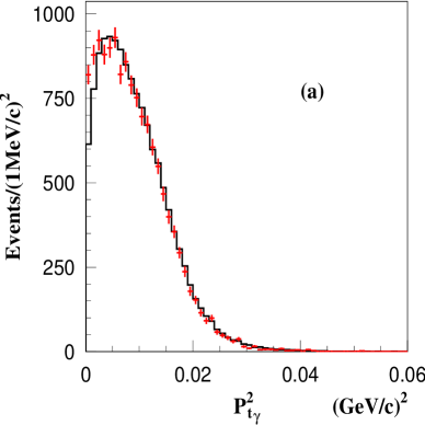
Figure 2: $P_{t\gamma}^{2}$ distributions. For (a), crosses are data, and the histogram is MC simulation of $J/\psi\rightarrow p\bar{p}\pi^{0}$. (b) Distribution for simulated $J/\psi\rightarrow\gamma p\bar{p}$ events. $P^{2}_{t\gamma}=4|\vec{P}_{miss}|^{2}\sin^{2}\theta_{\gamma}/2$ where $\vec{P}_{miss}$ is the missing momentum in the event determined using the two charged particles, and $\theta_{\gamma}$ is the angle between $\vec{P}_{miss}$ and the higher energy photon.

Figure 3: The $\gamma\gamma$ invariant mass spectrum of $J/\psi\rightarrow p\bar{p}\gamma\gamma$ candidates.

Figure 4: The invariant mass spectra of (a) $M_{p\pi^{0}}$ and (b) $M_{\bar{p}\pi^{0}}$ for $J/\psi\rightarrow p\bar{p}\pi^{0}$ candidate events, where the circles with error bars are the background events estimated from $\pi^{0}$ sideband events, and the black dots with error bars are those from simulated $J/\psi\rightarrow p\bar{p}\pi^{0}\pi^{0}$ events passing the selection criteria.

Figure 5: Dalitz plot of $J/\psi\rightarrow p\bar{p}\pi^{0}$ candidates.

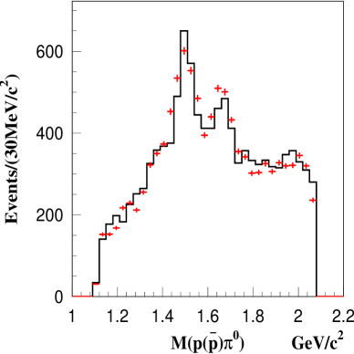
Figure 6: The re-normalized invariant mass spectra of $M_{p\pi^{0}}$ and $M_{\bar{p}\pi^{0}}$ after correction for detection efficiency, where the histogram is $M_{p\pi^{0}}$ and the crosses are $M_{\bar{p}\pi^{0}}$.

Other possible $J/\psi\to p\bar{p}\pi^{0}$ backgrounds are studied using MC simulation and data. Decay channels that have similar final states as $J/\psi\to p\bar{p}\pi^{0}$ are simulated, and $J/\psi\to p\bar{p}\pi^{0}\pi^{0}$ is found to be the main background channel. Surviving $J/\psi\rightarrow p\bar{p}\pi^{0}\pi^{0}$ events, passing all requirements described above, are plotted as black dots in Fig. 4. The invariant mass distribution of this background can be described approximately by phase space. The $\pi^{0}$ sideband, defined by $0.2<(M_{\gamma\gamma}-0.135)<0.2278$ GeV$/c^{2}$, is used to estimate the background from non-$\pi^{0}$ final states, such as $J/\psi\rightarrow\gamma p\bar{p}$, etc.. The circles in Fig. 4  show the contribution from $\pi^{0}$ sideband events. In the partial wave analysis, described below, two kinds of background are considered, $\pi^{0}$ sideband background and a non-interfering phase space background to account for the background from $J/\psi\rightarrow p\bar{p}\pi^{0}\pi^{0}$.

IV Partial wave analysis

A partial wave analysis (PWA) is performed to study the $N^{*}$ states in this decay. The sequential decay process can be described by $J/\psi\to\bar{p}N^{*}(p\bar{N}^{*})$, $N^{*}(\bar{N}^{*})\to p\pi^{0}(\bar{p}\pi^{0})$. The amplitudes are constructed using the relativistic covariant tensor amplitude formalism wrjs ; whl , and the maximum likelihood method is used in the fit.

IV.1 Introduction to PWA

The basic procedure for the partial wave analysis is the standard maximum likelihood method:
 (1) Construct the amplitude $A_{j}$ for the $j$-th possible partial wave in $J/\psi\rightarrow p\bar{N}_{X},\bar{N}_{X}\rightarrow\bar{p}\pi^{0}$ or $J/\psi\rightarrow\bar{p}N_{X},N_{X}\rightarrow p\pi^{0}$ as:

$$A_{j}=A_{prod-X}^{j}(BW)_{X}A_{decay-X},$$ (1)

where $A_{prod-X}^{j}$ is the amplitude which describes the production of the intermediate resonance $N_{X}$, $BW_{X}$ is the Breit-Wigner propagator of $N_{X}$, and $A_{decay-X}$ is the decay amplitude of $N_{X}$. The corresponding term for the $\bar{N}_{X}$ is obtained by charge conjugation with a negative sign due to negative C-parity of $J/\psi$.
 (2) The total transition probability, $\omega$, for each event is obtained from the linear combination of these partial wave amplitudes $A_{j}$ as $\omega=|\Sigma_{j}c_{j}A_{j}|^{2}$, where the $c_{j}$ parameters are to be determined by fitting the data.
 (3) The differential cross section is given by:

$$\frac{d\sigma}{d\Phi}=|\Sigma_{j}c_{j}A_{j}|^{2}+F_{bg},$$ (2)

where, $F_{bg}$ is the background function, which includes $\pi^{0}$ sideband background and non-interfering phase space background.
 (4) Maximize the following likelihood function $ln\cal L$ to obtain $c_{j}$ parameters, as well as the masses and widths of the resonances.

$${ln\cal L}=\sum\limits_{k=1}^{n}ln\frac{\omega(\xi_{k})}{\int d\xi\omega(\xi)\epsilon(\xi)},$$ (3)

where $\xi_{k}$ is the energy-momentum of the final state of the $k$-th observed event, $\omega(\xi)$ is the probability to generate the combination $\xi$, $\epsilon(\xi)$ is the detection efficiency for the combination $\xi$. As is usually done, rather than maximizing $\mathcal{L}$, $\mathcal{S}=-\rm{ln}\mathcal{L}$ is minimized.

For the construction of partial wave amplitudes, we assume the effective Lagrangian approach mbnc ; mgoet with the Rarita-Schwinger formalism wrjs ; cfncs ; suc3 ; suc2 . In this approach, there are three basic elements for constructing amplitudes: the spin wave functions for particles, the propagators, and the effective vertex couplings. The amplitude can then be written out by Feynman rules for tree diagrams.

For example, for $J/\psi\rightarrow\bar{N}N^{*}(\frac{3}{2}^{+})\rightarrow\bar{N}(\kappa_{1},s_{1})N(\kappa_{2},s_{2})\pi(\kappa_{3})$, the amplitude can be constructed as:

$$A_{\frac{3}{2}^{+}}= \bar{u}(\kappa_{2},s_{2})\kappa_{2\mu}P_{3/2}^{\mu\nu}(c_{1}g_{\nu\lambda}+c_{2}\kappa_{1\nu}\gamma_{\lambda}$$ (4)

$$+c_{3}\kappa_{1\nu}\kappa_{1\lambda})\gamma_{5}\upsilon(\kappa_{1},s_{1})\psi^{\lambda},$$

where $u(\kappa_{2},s_{2})$ and $\upsilon(\kappa_{1},s_{1})$ are $\frac{1}{2}$-spinor wave functions for $N$ and $\bar{N}$, respectively; $\psi^{\lambda}$ is the spin-1 wave function, $i.e.$, the polarization vector for $J/\psi$. The $c_{1}$, $c_{2}$, and $c_{3}$ terms correspond to three possible couplings for the $J/\psi\rightarrow\bar{N}N^{*}(\frac{3}{2}^{+})$ vertex. They can be taken as constant parameters or as smoothly varying vertex form factors. The spin $\frac{3}{2}^{+}$ propagator $P_{3/2+}^{\mu\nu}$ for $N^{*}(\frac{3}{2}^{+})$ is:

$$P_{3/2+}^{\mu\nu}= \frac{\gamma\cdot p+M_{N^{*}}}{M_{N^{*}}^{2}-p^{2}+iM_{N^{*}}\Gamma_{N^{*}}}[g^{\mu\nu}-\frac{1}{3}\gamma^{\mu}\gamma^{\nu}$$ (5)

$$-\frac{2p^{\mu}p^{\nu}}{3M_{N^{*}}^{2}}+\frac{p^{\mu}\gamma^{\nu}-p^{\nu}\gamma^{\mu}}{3M_{N^{*}}}],$$

with $p=\kappa_{2}+\kappa_{3}$. Other partial wave amplitudes can be constructed similarly wrjs ; whl .

The possible intermediate resonances are listed in Table 1. Of these states, only a few are (well) established states, while $N_{x}(1885)$ is one of the ‘missing’ $N^{*}$ states predicted by the quark model and not yet experimentally observed. $N_{x}(2065)$ is also a long-sought ‘missing’ $N^{*}$, which was observed recently by BES xbji .

For the lowest lying $N^{*}$ states, $N(1440)$, $N(1520)$, and $N(1535)$, Breit-Wigner’s with phase space dependent widths are used.

$$BW_{X}(s)=\frac{m\Gamma(s)}{s-m^{2}+im\Gamma(s)},$$ (6)

where $s$ is the invariant mass-squared. The phase space dependent widths can be written as tpv181 :

$$\Gamma_{N(1440)(s)}= \Gamma_{N(1440)}(0.7\frac{B_{1}(q_{\pi N})\rho_{\pi N}(s)}{B_{1}(q_{\pi N}^{N^{*}})\rho_{\pi N}(M_{N^{*}}^{2})}$$ (7)

$$+0.3\frac{B_{1}(q_{\pi\Delta})\rho_{\pi\Delta}(s)}{B_{1}(q_{\pi\Delta}^{N^{*}})\rho_{\pi\Delta}(M_{N^{*}}^{2})}),$$

$$\Gamma_{N(1520)}= \Gamma_{N(1520)}\frac{B_{2}(q_{\pi N})\rho_{\pi N}(s)}{B_{2}(q_{\pi N}^{N^{*}})\rho_{\pi N}(M_{N^{*}}^{2})},$$ (8)

$$\Gamma_{N(1535)}= \Gamma_{N(1535)}(0.5\frac{\rho_{\pi N}(s)}{\rho_{\pi N}(M_{N^{*}}^{2})}$$ (9)

$$+0.5\frac{\rho_{\eta N}(s)}{\rho_{\eta N}(M_{N^{*}}^{2})}),$$

where $B_{l}(q)$ ($l=1,2$) is the standard Blatt-Weisskopf barrier factor suc3 ; suc2 for the decay with orbital angular momentum $L$ and $\rho_{\pi N}(s)$, $\rho_{\pi\Delta}(s)$, and $\rho_{\eta N}(s)$ are the phase space factors for $\pi N$, $\pi\Delta$, and $\eta N$ final states, respectively.

$$\rho_{XY}(s)=\frac{2q_{XY}(s)}{\sqrt{s}},$$ (10)

$$q_{XY}(s)=\frac{\sqrt{(s-(M_{Y}+M_{X})^{2})(s-(M_{Y}-M_{X})^{2})}}{(2\sqrt{s})},$$ (11)

where $X$ is $\pi$ or $\eta$, $Y$ is $N$ or $\Delta$, and $q_{XY}(s)$ is the momentum of $X$ or $Y$ in the center-of-mass (CMS) system of $XY$. For other resonances, constant width Breit-Wigner’s are used.

As described in Ref. liangwh , the form factors are introduced to take into account the nuclear structure. We have tried different form factors, given in Ref. liangwh , in the analysis and find that for $J=\frac{1}{2}$ resonances, the form factor preferred in fitting is

$$F_{N}(s_{\pi N})=\frac{\Lambda_{N}^{4}}{\Lambda_{N}^{4}+(s_{\pi N}-m_{N^{*}}^{2})^{2}},$$ (12)

where $s_{\pi N}$ is the invariant mass squared of $N$, $\pi$, and for $J=\frac{3}{2}$ or $\frac{5}{2}$ states, the preferred form factor is

$$F_{N}(s_{\pi N})=e^{\frac{-|s_{N\pi}-m_{N^{*}}^{2}|}{\Lambda^{2}}}.$$ (13)

Therefore, the above form factors are used in this analysis.

In the log likelihood calculation, $\pi^{0}$ sideband background events are given negative weights; the sideband events then cancel background in the selected candidate sample. The $J/\psi\to p\bar{p}\pi^{0}\pi^{0}$ background is described by a non-interfering phase space term, and the amount of this background is floated in the fit.

Table 1: Resonances considered in the PWA analysis.

Resonance	Mass(MeV)	Width(MeV)	$J^{P}$	C.L.
$N(940)$	940	0	$\frac{1}{2}^{+}$	off-shell
$N(1440)$	1440	350	$\frac{1}{2}^{+}$	****
$N(1520)$	1520	125	$\frac{3}{2}^{-}$	****
$N(1535)$	1535	150	$\frac{1}{2}^{-}$	****
$N(1650)$	1650	150	$\frac{1}{2}^{-}$	****
$N(1675)$	1675	145	$\frac{5}{2}^{-}$	****
$N(1680)$	1680	130	$\frac{5}{2}^{+}$	****
$N(1700)$	1700	100	$\frac{3}{2}^{-}$	***
$N(1710)$	1710	100	$\frac{1}{2}^{+}$	***
$N(1720)$	1720	150	$\frac{3}{2}^{+}$	****
$N_{x}(1885)$	1885	160	$\frac{3}{2}^{-}$	‘missing’ $N^{*}$
$N(1900)$	1900	498	$\frac{3}{2}^{+}$	**
$N(2000)$	2000	300	$\frac{5}{2}^{+}$	**
$N_{x}(2065)$	2065	150	$\frac{3}{2}^{+}$	‘missing’ $N^{*}$
$N(2080)$	2080	270	$\frac{3}{2}^{-}$	**
$N(2090)$	2090	300	$\frac{1}{2}^{-}$	*
$N(2100)$	2100	260	$\frac{1}{2}^{+}$	*

IV.2 PWA results

Well established states, such as $N(1440)$, $N(1520)$, $N(1535)$, $N(1650)$, $N(1675)$, $N(1680)$ are included in this partial wave analysis. According to the framework of soft $\pi$ meson theory larfd , the off-shell decay process is also needed in this decay, and therefore $N(940)$ ($M=940$ MeV/c², $\Gamma$ = 0.0 MeV/c²) is also included. Fig. 7 shows the Feynman diagram for this process.

Figure 7: Feynman diagrams of $J/\psi\rightarrow p\bar{p}\pi^{0}$ for the off-shell decay process.

IV.2.1 Resonances in the 1.7 GeV/c² mass region

In the $M=1.7$ GeV/c² mass region, three resonances $N(1700)$($\frac{3}{2}^{-}$), $N(1710)$($\frac{1}{2}^{+}$), and $N(1720)$($\frac{3}{2}^{+}$) pdg are supposed to decay into $p\pi(\bar{p}\pi)$ final states. According to the Particle Data Group (PDG08) pdg , only $N(1720)$ is a well established state. We now study whether these three states are needed in $J/\psi\to p\bar{p}\pi^{0}$. This is investigated for two cases, first assuming no $N^{*}$ states in the high mass region ($>$ 1.8 GeV/c²), and second assuming $N_{x}(2065)$, $N(2080)$, and $N(2100)$ states in the high mass region. With no $N^{*}$ states in the $M>$ 1.8 GeV/c² mass region, the PWA shows that the significances of $N(1700)$ and $N(1720)$ are 3.2$\sigma$ ($\Delta S=11$) and 0.8$\sigma$ ($\Delta S=3$), and their fractions are 0.3% and 6%, respectively; only $N(1710)$ is significant. When $N_{x}(2065)$, $N(2080)$, and $N(2100)$ are included, the $N(1710)$ makes the log likelihood value $S$ better by 65, which corresponds to a significance much larger than 5$\sigma$. However, neither the $N(1700)$ nor the $N(1720)$ is significant. We conclude that the $N(1710)$ should be included in the PWA.

IV.2.2 $N_{x}(2065)$

The $N_{x}(2065)$, a long-sought ‘missing’ $N^{*}$ predicted by the quark model, was observed in $J/\psi\rightarrow p\bar{n}\pi^{-}+c.c.$ xbji with a mass of $2065\pm 3_{-30}^{+15}$ MeV/c² and a width of $175\pm 12\pm 40$ MeV/c², determined from a simple Breit-Wigner fit. We investigate the need for the $N_{x}(2065)$ in $J/\psi\to p\bar{p}\pi^{0}$. Including the $N(1440)$, $N(1520)$, $N(1535)$, $N(1650)$, $N(1675)$, $N(1680)$, $N(1710)$ and the off-shell decay in the PWA fit, different $N_{x}(2065)$ spin-parities ($J^{P}$) and different combinations of high mass resonances are tried. If there are no other resonances in the high mass region, the log likelihood value improves by 288, which corresponds to a significance of greater than $5\sigma$, when a $\frac{3}{2}^{+}$$N_{x}(2065)$ is added. Thus, the $N_{x}(2065)$ is definitely needed in this case, and its mass and width are optimized to be $M=2057_{-6}^{+4}$ MeV/c² and $\Gamma=220_{-12}^{+11}$ MeV/c².

The significance and spin-parity of $N_{x}(2065)$ is further checked under the following four hypotheses (A, B, C and D) for the high mass resonances. Case A has $N(2080)$ and $N(2100)$ included, case B $N(2080)$ and $N(2000)$, case C $N(2000)$, $N(2080)$, and $N(2100)$, and case D $N(2080)$, $N(2090)$, and $N(2100)$. The changes of the log likelihood values ($\Delta S$), the corresponding significances, and the fractions of $N_{x}(2065)$ are listed in Table  2 when a $\frac{3}{2}^{+}$ $N_{x}(2065)$ is added in the four cases. The log likelihood values become better by 58 to 126 when $N_{x}(2065)$ is included. Therefore, $N_{x}(2065)$ is needed all cases. The differences of log likelihood values for different $N_{x}(2065)$ $J^{P}$ assignments for the four combinations are listed in Table  3. The assignment of $J^{P}=\frac{3}{2}^{+}$ gives the best log likelihood value except for the cases where there is large interference. Spin-parity of $\frac{3}{2}^{+}$ is favored for $N_{x}(2065)$.

Table 2: Changes of log likelihood values ($\Delta S$), the corresponding significances, and the fractions of $N_{x}(2065)$, when $N_{x}(2065)$ is added in the four cases.

Case	$\Delta S$	significance	fraction (%)
A	126	$\gg$ 5$\sigma$	23
B	158	$\gg$ 5$\sigma$	24
C	79	$\gg$ 5$\sigma$	16
D	58	$\gg$ 5$\sigma$	22

Table 3: Comparison of log likelihood values for different $J^{P}$ assignments for $N_{x}(2065)$.

$J^{P}$	$\frac{1}{2}^{+}$	$\frac{1}{2}^{-}$	$\frac{3}{2}^{+}$	$\frac{3}{2}^{-}$	$\frac{5}{2}^{+}$	$\frac{5}{2}^{-}$
A	85.8	49.3	0.0	-32.2	-36.9	34.1
B	5.0	68.5	0.0	54.3	-12.1	6.3
C	98.1	39.8	0.0	85.6	76.1	14.4
D	44.2	45.2	0.0	25.0	36.2	38.0

IV.2.3 Other resonances in high mass region

In addition to the observed resonances, $N(2000)$, $N(2080)$, $N(2090)$ and $N(2100)$, as well as the $N_{x}(2065)$, there is another possible ‘missing’ $N^{*}$ state, $N_{x}(1885)$, which is predicted by theory but not yet observed.

a) $N_{x}(1885)$

In the $p(\bar{p})\pi^{0}$ invariant mass spectrum, shown in Fig. 4, no obvious peak is seen near 1.89 GeV/c². We study whether this state is needed in the partial wave analysis for the four cases. The significances are $1.3\sigma$ ($\Delta S=3.0$), $3.2\sigma$ ($\Delta S=8.8$), $3.4\sigma$ ($\Delta S=9.7$), and greater than $5\sigma$ ($\Delta S=28.0$) in cases A, B, C, and D, respectively, when a $N_{x}(1885)$ is included. Thus, the statistical significance is larger than 5$\sigma$ only in case D. In our final fit, $N_{x}(1885)$ is not included. However, the difference of including and not including it will be taken as a systematic error.

b) $N(2000)$, $N(2080)$, $N(2090)$, and $N(2100)$

We next study whether $N(2000)$, $N(2080)$, $N(2090)$ and $N(2100)$ are all significant in the decay. First, we add $N(2000)$, $N(2080)$, $N(2090)$, and $N(2100)$ one at a time with $N(940)$, $N(1440)$, $N(1520)$, $N(1535)$, $N(1650)$, $N(1675)$, $N(1680)$, $N(1710)$, and $N_{x}(2065)$ already included. The log likelihood values get better by 28, 137, 69, and 73, respectively, which indicates the $N(2080)$ is the most significant, all the significances are larger than $5\sigma$. Second, we include $N_{x}(2065)$ and $N(2080)$ in the high mass region and add the other three states $N(2000)$, $N(2090)$, and $N(2100)$ one at a time. The significances of the $N(2100)$ ($\Delta S=38$) and $N(2090)$ ($\Delta S=30$) are much larger than $5\sigma$, while $N(2000)$ is $3.9\sigma$ ($\Delta S=14$). Third, we include $N_{x}(2065)$, $N(2080)$, and $N(2100)$ in the high mass region and test whether $N(2000)$ and $N(2090)$ are needed again. The significances are larger than $5\sigma$ ($\Delta S=23$) and $2.7\sigma$ ($\Delta S=7$), respectively when $N(2000)$ and $N(2090)$ are included.

Due to the complexity of the high mass $N^{*}$ states and the limitation of our data, we are not able to draw firm conclusions on the high mass region. In the final fit, we include $N_{x}(2065)$, $N(2080)$, and $N(2100)$ and take the differences of with and without $N(2000)$ and $N(2090)$ as systematic errors.

IV.2.4 The best results up to now

We summarize the results we have so far:

(1) For the three resonances in the $M=1.7$ GeV/c² mass region ($N(1700)$, $N(1710)$, and $N(1720)$), only $N(1710)$ is significant.

(2) The $N_{x}(2065)$ is definitely needed in all cases, and its spin-parity favors $\frac{3}{2}^{+}$.

(3) $N_{x}(1885)$ is not significant and therefore is not included in the final fit.

(4) For other resonances in the high mass region, $N(2080)$ and $N(2100)$ are both needed in all cases tried, but the other two states $N(2000)$ and $N(2090)$ are not very significant and so are not included in the final fit.

Therefore, we consider $N(940)$, $N(1440)$, $N(1520)$, $N(1535)$, $N(1650)$, $N(1675)$, $N(1680)$, $N(1710)$, $N_{x}(2065)$, $N(2080)$, and $N(2100)$ in the fit.

Table 4 lists the optimized masses and widths for some $N^{*}$ resonances; the others are fixed to those from PDG08. Here, only statistical errors are indicated. The fractions of these states are also listed.

The $M_{p\pi^{0}}$ and $M_{\bar{p}\pi^{0}}$ invariant mass spectra and the angular distributions after the optimization are shown in Figs. 8 (a) and (b) and Fig. 9, respectively. In Fig. 8 and 9, the crosses are data and the histograms are the PWA fit projections. The PWA fit reasonably describes the data.

Table 4: Optimized masses and widths, as well as fractions. Errors shown are statistical only.

Resonance	Mass(MeV/c2)	Width(MeV/c2)	$J^{P}$	Fraction ($\%$)
$N(1440)$	$1455_{-7}^{+2}$	$316_{-6}^{+5}$	$\frac{1}{2}^{+}$	16.37
$N(1520)$	$1513_{-4}^{+3}$	$127_{-8}^{+7}$	$\frac{3}{2}^{-}$	7.96
$N(1535)$	$1537_{-6}^{+2}$	$135_{-8}^{+8}$	$\frac{1}{2}^{-}$	7.58
$N(1650)$	$1650_{-6}^{+3}$	$145_{-10}^{+5}$	$\frac{1}{2}^{-}$	9.06
$N(1710)$	$1715_{-2}^{+2}$	$95_{-1}^{+2}$	$\frac{1}{2}^{+}$	25.33
$N_{x}(2065)$	$2040_{-4}^{+3}$	$230_{-8}^{+8}$	$\frac{3}{2}^{+}$	23.39

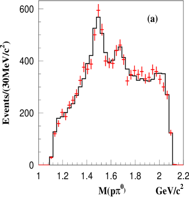
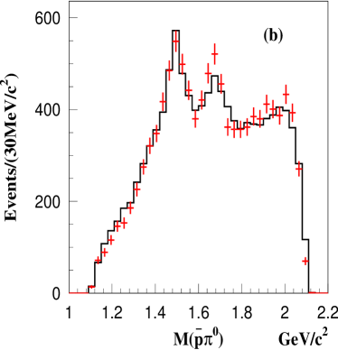
Figure 8: The $p\pi^{0}$ and $\bar{p}\pi^{0}$ invariant mass spectra after optimization of masses and widths. Plot (a) is $M_{p\pi^{0}}$, and plot (b) is $M_{\bar{p}\pi^{0}}$, where the crosses are data and histograms are fit results.

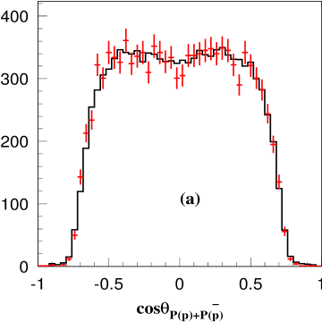
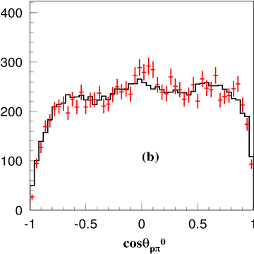
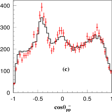
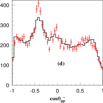
Figure 9: Distributions of (a) the cosine of the sum of the $p$ and $\bar{p}$ momenta, (b) cosine of the momentum of the ${p\pi^{0}}$ system in the $p\bar{p}$ CMS, (c) cosine of the momentum of the $p\bar{p}$ system in the $p\pi^{0}$ CMS, and (d) cosine of the momentum of $p\bar{p}$ in the $\bar{p}\pi^{0}$ CMS. The crosses are data and histograms are the fit results.

IV.2.5 $N_{x}(1885)$ significance with optimized $N^{*}$ states

In the analysis above, the $N_{x}(1885)$ was not found to be significant. Here its significance is redetermined using the optimized masses and widths for the $N^{*}$’s, and it is still only 1.2$\sigma$ ($\Delta S=2.7$). Therefore, we have the same conclusion: the $N_{x}(1885)$ is not needed.

IV.2.6 $N(1900)$

In PDG08 pdg , there is an $N(1900)$($\frac{3}{2}^{+}$) state near $N_{x}(2065)$ pdg . Our previous results show that if there is only one $\frac{3}{2}^{+}$ state in this region, the mass and width are optimized at $M=2057_{-6}^{+4}$ MeV/c² and $\Gamma=220_{-12}^{+11}$ MeV/c², which are consistent with those of $N_{x}(2065)$. If $N(1900)$ is also included in this analysis, i.e. there are two $\frac{3}{2}^{+}$ states in this region, we find that the second $\frac{3}{2}^{+}$ state also has a statistical significance much larger than 5$\sigma$ ($\Delta S=49$). However, the interference between $N(1900)$ and $N_{x}(2065)$ is about 80%. This analysis does not exclude the possibility that there are two $\frac{3}{2}^{+}$ states in this region.

IV.2.7 Search for additional $N^{*}$ and $\Delta^{*}$ resonances

Besides the contributions from the well-established $N^{*}$ resonances, there could be smaller contributions from other $N^{*}$ resonances and even $\Delta^{*}$ resonances from isospin violating virtual photon production.

What might be expected for the isospin violating decay? For the $J/\psi\rightarrow p\bar{p}$ decay, the isospin violating fraction can be estimated using the PDG $J/\psi$ leptonic branching fraction and the proton electromagnetic form factor $F_{p}(q^{2})$baub to be $B(J/\psi\rightarrow\gamma^{*}\rightarrow p\bar{p})$ = $B(J/\psi\rightarrow l^{+}l^{-})\times(F_{p}(M_{J/\psi}^{2})^{2}$ = $2.4\times 10^{-5}$. The total $J/\psi\rightarrow p\bar{p}$ branching fraction is $2.2\times 10^{-3}$pdg . This means, the fraction of decays through a virtual photon in the $J/\psi\rightarrow\gamma^{*}\rightarrow p\bar{p}$ decay mode is close to 1.1%. For the non-strange channel, the ratio of photon couplings to isospin 1 and isospin 0 is 9:1, so the isospin violating part is about 1% for this channel. For the $J/\psi\rightarrow p\bar{p}\pi^{0}$ decay, one would expect a similar isospin violating fraction.

If we add an extra state with different possible spin-parities ($J^{P}=\frac{1}{2}^{\pm},\frac{3}{2}^{\pm},\frac{5}{2}^{\pm}$) in the large mass (1.65 GeV/c² to 1.95 GeV/c²) region with widths from 0.05 GeV/c² to 0.20 GeV/c² and re-optimize, we find that no additional $N^{*}$’s or $\Delta^{*}$’s with the statistical significance of greater than 5$\sigma$ are required.

IV.2.8 Search for $\rho(2150)$

A resonance with mass 2149 MeV/c² and $J^{P}=1^{-}$ is listed in PDG08 pdg with the decay $\rho(2150)\rightarrow p\bar{p}$. Here, we test whether there is evidence for this decay in our sample. The significance of this resonance is less than 3$\sigma$ when we vary the width of this state in the fit from 200 to 660 MeV/c². Therefore, our data do not require this state. Figure 10 shows the $p\bar{p}$ invariant mass spectrum, and there is no clear structure near 2149 MeV/c².

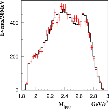
Figure 10: The $p\bar{p}$ invariant mass spectra. Crosses are data and histogram is the PWA fit after the optimization of masses and widths.

V Branching fraction of $J/\psi\to p\bar{p}\pi^{0}$

The branching fraction of $J/\psi\to p\bar{p}\pi^{0}$ is obtained by fitting the $\pi^{0}$ signal (see Fig. 3) with a $\pi^{0}$ shape obtained from $J/\psi\rightarrow p\bar{p}\pi^{0}$ MC simulation and a polynomial background. The numbers of fitted signal and background events are 11,166 and 691, respectively. The efficiency of $J/\psi\to p\bar{p}\pi^{0}$ is determined to be 13.77% by MC simulation with all intermediate $N^{*}$ states being included. Figures 11 (a) and (b) show the $p$ and $\bar{p}$ momentum distributions, where the histograms are MC simulation of $J/\psi\rightarrow p\bar{p}\pi^{0}$ using the $J^{P}$’s and fractions of $N^{*}$ states obtained from our partial wave analysis, and the crosses are data. There is good agreement between data and MC simulation.

The branching fraction is determined to be:

$$Br(J/\psi\rightarrow p\bar{p}\pi^{0})=(1.33\pm 0.02~{}(stat.))\times 10^{-3},$$ (14)

which is higher than that in PDG08 pdg ($(1.09\pm 0.09)\times 10^{-3}$).

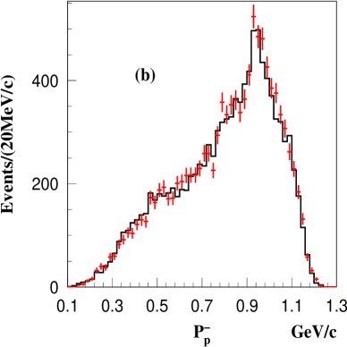
Figure 11: Momentum distributions of $p$ and $\bar{p}$ in $J/\psi\rightarrow p\bar{p}\pi^{0}$, where histograms are $J/\psi\rightarrow p\bar{p}\pi^{0}$ MC simulation using the spin parities and fractions of $N^{*}$ states obtained from our partial wave analysis and crosses are data.

VI Systematic errors

The systematic errors for the masses and widths of $N^{*}$ states mainly originate from the difference between data and MC simulation, the influence of the interference between $N(2100)$ and other states, uncertainty of the background, the form-factors, and the influence of high mass states, as well as the differences when small components are included or not.

(1) Two different MDC wire resolution simulation models are used to estimate the systematic error from the data/MC difference.

(2) In this analysis, the interference between $N(2100)$($\frac{1}{2}^{+}$) and the low mass regions states such as $N(940)$($\frac{1}{2}^{+}$) and $N(1440)$($\frac{1}{2}^{+}$) can be very large, even larger than 50%. We fix the fraction of $N(2100)$ to be less than 10% to reduce the interference and then compare its impact on other resonances. The biggest differences for the masses, widths, and fractions of the other resonances between fixing the fraction of $N(2100)$ and floating its fraction are considered as systematic errors.

(3) Two kinds of backgrounds are considered in the partial wave analysis, $\pi^{0}$ sideband and non-interfering phase space. We increase the number of background events by 10%, and take the changes of the optimized masses and widths as systematic errors.

(4) Equations (12) and (13) are the form factors used in this analysis, where $\Lambda$ is 2.0 for $N^{*}$ states with $J^{P}=\frac{1}{2}$ and $\Lambda$ is 1.2 for those with $J^{P}=\frac{3}{2}$ and $\frac{5}{2}$. Other form factors have also been tried, however their log likelihood values are much worse than those from the form factors used here. We also vary the $\Lambda$ values from 2.0 and 1.2 to 1.5. The biggest differences are taken as the form factor systematic errors.

(5) The effect of using different combinations of states in the high mass region on the masses and widths of other resonances was investigated above (see Table 2), and the differences also taken as systematic errors.

Table 5 shows the summary of the systematic errors for the masses and widths, and the total systematic errors are the sum of each source added in quadrature.

Table 5: Summary of the systematic errors for masses and widths of $N^{*}$ resonances (MeV/c²).

Systematic error	$N(1440)$		$N(1520)$		$N(1535)$		$N(1650)$		$N(1710)$		$N_{x}(2065)$
	$\Delta M$	$\Delta\Gamma$	$\Delta M$	$\Delta\Gamma$	$\Delta M$	$\Delta\Gamma$	$\Delta M$	$\Delta\Gamma$	$\Delta M$	$\Delta\Gamma$	$\Delta M$	$\Delta\Gamma$
Data/MC comparison	3	14	2	13	2	11	4	12	1	12	1	19
Interference	12	25	2	23	3	22	25	15	15	2	10	20
Background uncertainty	18	51	11	23	6	28	2	8	4	10	5	15
Different form-factors	12	25	2	5	8	1	3	5	15	22	20	14
Different combinations in high mass region	35	21	7	12	5	10	5	23	20	35	10	39
Total	43	67	13	37	12	39	26	31	29	44	25	52

Table 6: Systematic error for the branching fraction $B(J/\psi\to\pi^{0}p\bar{p})$ from different sources.

Sys. error sources	Systematic error(%)
Wire resolution	2.18
Photon efficiency	4.00
Particle ID	4.00
Mass spectrum fitting	1.93
Number of $J/\psi$ events	4.72
Total	7.93

Table 7: Summary of $N^{*}$ states optimized results.

Resonance	Mass(MeV/c2)	width(MeV/c2)	$J^{P}$	Fraction(%)	Branching fraction ($\times 10^{-4}$)
$N(1440)$	$1455_{-7}^{+2}\pm 43$	$316_{-6}^{+5}\pm 67$	$\frac{1}{2}^{+}$	9.74$\sim$25.93	1.33$\sim$3.54
$N(1520)$	$1513_{-4}^{+3}\pm 13$	$127_{-8}^{+7}\pm 37$	$\frac{3}{2}^{-}$	2.38$\sim$10.92	0.34$\sim$1.54
$N(1535)$	$1537_{-6}^{+2}\pm 12$	$135_{-8}^{+8}\pm 39$	$\frac{1}{2}^{-}$	6.83$\sim$15.58	0.92$\sim$2.10
$N(1650)$	$1650_{-6}^{+3}\pm 26$	$145_{-10}^{+5}\pm 31$	$\frac{1}{2}^{-}$	6.89$\sim$27.94	0.91$\sim$3.71
$N(1710)$	$1715_{-2}^{+2}\pm 29$	$95_{-1}^{+2}\pm 44$	$\frac{1}{2}^{+}$	4.17$\sim$30.10	0.54$\sim$3.86
$N_{x}(2065)$	$2040_{-4}^{+3}\pm 25$	$230_{-8}^{+8}\pm 52$	$\frac{3}{2}^{+}$	7.11$\sim$24.29	0.91$\sim$3.11

The systematic errors for the branching fraction $B(J/\psi\to\pi^{0}p\bar{p})$ mainly originate from the data/MC discrepancy for the tracking efficiency, photon efficiency, particle ID efficiency, fitting region used, the background uncertainty, and the uncertainty in the number of $J/\psi$ events.

(1) The systematic error from MDC tracking and the kinematic fit, 2.18%, is estimated by using different MDC wire resolution simulation models.

(2) The photon detection efficiency has been studied using $J/\psi\rightarrow\rho\pi$ smli . The efficiency difference between data and MC simulation is about 2% for each photon. So 4% is taken as the systematic error for two photons in this decay.

(3) A clean $J/\psi\rightarrow p\bar{p}\pi^{+}\pi^{-}$ sample is used to study the error from proton identification. The error from the proton PID is about 2%. So the total error from PID is taken as 4% in this decay.

(4) The $\pi^{0}$ fitting range is changed from 0.04 - 0.3 GeV/c² to 0.04 - 0.33 GeV/c², and the difference , 1.28%, is taken to be the systematic error from the fitting range. To estimate the uncertainty from the background shape, we change the background shape from 3rd order polynomial to other functions. The biggest change, 1.44%, is taken as the systematic error.

(5) The total number of $J/\psi$ events determined from inclusive 4-prong hadrons is $(57.70\pm 2.72)\times 10^{6}$ fangss . The uncertainty is 4.72%.

Table 6 lists the different sources of systematic errors for the branching fraction of $J/\psi\rightarrow p\bar{p}\pi^{0}$. The total systematic error is the sum of each error added in quadrature.

VII Summary

Based on 11,166 $J/\psi\rightarrow p\bar{p}\pi^{0}$ candidates from $5.8\times 10^{7}$ BESII $J/\psi$ events, a partial wave amplitude analysis is performed. A long-sought ‘missing’ $N^{*}$, which was observed first by BESII in $J/\psi\to p\bar{n}\pi^{-}+c.c.$, is also observed in this decay with mass and width of $2040_{-4}^{+3}\pm 25$ MeV/c² and $230_{-8}^{+8}\pm 52$ MeV/c², respectively. The mass and width obtained here are consistent with those from $J/\psi\to p\bar{n}\pi^{-}+c.c.$ within errors. Its spin-parity favors $\frac{3}{2}^{+}$. The masses and widths of other $N^{*}$ resonances in the low mass region are also obtained and listed in Table 7, where the first errors are statistical and the second are systematic. The ranges for the fractions of $N^{*}$ states, and thus the branching fractions, are given too. From this analysis, we find that the fractions of each $N^{*}$ state depend largely on the $N^{*}$’s used in the high mass region, the form factors, and Breit-Wigner parameterizations, as well as the background. We also determine the $J/\psi\to p\bar{p}\pi^{0}$ branching fraction to be $Br(J/\psi\rightarrow p\bar{p}\pi^{0})=(1.33\pm 0.02\pm 0.11)\times 10^{-3}$, where the efficiency used includes the intermediate $N^{*}$ and $\bar{N}^{*}$ states obtained in our partial wave analysis.

VIII Acknowledgments

The BES collaboration thanks the staff of BEPC and computing center for their hard efforts. This work is supported in part by the National Natural Science Foundation of China under contracts Nos. 10491300, 10225524, 10225525, 10425523, 10625524, 10521003, 10821063, 10825524, the Chinese Academy of Sciences under contract No. KJ 95T-03, the 100 Talents Program of CAS under Contract Nos. U-11, U-24, U-25, and the Knowledge Innovation Project of CAS under Contract Nos. U-602, U-34 (IHEP), the National Natural Science Foundation of China under Contract Nos. 10775077, 10225522 (Tsinghua University), and the Department of Energy under Contract No. DE-FG02-04ER41291 (U. Hawaii).

References

- (1) N. Isgur, nucl-th/0007008 (2000).
- (2) E. G. Cazzoli, Phys. Rev. Lett. 34, 1125 (1975).
- (3) S. E. Csorna et al., Phys. Rev. Lett., 86, 4243 (2001).
-
(4)
B. Aubert (BABAR Colaboration), Phys. Rev. D 72, 052006 (2005).
B. Aubert (BABAR Colaboration), hep-ex/0607042.
B. Aubert (BABAR Colaboration), Phys. Rev. Lett., 97, 232001 (2006).
B. Aubert (BABAR Colaboration), Phys. Rev. D 74, 011103 (2006).
B. Aubert (BABAR Colaboration), hep-ex/0607086.
B. Aubert (BABAR Colaboration), Phys. Rev. Lett., 98, 012001 (2007).
B. Aubert (BABAR Colaboration), Phys. Rev. D 77, 012002 (2009).
-
(5)
K. Abe (BELLE Collaboration), Phys. Rev. Lett., 98, 262001 (2007).
R. Chistov (BELLE Collaboration), Phys. Rev. Lett., 97, 162001 (2006).
R. Mizuk (BELLE Collaboration), Phys. Rev. Lett., 94, 122002 (2005). - (6) M. Iori et al., hep-ex/0701021.
- (7) C. Amsler et al., Phys. Lett. B 667, 1 (2008).
-
(8)
G. Bari, et al., Nuovo Cim., A 104, 1787 (1991).
G. Bari, et al., Nuovo Cim., A 104, 571 (1991). -
(9)
T. Aaltonen (CDF Collaboration), Phys. Rev. Lett., 99, 202001 (2007).
T. Aaltonen (CDF Collaboration), Phys. Rev. Lett., 99, 052002 (2007). -
(10)
V. M. Abazov (D0 Collaboration), Phys. Rev. Lett., 99, 052001 (2007).
V. M. Abazov (D0 Collaboration), arXiv:0808.4142. - (11) B. Aubert et al., Phys. Rev. D73, 012005 (2006).
- (12) C. Amsler et al., Physics Lett. B667, 1 (2008).
- (13) S. Capstick and W. Roberts, Prog. Part. Nucl. Phys. 45, S241 (2000).
- (14) N. Isgur and G. Karl, Phys. Rev. D19, 2653 (1979).
- (15) S. Capstick and W. Roberts, Phys. Rev. D47, 1994 (1993).
- (16) J. Z. Bai et al. (BES Collaboration), Phys. Lett. B510, 75 (2001).
- (17) M. Ablikim et al. (BES Collaboration), Phys. Rev. Lett. 97, 062001 (2006).
- (18) J. Z. Bai et. al, (BES Collab.), Nucl. Inst. and Meths. A458, 627 (2001).
- (19) M. Ablikim et al. (BES Collaboration), Nucl. Instrum. Meth. A552, 344 (2005).
- (20) W. Rarita and J. Schwinger, Phys. Rev. 60, 61 (1941).
- (21) W. H. Liang, P. N. Shen, J. X. Wang and B. S. Zou, J. Phys. G28, 333 (2002).
- (22) S. U. Chung, Phys. Rev. D48, 1225 (1993).
- (23) M. Benmerrouche, N. C. Mukhopadhyay and J. F. Zhang, Phys. Rev. Lett. 77, 4716 (1996); Phys. Rev. D51, 3237 (1995).
- (24) M. G. Olsson and E. T. Osypowski, Nucl. Phys. B87, 399 (1975); Phys. Rev. D17, 174 (1978); M. G. Olsson, E. T. Osypowski and E. H. Monsay, Phys. Rev D17,2938 (1978).
- (25) C. Fronsdal, Nuovo Cimento Sppl. 9, 416 (1958); R. E. Behrends and C. Fronsdal, Phys. Rev. 106, 345 (1957).
- (26) S. U. Chung, Spin Formalisms, CERN Yellow Report 71-8 (1971); S. U. Chung, Phys. Rev. D48, 1225 (1993); J. J. Zhu and T. N. Ruan, Communi. Theor. Phys. 32, 293, 435 (1999).
- (27) L. Adler and R. F. Dashen, Current Algebra and Application to Particle Physics (Benjamin, New York, 1968); B. W. Lee, Chiral Dynamics (Gordon and Breach, New York, 1972).
- (28) T. P. Vrana, S. A. Dytman and T. S. H. Lee, Phys. Rept. 328, 181 (2000).
- (29) Liang Wei-hong. Ph.D thesis, Institute of High Energy Physics, Chinese Academy of Science, 2002 (in Chinese); G.Penner and U. Mosel, Phys. Rev. C66, 055211 (2002); W. H. Liang et al., Eur. Phys. J. A21, 487 (2004).
- (30) S. M. Li et al., HEP NP 28, 859 (2004) (in Chinese).
- (31) Fang S.S. et al., HEP NP 27, 277 (2003) (in Chinese).