Authors:

RAUL ALEJANDRO AVALOS-ZUÑIGA

Universidad Autónoma Metropolitana-Iztapalapa. Av. San Rafael Atlixco 186, col. Vicentina, 09340 D.F. México. Tel.: +52 55 5804 4648 ext. 238. Fax: +52 55 5804 4900. E-mail: raaz@xanum.uam.mx.

MINGTIAN XU

Forschungszentrum Dresden-Rossendorf, P.O. Box 510119, 01314 Dresden, Germany. Tel.: +49 351 260 2227. Fax: +49 351 260 2007. E-mail:M.Xu@fzd.de

FRANK STEFANI

Forschungszentrum Dresden-Rossendorf, P.O. Box 510119, 01314 Dresden, Germany. Tel.: +49 351 260 3069. Fax: +49 351 260 2007. E-mail: F.Stefani@fzd.de

GUNTER GERBETH

Forschungszentrum Dresden-Rossendorf, P.O. Box 510119, 01314 Dresden, Germany. Tel.: +49 351 260 2168. Fax: +49 351 260 2007. E-mail:G.Gerbeth@fzd.de

FRANCK PLUNIAN

Laboratoire de Géophysique Interne et de Tectonophysique, BP 53, 38041 Grenoble Cedex 9, France. Tel.: +33 4 76 82 80 37. Fax: 33 4 76 82 81 01. E-mail: Franck.Plunian@ujf-grenoble.fr

Cylindrical anisotropic $\alpha^{2}$ dynamos

$\dagger$Forschungszentrum Dresden-Rossendorf, P.O. Box 510119, 01314 Dresden, Germany
$\ddagger$Lab. de Géophysique Interne et de Tectonophysique, BP 53, 38041 Grenoble Cedex 9, France
(Received 30 November 2006; in final form 15 June 2007)

We explore the influence of geometry variations on the structure and the time-dependence of the magnetic field that is induced by kinematic $\alpha^{2}$ dynamos in a finite cylinder. The dynamo action is due to an anisotropic $\alpha$ effect which can be derived from an underlying columnar flow. The investigated geometry variations concern, in particular, the aspect ratio of height to radius of the cylinder, and the thickness of the annular space to which the columnar flow is restricted. Motivated by the quest for laboratory dynamos which exhibit Earth-like features, we start with modifications of the Karlsruhe dynamo facility. Its dynamo action is reasonably described by an $\alpha^{2}$ mechanism with anisotropic $\alpha$ tensor. We find a critical aspect ratio below which the dominant magnetic field structure changes from an equatorial dipole to an axial dipole. Similar results are found for $\alpha^{2}$ dynamos working in an annular space when a radial dependence of $\alpha$ is assumed. Finally, we study the effect of varying aspect ratios of dynamos with an $\alpha$ tensor depending both on radial and axial coordinates. In this case only dominant equatorial dipoles are found and most of the solutions are oscillatory, contrary to all previous cases where the resulting fields are steady.

Keywords: Dynamo; $\alpha$ effect; magnetic field orientation

1 Introduction

It is generally assumed that columnar flows in the Earth’s outer core play an essential role for the generation of the geomagnetic field. At the surface of the Earth, the magnetic field structure has almost an axial dipole (AD) structure closely aligned with the Earth’s rotation axis. Direct numerical simulations of the geodynamo have successfully reproduced many observed features like, e.g., the dominance of the axial dipole and the occurrence of reversals (e.g. Olson et al. 1999, Ishihara and Kida 2002, Aubert and Wicht 2004, Wicht and Olson 2004 and references therein). The poloidal part of the field is thought to be produced from the toroidal part by the $\alpha$-effect generated by the columnar flows, while the toroidal component of the Earth’s magnetic field is associated to the $\Omega$-effect, but also again to an $\alpha$-effect or even to both mechanisms together. These types of magnetic field generation are usually referred to as $\alpha\Omega$, $\alpha^{2}$ and $\alpha^{2}\Omega$ dynamos, respectively.

It was one of the motivations of the Karlsruhe dynamo experiment to study an Earth-like magnetic field generation process in the laboratory (Gailitis 1967, Busse 1975, Stieglitz and Müller 2001). However, in contrast to the axial dipole (AD) of the Earth, the eigenfield structure of the Karlsruhe dynamo is an equatorial dipole (ED) what has been predicted in terms of the mean-field theory with an anisotropic $\alpha$ effect (Rädler et al. 1998). Actually, a general tendency of anisotropic $\alpha^{2}$ dynamos to produce fields with dominant equatorial dipole structure has been known for long (Rädler 1975, Rädler 1980, Rüdiger 1980, Rüdiger and Elstner 1994).

It is also well known that a transition from equatorial to axial dipoles can occur if some differential rotation is added (Rädler 1986, Gubbins et al. 2000). However, an axial field orientation can also result from $\alpha^{2}$ dynamos if the magnetic diffusion is enhanced by small scales of the flow (Tilgner 2004).

Besides the axial and equatorial dipole, the quadrupole structure seems to play also a certain role in geodynamo models. In many kinematic models one finds a quasi-degeneration with the dipole field (Gubbins et al. 2000). This degeneration is also responsible for the appearance of hemispherical dynamos in dynamically coupled models (Grote and Busse 2000). In this case, both quadrupolar and dipolar components contribute nearly equal magnetic energy so that their contributions cancel in one hemisphere and add to each other in the opposite hemisphere. The interplay between the nearly degenerated (Gubbins et al. 2000) axial dipole, equatorial dipole, and quadrupole was used in various models to explain the reversal phenomenon of the geodynamo (Melbourne et al. 2001).

With the same focus on field reversals, the importance of transitions between steady and oscillatory solutions of kinematic dynamos has been highlighted by several authors (Weisshaar 1982, Yoshimura et al. 1984, Sarson and Jones 1999, Phillips 1993, Rüdiger et al. 2003). In an extremely reduced reversal model dealing only with the axial dipole it was shown that many features of reversals (typical time scales, asymmetry between slow dipole decay and fast recovery, bimodal field distribution) can be understood by the magnetic field dynamics in the vicinity of transition points between steady and oscillatory solutions (Stefani and Gerbeth 2005, Stefani et al. 2006a, Stefani et al. 2006b). The main ingredient of this reversal model, as well as of the reversal model of Giesecke et al. (Giesecke et al. 2005a), is a sign change of $\alpha$ along the radius which brings into play a coupling between the first two radial eigenfunctions of the axial dipole field. It should be noticed that such a sign change results indeed from simulations of magneto-convection (Giesecke et al. 2005b).

With this background, we investigate in the present paper various kinematic dynamo models within cylindrical geometry. Our focus will lay first on the dominance of field structure: equatorial (ED) or axial dipoles (AD) or even quadrupoles (Q), and second on the occurrence of oscillatory solutions. The cylindrical geometry, which might seem awkward from the purely geodynamo perspective, is quite natural from an experimentalist’s viewpoint. One could ask, e.g., how the geometry and the arrangement of spin-generators in the Karlsruhe dynamo could be modified in order to make its eigenfield prone to reversals.

After presenting the general framework, we will explore geometrical effects that could lead to dominant AD fields in cylindrical anisotropic $\alpha^{2}$ dynamos. The utilised numerical code, which is based on the integral equation approach to kinematic dynamos (Stefani et al. 2000, Xu et al. 2004a, Xu et al. 2004b, Xu et al. 2006), was already used for the simulation of various cylindrical dynamos, including the VKS dynamo experiment in Cadarache (Stefani et al. 2006c).

The geometrical variations which are actually considered are the aspect ratio of height to radius of the cylinder and the width of the annular space to which the dynamo source is restricted. First we consider the geometry of the Karlsruhe dynamo experiment. Its steady dynamo field is generated by a bundle of axially invariant helical columns, which is well described within mean-field theory as an $\alpha^{2}$ dynamo with anisotropic $\alpha$-effect. We find that for this experiment a dominant AD field could be achieved below a critical value of the aspect ratio which is not so far from the one of the real facility. In a next step, we explore more complex structures of $\alpha$ which have been derived from a flow described by axially invariant helical columns which are restricted to an annular space. The resulting $\alpha$ coefficients acquire a radial profile which depends on the flow structure. As for the modified Karlsruhe case, dynamo solutions show dominant steady AD fields below a critical value of the aspect ratio. In contrast to this, the reduction of the thickness of the annular space does not lead to a transition from non-axisymmetric to axisymmetric modes, although the critical dynamo numbers for both modes seem to converge. Finally, we have considered axial-radial dependence of $\alpha$. The dynamo action works in a fixed annular space and again the aspect ratio of height to radius of cylinder is the varying geometrical parameter. In this case, non-axisymmetric oscillatory fields are the dominant solutions.

2 The general concept

We consider an incompressible steadily moving fluid with velocity $\mathrm{\mathbf{u}}$, which is confined to a cylinder and surrounded by vacuum. The fluid has homogenous electrical conductivity $\sigma$ and magnetic permeability $\mu$. The fluid motion induces a magnetic field $\mathrm{\mathbf{B}}$ which extends in whole space. The magnetic field is governed by the induction equation

$$\eta\nabla^{2}\,\mathrm{\mathbf{B}}+\nabla\times(\mathrm{\mathbf{u}}\times\mathrm{\mathbf{B}})-\partial_{t}\,\mathrm{\mathbf{B}}=\bf 0\,,\quad\nabla\cdot\mathrm{\mathbf{B}}=0\,,$$ (1)

where $\eta$ is the magnetic diffusivity defined by $\eta=1/\mu\sigma$. In the mean field approach, each quantity is decomposed into a mean part (denoted by an overline) and a fluctuating part (denoted by a prime). Referring to a cylindrical coordinate system $(s,\varphi,z)$, we define mean fields by averaging over $\varphi$.

As we are only interested in the induction effects originated by the fluctuating part $\mathrm{\mathbf{u}}^{\prime}$ we assume that the mean motion $\overline{\mathrm{\mathbf{u}}}$ is equal to zero. In this case, the mean part of the induction equation (1) reduces to

$$\eta\nabla^{2}\,\overline{\mathrm{\mathbf{B}}}+\nabla\times{\mbox{\boldmath$\cal{E}$}}-\partial_{t}\,\overline{\mathrm{\mathbf{B}}}=\bf 0\,,\quad\nabla\cdot\overline{\mathrm{\mathbf{B}}}=0\,,$$ (2)

where ${\mbox{\boldmath$\cal{E}$}}=\overline{\mathrm{\mathbf{u}}^{\prime}\times\mathrm{\mathbf{B}}^{\prime}}$, is the mean electromotive force (e.m.f.) which is the source of generation of the large scale magnetic field $\overline{\mathrm{\mathbf{B}}}$. This e.m.f. results from the interaction of motion and magnetic field at small scales.

2.1 Representations of $\cal{E}$

We consider different forms of $\cal{E}$ which are generated by flows organised in columnar vortices parallel to the vertical axis of the cylinder. In the following only the $\alpha$ effect that results from these columnar structures is considered as the main contribution to the generation of $\cal{E}$, other effects are just neglected. In a strict sense, such a reduction of $\cal{E}$ to an $\alpha$-effect term is only possible if the spatial variations of $\overline{\mathrm{\mathbf{B}}}$ are sufficiently weak.

We consider first the mean e.m.f $\cal{E}$ produced by the flow in the Karlsruhe dynamo experiment (Rädler et al. 1998 ). Its most simplified analytical representation is given by

$$\begin{array}[]{ccc}{\mbox{\boldmath$\cal{E}$}}&=&-\alpha\left(\,\overline{\mathrm{\mathbf{B}}}-(\mathrm{\mathbf{e}}_{z}\cdot\overline{\mathrm{\mathbf{B}}}\,)\mathrm{\mathbf{e}}_{z}\right).\end{array}$$ (3)

where $\alpha$ is constant in the cylindrical volume and ${{\mbox{\boldmath$e$}}}_{z}$ is the unit vector in axial direction. We point out the anisotropy of the $\alpha$-effect as represented in (3).

The next considered example of $\cal{E}$ results from an axially invariant flow organised in columnar vortices equally distributed in an annular region. Similar flow structures were recently discussed in the context of quasi-geostrophic dynamos (Schaeffer and Cardin 2006). A detailed description of such ”rings of rolls” and the $\alpha$ tensor resulting from them has been derived by Avalos et al. (2007) and is given in Appendix A. The mean e.m.f. $\cal{E}$ produced by such a flow is given, under the assumptions mentioned in Appendices A and B, by

$${\mathcal{{E}}}_{\kappa}=\alpha_{\kappa\lambda}(s)\,\overline{B}_{\lambda},$$ (4)

with the subscripts $\kappa$ and $\lambda$ standing for $s$, $\varphi$, or $z$.

For some flow configurations, it has been shown (Avalos et al. 2007) that the resulting matrix $\alpha_{\kappa\lambda}$ is of the form

$$\alpha_{\kappa\lambda}=\left\{\begin{array}[]{ccc}\alpha_{ss}(s)&0&0\\ 0&\alpha_{\varphi\varphi}(s)&0\\ 0&\alpha_{z\varphi}(s)&0\end{array}\right\}.$$ (5)

We have also considered an additional axial dependence of the components in (5) multiplying them by harmonic functions of $z$ that vanish at the top and the bottom of the cylinder. This was motivated by the fact that for rolls in real rotating bodies a North-South antisymmetry of the axial velocity is expected, while the horizontal velocity components are expected to be symmetric with respect to the equator. Admittedly, the correct treatment of this problem would require a new derivation of the $\alpha$ matrix for such rolls along the lines outlined in the appendices. As a sort of compromise we focus here only on the general symmetry properties of the elements of the $\alpha$ matrix. Since $\alpha_{ss}$ and $\alpha_{\varphi\varphi}$ depend on products of axial and horizontal velocity components, we expect an antisymmetric behaviour. On the other hand, $\alpha_{z\varphi}$ should remain North-South symmetric since it depends on horizontal velocity components only.

The cylinder is assumed to extend over the axial interval $-H/2\leq z\leq H/2$. If we assume $u_{s}$ and $u_{\varphi}$ to be proportional to $\cos(\pi z/H)$ and $u_{z}$ to be proportional to $\sin(2\pi z/H)$, then the new $\alpha$ matrix is given by

$$\alpha_{\kappa\lambda}=\left\{\begin{array}[]{ccc}\alpha_{ss}(s)\cos(\pi z/H)\sin(2\pi z/H)&0&0\\ 0&\alpha_{\varphi\varphi}(s)\cos(\pi z/H)\sin(2\pi z/H)&0\\ 0&\alpha_{z\varphi}(s)\cos^{2}(\pi z/H)&0\end{array}\right\}.$$ (6)

Evidently, the resulting diagonal elements of $\alpha_{\kappa\lambda}$ are anti-symmetric with respect to $z=0$, whereas the non-diagonal element is symmetric with respect to $z=0$.

Though the representation of $\cal{E}$ defined above was derived for an infinitely extended conducting fluid, we assume that it applies also to a finite cylinder. This approximation has been successfully used, e.g. in Rädler et al. (1998, 2002), to solve the Karlsruhe dynamo problem in a finite cylinder. In this case the symmetry of the most easily excited magnetic field mode was found to be independent of the conductivity outside the cylinder, while the other properties of this mode well depend on the conductivity in outer space.

3 Dynamo solutions

Once we have defined different representations of $\cal{E}$, we solve the mean-field dynamo problem in a finite cylinder enclosed by vacuum using a numerical code based on the integral equation approach (Stefani et al. 2000, Xu et al. 2004a, Xu et al. 2004b, Xu et al. 2006).The magnetic field is determined by a self-consistent solution of the Biot-Savart equation together with a surface integral equation for the electric potential at the vacuum boundaries. For time-dependent solutions, the model has to be completed with an integral equation for the magnetic vector potential. All field quantities are expanded in harmonic modes ($\sim\exp\left({\textrm{i}}\,m\varphi\right)$) in azimuthal direction and vary in time $t$ according to $\exp\left(pt\right)$ with a constant $p$ that is, in general, complex. Then, there are two ways to solve the integral equation system. For steady eigenfields (i.e. marginal eigenfields which are non-oscillatory) it is treated as an eigenvalue equation for the critical value of $\alpha$. For unsteady eigenfields (including marginal eigenfields which are oscillatory) the integral equation system is treated as an eigenvalue problem in $p$: dynamo solutions corresponding to exponentially growing magnetic fields are characterised by a positive real part of $p$ . In Appendix C more details about this numerical approach are given.

We stress that the $\alpha$ effect has been determined under the assumption of an axisymmetric mean magnetic field with $m=0$. Using the same $\alpha$ effect for other $m$ modes is an approximation which is valid only if $m\ll n$, where $n$ is the number of pairs of rolls. In that case the azimuthal variation of $\overline{\mathrm{\mathbf{B}}}$ is weak compared to the one of $\mathrm{\mathbf{u}}$.

3.1 Karlsruhe geometry

It is well known that the main generation mechanism of the Karlsruhe dynamo experiment is an $\alpha$ effect which maintains, in the marginal case, a steady equatorial dipole (ED) field, i.e. a mode with $m=1$. For numerical studies, a simplified geometry has been assumed in form of a finite cylinder with height $H$ and radius $R$. We use this simplified geometry and the $\cal{E}$ given by (3) to compute dynamo solutions for different ratios $H/R$. In figure 1 we represent the threshold $C_{\alpha}^{c}$ of the dynamo number $C_{\alpha}=\mu\sigma R\alpha$ corresponding to $\Re\{p\}=0$. This is done for the two leading axisymmetric modes with $m=0$, i.e. for the axial dipole (AD) and the quadrupole (Q), as well as for the first non-axisymmetric mode ($m=1$) which represent an equatorial dipole (ED). All these modes are steady at the marginal point.

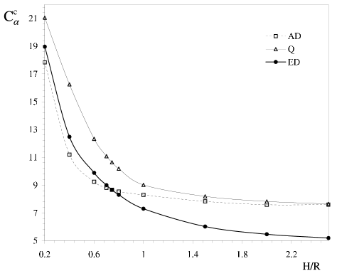
Figure 1: Critical dynamo number $C_{\alpha}^{c}$ as a function of the aspect ratio $H/R$ for a Karlsruhe-type dynamo. The two first axisymmetric ($m=0$) eigenmodes AD (axial dipole) and Q (quadrupole) are compared with the first non-axisymmetric ($m=1$) eigenmode ED (equatorial dipole).

We have found a critical aspect ratio $H/R=0.75$ which distinguishes between dominant ED and AD fields. Above this critical value ED fields are dominant while below this value AD fields are dominant. Actually, the critical aspect ratio of 0.75 is not very far from the experimental one, which is 0.83.

3.2 Ring of rolls

In the following, we investigate anisotropic $\alpha^{2}$ dynamos in an annular space defined by a gap width of $2\delta R$ with $\delta<1$. Note that in the following $R$ refers to the radius in the middle of the gap, and not to the outer radius. We consider both the $z$-independent case with $\alpha$ given by (5) and the $z$-dependent case with $\alpha$ given by (6). In each case we have considered two types of flow distinguished by the radial dependence of their vertical velocities as defined in Appendix A.2. We have called them FW1 and FW2. We computed the critical value $C_{\alpha}^{c}$ of the dynamo number $C_{\alpha}=\mu\sigma R\tilde{\alpha}$ where $\tilde{\alpha}$ stands for $\sqrt{\left\langle\alpha_{\varphi\varphi}^{2}\right\rangle}$ with $\left\langle\cdot\cdot\cdot\right\rangle$ understood as an average over $s$. According to Avalos et al. (2007) the relation between $\tilde{\alpha}$ and the real velocity of the flow is given, under the first order smoothing approximation, by $\tilde{\alpha}\approx(\eta\delta/R)R_{m\perp}R_{m\parallel}$. The quantities $R_{m\perp}=u_{0\perp}R/\eta$ and $R_{m\parallel}=u_{0\parallel}R/\eta$ are the magnetic Reynolds numbers expressed in terms of the characteristic velocities in the horizontal (i.e. perpendicular to the $z$-axis) and in the axial (i.e. parallel to the $z$-axis) direction, respectively.

3.2.1 $z$- independent case

In figure 2 the dynamo threshold is plotted in dependence on $H/R$ for both flows FW1 and FW2 for $\delta=0.5$ and $n=4$. Quite similar to the Karlsruhe dynamo case, a critical aspect ratio $H/R$ is also found here for both flows, which distinguishes between dominant ED and AD fields. Another critical value of $H/R$ is found where the second (i.e. subdominant) eigenmode is switching between AD and Q.

For a given ratio $H/R$ we found that the dynamo threshold increases monotonically when we reduced the magnitudes of $\alpha_{ss}$ and $\alpha_{\varphi\varphi}$ while keeping $\alpha_{z\varphi}$ unchanged. This is related to the impossibility of having dynamo action with a z-independent horizontal flow only.

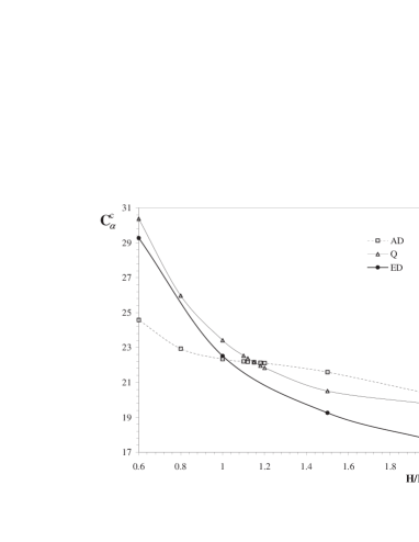
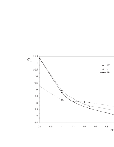
Figure 2: Critical dynamo number $C_{\alpha}^{c}$ as a function of the aspect ratio $H/R$ for an ${\alpha}$ matrix according to (5) with $\delta=0.5$. The two first axisymmetric ($m=0$) eigenmodes AD (axial dipole) and Q (quadrupole) are compared with the first non-axisymmetric ($m=1$) eigenmode ED (equatorial dipole). Plot (a) for FW1 and (b) for FW2.

In figure 3, the rescaled dynamo threshold $\delta C_{\alpha}^{c}$ is plotted in dependence on $\delta$ for both flows FW1 and FW2. We introduce here another distinction between the case of ”free rolls” (for which the number of pairs of rolls is kept equal to 4 independently of the value of $\delta$) and the case of ”compact rolls” (for which the rolls have the same extension in azimuthal and radial direction and the number of pairs of rolls scales like $n=\pi/2\delta$). In neither case was there any indication for a critical value of $\delta$ below which the dominant $m=1$ mode is clearly replaced by a dominant $m=0$ mode. However, for small values of $\delta$, the values of $\delta C_{\alpha}^{c}$ for the $m=0$ mode come very close to those of the $m=1$ mode.

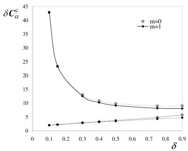
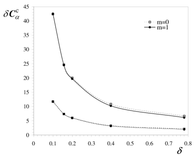
Figure 3: The rescaled dynamo threshold $\delta\,C_{\alpha}^{c}$ in dependence on $\delta$ for FW1(upper curves) and FW2(lower curves), and fix aspect ratio $H/R=2$. The dashed (solid) line corresponds to axisymmetric (non axisymmetric) fields. Plot (a) for the case of ”free rolls” and (b) for the case of ”compact rolls”.

In the case of free rolls it is remarkable that $\delta C_{\alpha}^{c}$ decreases with $\delta$ for FW1 and increases for FW2. The geometries of the magnetic field produced by FW1 and FW2 for $\delta=0.3$ have indeed different symmetries. This is illustrated in figures 4 and 5 where poloidal vectors and azimuthal contour of the magnetic field are plotted. On the other hand the symmetries are similar for $\delta=0.9$.

$\delta$	$m=0$		$m=1$
0.9
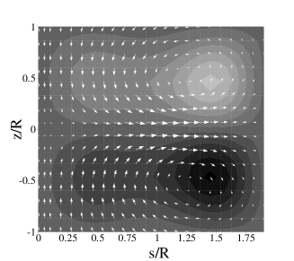
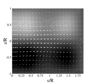
0.3

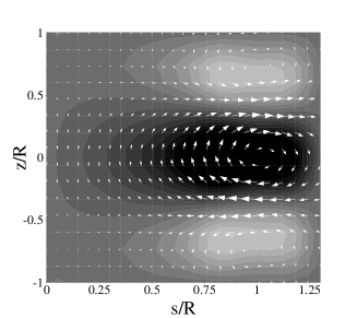
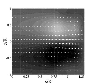
Figure 4: Poloidal field component together with contour plots of azimuthal field for FW1 with free rolls, for $\delta=0.3$, $\delta=0.9$, $m=0$, $m=1$. Ordinate axis runs from $-H/2R$ to $H/2R$, corresponding to $H/R=2$. For the non-axisymmetric case ($m=1$) the plot represents the numerical solution in the meridional plane at $\varphi=0$. However, one should notice the degeneration of the eigenvalue problem with respect to any rotation of the eigenmode in $\varphi$-direction.

$\delta$	$m=0$		$m=1$
0.9
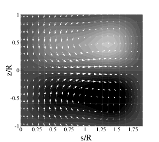
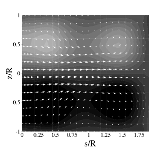
0.3

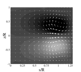
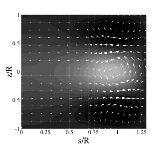
Figure 5: Same caption as figure 4 but for FW2.

3.2.2 $z$-dependent case

In figure 6, $C_{\alpha}^{c}$ is plotted in dependence on $H/R$ in the $z$ dependent case for $\delta=0.5$ and $n=4$. We find now that oscillatory non-axisymmetric fields are always the most easily excitable solutions for both flow types FW1 and FW2. However, the axisymmetric solutions are getting closer to non-axisymmetric ones as $H/R$ is reduced. For the FW1 flow a transition between steady and oscillatory magnetic fields is observed for the mode $m=0$ at a certain value $H/R\sim 1$ (the precise value could not be determined since the numerical solution of the problem is quite time consuming) . In all cases non-dipolar fields only were found.

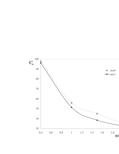
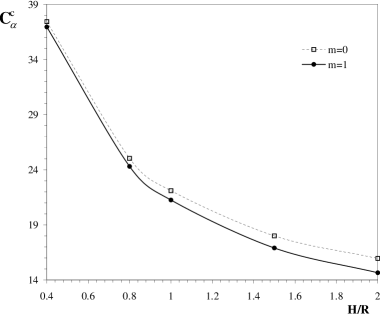
Figure 6: Critical dynamo number $C_{\alpha}^{c}$ as a function of cylinder aspect ratio $H/R$ for an $\alpha$ matrix according to (6). (a) FW1 and (b) FW2. The dashed (solid) line corresponds to axisymmetric (non axisymmetric) fields. Solutions in (a) are always oscillatory except for $m=0$ and higher values of $H=1.04$ where solutions are steady. Solutions in (b) are always oscillatory.

4 Conclusions

We have explored the influence of geometrical parameters on spatial structure and temporal variations of magnetic fields generated by kinematic anisotropic $\alpha^{2}$ dynamos working in a finite cylinder. The $\alpha$ coefficients were calculated for specific flow patterns, following the lines of mean field concept, and the corresponding dynamo solutions were calculated using the integral equation approach. The obtained results show that this kind of dynamos can switch from dominant equatorial dipoles to dominant axial dipoles just by reducing the aspect ratio of the cylinder. This transition occurs for quite different forms of $\alpha$: constant, as in the Karlsruhe dynamo experiment, or having a purely radial dependence, as the one obtained in a flow described by axially invariant helical columns. On the other hand, such a transition does not occur when the relative gap width $\delta$ is reduced (at least not for the considered aspect ratio). When $\alpha$ has an additional axial dependence, dominant dynamo solutions are only oscillatory $m=1$ modes. In addition for the $m=0$ mode both steady and oscillatory solutions were obtained.

Appendix A: Specification of the velocity field

A.1 General assumptions

We specify the motion of an incompressible conducting fluid $\mathrm{\mathbf{u}}$, so that it corresponds to a ring of columnar vortices.The ring is coated by an interval $1-\delta\leq s/R\leq 1+\delta$ with $\delta<1$. Outside this interval the fluid is assumed to be at rest. It is assumed that $\mathrm{\mathbf{u}}$ is steady, $z$-independent and varies with $\varphi$ like $\exp(\mbox{i}n\varphi)$, where $n$ is the number of vortex pairs. We use the representation

$$\mathrm{\mathbf{u}} = -\nabla\times(\mathrm{\mathbf{e}}_{z}\times\nabla\Phi)-\mathrm{\mathbf{e}}_{z}\times\nabla\Psi,$$

$$\qquad\qquad\qquad\qquad\Phi = u_{0\parallel}R^{2}\phi(s)\cos(n\varphi)\,,\quad\Psi=u_{0\perp}R\,\psi(s)\cos(n\varphi).\qquad\;\;{\rm(A.1)}$$

The two terms on the right-hand side of $\mathrm{\mathbf{u}}$ correspond to the vertical (poloidal) and horizontal (toroidal) parts of the velocity. The constant quantities $u_{0\perp}$ and $u_{0\parallel}$ define the intensity of the considered flow. We further express $\mathrm{\mathbf{u}}$ by

$$\qquad\qquad u_{s}=\hat{u}_{s}(s)\sin(n\varphi),\quad u_{\varphi}=\hat{u}_{\varphi}(s)\cos(n\varphi),\quad u_{z}=\hat{u}_{z}(s)\cos(n\varphi).\qquad\;{\rm(A.2)}$$

The connection between (A.1) and (A.2) is given by

$$\qquad\qquad\hat{u}_{s}=-u_{0\perp}R\,\frac{n}{s}\psi\,,\quad\hat{u}_{\varphi}=-u_{0\perp}R\,\frac{\partial\psi}{\partial s}\,,\quad\hat{u}_{z}=-u_{0\parallel}R^{2}D_{n}\phi\,,\qquad\qquad\,\mathrm{(A.3)}$$

where $D_{n}\phi=s^{-1}\partial_{s}(s\,\partial_{s}\,\phi)-(n/s)^{2}\phi.$

A.2 Specific examples

We consider two flows which differ only in the radial dependence of $u_{z}$. The first flow (FW1) is defined by

$$\psi=C_{\psi}\left(1-\xi^{2}\right)^{3},\quad\hat{u}_{z}/u_{0\parallel}=C_{z}\left(1-\xi^{2}\right)^{2},\quad\xi=\frac{\left(s/R\right)-1}{\delta}\,,\quad\mbox{if}\quad|\xi|<1$$

$$\phi=\psi=0\quad\mbox{otherwise}\,.\qquad\qquad\qquad\qquad\qquad\qquad\qquad\qquad\qquad\qquad\>\mathrm{(A.4)}$$

The second one (FW2) by

$$\psi=C_{\psi}\left(1-\xi^{2}\right)^{3},\quad\phi=C_{\phi}\left(1-\xi^{2}\right)^{3},\quad\xi=\frac{\left(s/R\right)-1}{\delta}\,,\quad\mbox{if}\quad|\xi|<1$$

$$\phi=\psi=0\quad\mbox{otherwise}\,.\qquad\qquad\qquad\qquad\qquad\qquad\qquad\qquad\qquad\qquad\>\mathrm{(A.5)}$$

The factors $C_{\psi}$ , $C_{\phi}$ and $C_{z}$ were chosen such that the average of $u_{z}/u_{0\parallel}$ over a surface given by $1-\delta\leq s/R\leq 1+\delta$, $-\pi/2n\leq\varphi\leq\pi/2n$ and $z/R=\mbox{constant}$ as well as the average of $u_{\varphi}/u_{0\perp}$ at $\varphi=0$ over $1\leq s/R\leq 1+\delta$ are equal to unity,

$$C_{\psi}=\delta,\quad C_{z}=\frac{{15\pi}}{16},$$

$$\quad\quad C_{\phi}=\left.{\frac{15\pi\delta^{7}}{n^{2}}}\right/\left[2\delta\left(15-40\delta^{2}+33\delta^{4}\right)+15\left(1-\delta^{2}\right)^{3}\>\log\left(\frac{1-\delta}{1+\delta}\right)\right].\qquad\;\mathrm{(A.6)}$$

The flow definitions (A.4) and (A.5) ensure that $u_{s}$, $u_{\varphi}$ and $u_{z}$ are continuous and have continuous derivatives everywhere. In figure 7 we give an example of both flow geometries.

Figure 7: Representation of a ring of rolls with four vortex pairs ($n=4$) and dimensionless annular width $\delta=0.5$. Plot (a) shows radial profile of the dimensionless vertical velocity in a vortex for first flow (FW1, dashed line) and second flow (FW2, solid line), while plot (b) shows streamlines of horizontal fluid motion for both flows. Solid and dashed lines correspond to opposite circulations.

Appendix B: Determination of $\cal{E}$

We consider an electromotive force $\cal{E}$ generated by a flow structured in helical columns between two concentric cylinders that was coined a ”ring of rolls”. Assuming that $\mathrm{\mathbf{u}}$ and $\mathrm{\mathbf{B}}$ do not depend on $z$, we look for representations of $\cal{E}$ in the general form

$$\qquad\qquad\qquad\qquad\quad{\mathcal{{E}}}_{\kappa}(s)=\int_{0}^{\infty}K_{\kappa\lambda}(s,s^{\prime})\,\overline{B}_{\lambda}(s^{\prime})\,s^{\prime}\,\mbox{d}s^{\prime}\,,\qquad\qquad\qquad\qquad\quad\>{\rm(B.1)}$$

where $\kappa$ and $\lambda$ stand for $s$, $\varphi$ or $z$. Using a Taylor expansion of $\overline{B}_{\lambda}$ , we write the last equation as

$$\qquad\qquad\qquad\qquad\quad{\mathcal{{E}}}_{\kappa}(s)=\alpha_{\kappa\lambda}(s)\,\overline{B}_{\lambda}(s)+\beta_{\kappa\lambda s}(s)\,\frac{1}{R}\frac{\partial\overline{B}_{\lambda}}{\partial s}(s)+\cdots\qquad\qquad\;\;\quad\mathrm{(B.2)}$$

with

$$\alpha_{\kappa\lambda}(s) = \int_{0}^{\infty}K_{\kappa\lambda}(s,s^{\prime})\,s^{\prime}\,\mbox{d}s^{\prime},\qquad\qquad\qquad\qquad\qquad\;\>\,\mathrm{(B.3)}$$

$$\qquad\qquad\qquad\qquad\quad\beta_{\kappa\lambda s}(s) = R\int_{0}^{\infty}K_{\kappa\lambda}(s,s^{\prime})\,(s^{\prime}-s)\,s^{\prime}\,\mbox{d}s^{\prime}.\qquad\qquad\qquad\;\;\mathrm{(B.4)}$$

The first term on the r.h.s of (B.2) represents the $\alpha$ effect, the second term represents the $\beta$ effect, which will be omitted throughout the paper. The kernel $K_{\kappa\lambda}(s,s^{\prime})$ depends only on $\mathrm{\mathbf{u}}$. Under the first order smoothing approximation (FOSA), and using a definition of mean-fields by $\varphi$ averaging, an analytical expression of $K_{\kappa\lambda}(s,s^{\prime})$ was found in Avalos et al. (2007). The results are:

$$2K_{ss}(s,s^{\prime}) = -\frac{R^{2}}{\eta}\,\left(\frac{\partial h_{n}}{\partial s^{\prime}}(s,s^{\prime})\,\hat{u}_{\varphi}(s)\,\hat{u}_{z}(s^{\prime})+\frac{\partial h_{n}}{\partial s}(s,s^{\prime})\,\hat{u}_{z}(s)\,\hat{u}_{\varphi}(s^{\prime})\right),$$

$$2K_{\varphi\varphi}(s,s^{\prime}) = \frac{R^{2}}{\eta}\,n\,\left(\frac{h_{n}(s,s^{\prime})}{s}\,\hat{u}_{z}(s)\,\hat{u}_{s}(s^{\prime})+\frac{h_{n}(s,s^{\prime})}{s^{\prime}}\,\hat{u}_{s}(s)\,\hat{u}_{z}(s^{\prime})\right),$$

$$2K_{z\varphi}(s,s^{\prime}) = -\frac{R^{2}}{\eta}\,\left(\frac{\partial h_{n}}{\partial s}(s,s^{\prime})\,\hat{u}_{s}(s)\,\hat{u}_{s}(s^{\prime})+n\frac{h_{n}(s,s^{\prime})}{s}\,\hat{u}_{\varphi}(s)\,\hat{u}_{s}(s^{\prime})\right),$$

$$\qquad\qquad\qquad\qquad\quad K_{s\varphi} = K_{\varphi s}=K_{zs}=K_{zz}=0\,.\qquad\qquad\qquad\qquad\quad\;\;\quad{\rm(B.5)}$$

The coefficients $K_{sz}$ and $K_{\varphi z}$ are not zero, but the integrals $\int_{0}^{\infty}K_{sz}(s,s^{\prime})\,s^{\prime}\,\mbox{d}s^{\prime}$ and $\int_{0}^{\infty}K_{\varphi z}(s,s^{\prime})\,s^{\prime}\,\mbox{d}s^{\prime}$ can be shown to vanish.

The Green’s function $h_{n}$ are defined by

$$h_{n}(s,s^{\prime})=\frac{1}{2n}\left(\frac{s^{\prime}}{s}\right)^{2} s^{\prime}\leq s$$ for

$$\qquad\qquad\qquad\qquad\quad h_{n}(s,s^{\prime})=\frac{1}{2n}\left(\frac{s}{s^{\prime}}\right)^{2} s\leq s^{\prime}\,.\qquad\qquad\qquad\qquad\qquad\mathrm{(B.6)}$$ for

As in Avalos et al. (2007), we can further represent

$$\alpha_{\kappa\lambda}=\frac{\eta}{R}\,R_{m\perp}\left\{\begin{array}[]{c}R_{m\perp}\\ R_{m\parallel}\end{array}\right\}\widetilde{\alpha}_{\kappa\lambda}\quad\textrm{if}\quad(\kappa\lambda)=\left\{\begin{array}[]{cc}(z\varphi)\\ (ss),&(\varphi\varphi)\end{array},\right.\;\widetilde{\alpha}_{\kappa\lambda}=0\quad\textrm{otherwise.}$$

$$\qquad\qquad\qquad\qquad\qquad\qquad\qquad\qquad\qquad\qquad\qquad\qquad\qquad\qquad\qquad\qquad\quad\,\mathrm{(B.7)}$$

where $\widetilde{\alpha}_{\kappa\lambda}$ is a dimensionless quantity independent of magnetic Reynold numbers $R_{m\perp}=u_{0\perp}R/\eta$ and $R_{m\parallel}=u_{0\parallel}R/\eta$. In figure 8, the $s/R$ profile of the three non-zero dimensionless $\widetilde{\alpha}_{\kappa\lambda}$ coefficients are represented for both flows FW1 and FW2.

Figure 8: Radial profile of the dimensionless quantity $\widetilde{\alpha}_{\kappa\lambda}$ for (a) FW1 and (b) FW2, both for $n=4$ and $\delta=0.5$.

Appendix C: Numerical approach

The correct handling of the non-local boundary conditions for the magnetic field is a notorious problem for the simulation of dynamos in non-spherical domains. Here, the kinematic eigenvalue problem in finite cylinders is solved by the integral equation approach (Stefani et al. 2000, Xu et al. 2004a, Xu et al. 2004b, Xu et al. 2006). Basically, we use the following three integral equations:

$$\mathrm{\mathbf{B}}({\mathbf{r}}) = \frac{\mu\sigma}{4\pi}\int_{V}\frac{(\alpha\circ\mathrm{\mathbf{B}}({\mathbf{r}}^{\prime}))\times{(\mathbf{r}-\mathbf{r}^{\prime})}}{|{\mathbf{r}}-{\mathbf{r}}^{\prime}|^{3}}{\rm d}V^{\prime}-\frac{\mu\sigma p}{4\pi}\int_{V}\frac{{\mathbf{A}}({\mathbf{r}}^{\prime})\times({\mathbf{r}}-{\mathbf{r}}^{\prime})}{|{\mathbf{r}}-{\mathbf{r}}^{\prime}|^{3}}{\rm d}V^{\prime}$$

$$-\frac{\mu\sigma}{4\pi}\int_{S}\phi({{\mbox{\boldmath$\zeta$}}}^{\prime})\>{\mathbf{n}}({{\mbox{\boldmath$\zeta$}}}^{\prime})\times\frac{{\mathbf{r}}-{{\mbox{\boldmath$\zeta$}}}^{\prime}}{|{\mathbf{r}}-{{\mbox{\boldmath$\zeta$}}}^{\prime}|^{3}}{\rm d}S^{\prime},\qquad\qquad\qquad\qquad\qquad\mathrm{(C.1)}$$

$$\frac{1}{2}\phi({{\mbox{\boldmath$\zeta$}}}) = \frac{1}{4\pi}\int_{V}\frac{(\alpha\circ\mathrm{\mathbf{B}}({\mathbf{r}}^{\prime}))\cdot({{\mbox{\boldmath$\zeta$}}}-{\mathbf{r}}^{\prime})}{|{{\mbox{\boldmath$\zeta$}}}-{\mathbf{r}}^{\prime}|^{3}}{\rm d}V^{\prime}-\frac{p}{4\pi}\int_{V}\frac{{\mathbf{A}}({\mathbf{r}}^{\prime})\cdot({{\mbox{\boldmath$\zeta$}}}-{\mathbf{r}}^{\prime})}{|{{\mbox{\boldmath$\zeta$}}}-{\mathbf{r}}^{\prime}|^{3}}{\rm d}V^{\prime}$$

$$-\frac{1}{4\pi}\int_{S}\phi({{\mbox{\boldmath$\zeta$}}}^{\prime})\>{\mathbf{n}}({{\mbox{\boldmath$\zeta$}}}^{\prime})\cdot\frac{{{\mbox{\boldmath$\zeta$}}}-{{\mbox{\boldmath$\zeta$}}}^{\prime}}{|{{\mbox{\boldmath$\zeta$}}}-{{\mbox{\boldmath$\zeta$}}}^{\prime}|^{3}}{\rm d}S^{\prime},\qquad\qquad\qquad\quad\;\;\quad\quad\quad\mathrm{(C.2)}$$

$$\qquad\qquad{\mathbf{A}}({\mathbf{r}}) = \frac{1}{4\pi}\int_{V}\frac{\mathrm{\mathbf{B}}({\mathbf{r}}^{\prime})\times({\mathbf{r}}-{\mathbf{r}}^{\prime})}{|{\mathbf{r}}-{\mathbf{r}}^{\prime}|^{3}}{\rm d}V^{\prime}+\frac{1}{4\pi}\int_{S}{\mathbf{n}}({{\mbox{\boldmath$\zeta$}}}^{\prime})\times\frac{\mathrm{\mathbf{B}}({{\mbox{\boldmath$\zeta$}}}^{\prime})}{|{\mathbf{r}}-{{\mbox{\boldmath$\zeta$}}}^{\prime}|}{\rm d}S^{\prime},\quad{\rm(C.3)}$$

where $\mathrm{\mathbf{B}}$ is the magnetic field, ${\mathbf{A}}$ the vector potential, $\phi$ the electric potential, ${\mathbf{n}}$ the outward directed unit vector at the boundary $S$. The complex constant $p$ contains as its real part the growth rate and as its the imaginary part the frequency of the eigenfield. The matrix $\alpha$ represents the $\alpha$-effect defined by (5) or by (6).

The reduction of the problem to cylindrical problems with azimuthal waves $\exp\left({\textrm{i}}\,m\varphi\right)$ was described in Xu et al. (2006). Finally, we end up with a generalised eigenvalue problem for the critical dynamo number $C_{\alpha}^{c}$ (in the steady case), or for the complex constant $p$ (in the unsteady case). The QR method is employed to solve this eigenvalue problem which gives also the eigenmodes of the magnetic field.

References

Aubert, J. and Wicht, J., Axial versus equatorial dipolar dynamo models with implications for planetary magnetic fields. Earth. Plan. Sci. Lett., 2004, 221, 409-419.

Avalos-Zúñiga, R., Plunian, F., and Rädler, K.-H., Rossby waves and $\alpha$-effect. 2007, to be submitted.

Busse, F.H., Model of geodynamo. Geophys. J. R. Astron. Soc., 1975, 42, 437-459.

Gailitis, A., Self-excitation conditions for a laboratory model of geomagnetic dynamo. Magnetohydrodynamics, 1967, 3, 23-29.

Giesecke, A., Rüdiger, G. and Elstner, D., Oscillating $\alpha^{2}$-dynamos and the reversal phenomenon of the global geodynamo. Astron. Nachr., 2005a, 326, 693-700.

Giesecke, A., Ziegler, U. and Rüdiger, G., Geodynamo $\alpha$-effect derived from box simulations of rotating magnetoconvection. Phys. Earth Planet. Inter., 2005b, 152, 90-102.

Grote, E. and Busse, F.H., Hemispherical dynamos generated by convection in rotating spherical shells. Phys. Rev. E, 2000, 62, 4457-4460.

Gubbins, D., Barber, C.N., Gibbons, S. and Love, J.J., Kinematic dynamo action in a sphere. II Symmetry selection. Proc. R. Soc. Lond. A, 2000, 456, 1669-1683.

Ishihara, N. and Kida, S., Dynamo mechanism in a rotating spherical shell: competition between magnetic field and convection vortices. J. Fluid Mech., 2002, 465, 1-32.

Melbourne, I., Proctor, M.R.E., & Rucklidge, A.M., A heteroclinic model of geodynamo reversals and excursions, in: Dynamo and Dynamics, a Mathematical Challenge (eds. P. Chossat, D. Armbruster and I. Oprea), Kluwer, Dordrecht, 2001, pp. 363-370.

Olson, P., Christensen, U. and Glatzmaier, G.A., Numerical modelling of the geodynamo: Mechanisms of field generation and equilibration. J. Geophys. Res., 1999, 104, 10383-10404.

Phillips, C.G., Mean dynamos, 1993, Sydney University Ph.D. Thesis

Rädler, K.-H., Some new results on the generation of magnetic fields by dynamo action. Mem. Soc. Roy. Sci. Liege, Ser. 6, 1975, VIII, 109-116.

Rädler, K.-H., Mean-Field Approach to Spherical Dynamo Models, Astron. Nachr., 1980, 301, 101-129.

Rädler, K.-H, Investigations of spherical kinematic mean-field dynamos. Astron. Nachr., 1986, 307, 89-113.

Rädler, K.-H., Apstein, E., Rheinhardt, M. and Schüler, M., The Karlsruhe dynamo experiment. A mean field approach, Stud. Geophys. Geodaet., 1998, 42, 224-231.

Rädler, K.-H.,Rheinhardt,M., Apstein, E. and Fuchs, H., On the mean-field theory of the Karlsruhe dynamo experiment. Nonlin. Proc. Geophys., 2002, 9, 171-187.

Rüdiger, G., Rapidly rotating $\alpha^{2}$-dynamos models. Astron. Nachr., 1980, 301, 181-187.

Rüdiger, G. and Elstner, D., Non-axisymmetry vs. axi-symmetry in dynamo-excited stellar magnetic fields. Astron. Astrophys., 1994, 281, 46-50.

Rüdiger, G., Elstner, D. and Ossendrijver M., Do spherical $\alpha^{2}$-dynamos oscillate? Astron. Astrophys., 2003, 406, 15-21.

Sarson, G.R . and Jones, C.A., A convection driven geodynamo reversal model. Phys. Earth Planet. Inter., 1999, 111, 3-20.

Schaeffer N. and Cardin, P., Quasi-geostrophic kinematic dynamos at low magnetic Prandtl number. Earth Planet. Sci. Lett., 2006, 245, 595-604.

Stefani, F., Gerbeth, G. and Rädler, K.-H., Steady dynamos in finite domains: an integral equation approach. Astron. Nachr., 2000, 321, 65-73.

Stefani, F. and Gerbeth, G., Asymmetry polarity reversals, bimodal field distribution, and coherence resonance in a spherically symmetric mean-field dynamo model. Phys. Rev. Lett., 2005, 94, Art. No. 184506.

Stefani, F., Gerbeth, G., Günther, U. and Xu, M., Why dynamos are prone to reversals. Earth Planet. Sci. Lett., 2006a, 143, 828-840.

Stefani, F., Gerbeth, G. and Günther, U., A paradigmatic model of Earth’s magnetic field reversals. Magnetohydrodynamics, 2006b, 42, 123-130.

Stefani, F., Xu, M., Gerbeth, G., Ravelet, F., Chiffaudel, A., Daviaud, F. and Leorat, J., Ambivalent effects of added layers on steady kinematic dynamos in cylindrical geometry: application to the VKS experiment. Eur. J. Mech. B/Fluids, 2006c, 25, 894-908.

Stieglitz R. and Müller U., Experimental demonstration of the homogeneous two-scale dynamo. Phys. Fluids, 2001, 13, 561-564.

Tilgner, A., Small scale kinematic dynamos: beyond the $\alpha$-effect, Geophys. Astrophys. Fluid Dyn., 2004, 98, 225-234.

Weisshaar, E, A numerical study of $\alpha^{2}$- dynamos with anisotropic $\alpha$-effect. Geophys. Astrophys. Fluid Dyn., 1982, 21, 285-301.

Wicht, J. and Olson, P., A detailed study of the polarity reversal mechanism in a numerical dynamo model. Geochem. Geophys. Geosys., 2004, 5, Art. No Art. No. Q03H10.

Xu, M., Stefani, F. and Gerbeth, G., The integral equation method for a steady kinematic dynamo problem. J. Comp. Phys., 2004a, 196, 102-125.

Xu, M., Stefani, F. and Gerbeth, G. Integral equation approach to time-dependent kinematic dynamos in finite domains. Phys. Rev. E, 2004b, 70, Art. No. 056305.

Xu, M., Stefani, F. and Gerbeth, G., The integral equation approach to kinematic dynamo theory and its application to dynamo experiments in cylindrical geometry. in: Proceedings of ECCOMAS CFD 2006, (eds: P. Wesseling, E. Onate, J. Periaux), TU Delft, paper 497 (CD).

Yoshimura, H., Wang, Z. and Wu, F., Linear astrophysical dynamos in rotating spheres: mode transition between steady and oscillatory dynamos as a function of dynamo strength and anisotropic turbulent diffusivity. Astrophys. J., 1984, 283, 870-878.