Eulerian and Lagrangian Statistics from high resolution Numerical Simulations of weakly compressible turbulence

Abstract

We report a detailed study of Eulerian and Lagrangian statistics from high resolution Direct Numerical Simulations of isotropic weakly compressible turbulence. Reynolds number at the Taylor microscale is estimated to be around $600$. Eulerian and Lagrangian statistics is evaluated over a huge data set, made by $1856^{3}$ spatial collocation points and by 16 million particles, followed for about one large-scale eddy turn over time. We present data for Eulerian and Lagrangian Structure functions up to ten order. We analyse the local scaling properties in the inertial range and in the viscous range. Eulerian results show a good superposition with previous data. Lagrangian statistics is different from existing experimental and numerical results, for moments of sixth order and higher. We interpret this in terms of a possible contamination from viscous scale affecting the estimate of the scaling properties in previous studies. We show that a simple bridge relation based on Multifractal theory is able to connect scaling properties of both Eulerian and Lagrangian observables, provided that the small differences between intermittency of transverse and longitudinal Eulerian structure functions are properly considered.

1 Introduction

In the last few years many interesting and remarkabe results have been obtained by investigating the statistical properties of Lagrangian particles advected by a turbulent flow –for a recent review see Toschi & Bodenschatz (2009). For Lagrangian particles we mean simple point like ideal tracers, whose instantaneous velocity coincides with the local Eulerian velocity field, ${\bf u}({\bf x},t)$: $\dot{\bf X}(t)={\bf u}({\bf X}(t),t)$. Beside being relevant in many applications, where transport and/or aggregation of particles is important, the study of fully developed turbulence in the Lagrangian framework has opened important new directions of scientific investigations. In particular, small scale intermittency of turbulent flows and dissipation range can be probed more efficiently in the Lagrangian framework as shown experimentally since the works of La Porta et al. (2001); Mordant et al. (2001, 2006); Ott & Mann (2000); Berg et al. (2006); Bourgoin et al. (2006); Luthi et al. (2005); Berg et al. (2009) and numerically in Biferale et al. (2005); Yeung et al. (2006); Homann et al. (2007); Mordant et al. (2006), (see also Biferale et al. (2008) and Arneodo et al. (2008) for comparison between experimental and numerical Lagrangian data). Moreover, Lagrangian and Eulerian measurement (those on the reference frame of the laboratory) should be intimately statistically connected as pointed out for the first time in Borgas (2003); Boffetta et al. (2002), the hope is to learn about the former from the study of the latter and viceversa.

In this paper we present some new results concerning the statistical properties of the Lagrangian and Eulerian velocity field in weakly compressible turbulent flow. The flow is the outcome of a high resolution numerical simulations described in the next section. Our motivation is threefold: due to the high spatial resolution and the huge particle statistics (16 millions of particles) we are able to extract the statistics of the Lagrangian velocity field with high accuracy and relatively small error bars. From this point of view we are able to assess, for the first time at this Reynolds numbers, statistical fluctuations in the Lagrangian domain as intense as those given by moments up to order 10. The second purpose is to understand whether the effect of the weak compressibility changes the statistical properties of Eulerian and Lagrangian velocity field with respect to previous numerical investigations of incompressible isotropic turbulent flows. Preliminary results concerning this point have been already published in Benzi et al. (2008); here a more detailed analysis on new observables is reported. In particular, we are interested in understanding the effect of intermittency in the inertial range for Lagrangian particles. Some results concerning dissipative scales will be also presented. Finally, our third motivation concerns with the statistical link between Lagrangian and Eulerian measurements. Concerning this point we show that a simple model, based on the multifractal theory, is able to translate between the two ensembles with a quantitative agreement extending over three decades from inside dissipative scales to the integral scale (Arneodo et al. (2008)).

Our main tool is the numerical computation of velocity increments over a time lag $\tau$, the so-called Lagrangian structure functions:

$${\cal S}_{i}^{(p)}(\tau)=\langle[v_{i}(t+\tau)-v_{i}(t)]^{p}\rangle=\langle(\delta_{\tau}v_{i})^{p}\rangle,$$ (1)

where $i=x,y,z$ are the three velocity components along a particle trajectory, $v_{i}(t)=u_{i}({{\bf x}}(t),t)$ and the average is defined over the ensemble of particle trajectories. As stationary and homogeneity is assumed, moments of velocity increments only depend on the time lag $\tau$. When isotropy is also valid, all components must be symmetric and we will drop the dependency on the spatial index. In the inertial range, for time lags smaller than the integral time and larger than the Kolmogorov time, $\tau_{\eta}\ll\tau\ll T_{L}$, non-linear energy transfer governs the dynamics. From a dimensional viewpoint, only the scale $\tau$ and the energy transfer $\epsilon$ should enter the structure functions. The only admissible choice in isotropic statistics is ${\cal S}^{(p)}(\tau)\sim(\epsilon\tau)^{p/2}$, but it does not take into account the fluctuating nature of dissipation. Many empirical studies (Toschi & Bodenschatz (2009)) have indeed shown that the tail of the probability density functions of $\delta_{\tau}v$ become increasingly non-Gaussian at decreasing $\tau/T_{L}$, leading to intermittency and to anomalous scaling exponents, meaning a breakdown of the dimensional law, i.e.

$${\cal S}^{(p)}(\tau)\sim\tau^{\xi^{(p)}}\,$$ (2)

with $\xi^{(p)}\neq p/2$.

As we will review and test in details later, the Lagrangian measurements can be linked to Eulerian Structure Function (ESF). In isotropic statistics we may have two different Eulerian increments, longitudinal and transverse (see Frisch (1995) for a textbook introduction to scaling in homogeneous and isotropic turbulence):

$$\begin{cases}S^{(p)}_{L}(r)\equiv\langle[{\bf u}({\bf x}+{\bf r})-{\bf u}({\bf x})]\cdot{\hat{\bf r}}]^{p}\rangle\\ S^{(p)}_{T}(r)\equiv\langle|{\bf u}({\bf x}+{{\bf r}}_{T})-{\bf u}({\bf x})|^{p}\rangle,\qquad{{\bf r}}_{T}\cdot{{\bf u}}=0.\end{cases}$$ (3)

It is well established, (Arneodo et al. (1996); Frisch (1995)) that also Eulerian statistics have anomalous scaling, for $\eta\ll r\ll L$:

$$\begin{cases}S^{(p)}_{L}(r)\sim r^{\zeta_{L}^{(p)}}\\ S^{(p)}_{T}(r)\sim r^{\zeta_{T}^{(p)}}.\\ \end{cases}$$ (4)

From a theoretical point of view, in isotropic turbulence one would expect that longitudinal and transverse fluctuations have the same scaling, $\zeta_{L}^{(p)}=\zeta_{T}^{(p)}$ (see Biferale & Procaccia (2005) for a review on anisotropic turbulence). This is not what was observed in many experimental and numerical analysis (Boratav & Pelz (1997); van der Water (1999); Shen & Warhaft (2002); Chen et al. (1997); Zhou & Antonia (2000); Dhruva et al. (1997)). Discrepancy can be due to finite Reynolds numbers (Hill (2001); He et al. (1998)) or to some remnant small-scale anisotropy (Biferale & Procaccia (2005)). Still, even large Reynolds number DNS with isotropic forcing show some persistent differences between $\zeta_{L}^{(p)}$ and $\zeta_{T}^{(p)}$ as shown in Ishihara et al. (2009); Gotoh et al. (2002); the same discrepancy is quantitatively confirmed in the analysis here reported. Whether this effect will persist at higher Reynolds number remains an important open question for further experimental and numerical investigations.

Recently, it has been argued that there must exists a relation between Lagrangian and Eulerian exponents, on the basis of a common multifractal description (Boffetta et al. (2002); Biferale et al. (2005)). This relation between Lagrangian and Eulerian statistical properties is highly non trivial and it is worth to understand how accurately can be verified in the existing DNS and laboratory experiments. It has been proved to be very efficient to predict the pdf of Lagrangian acceleration (Biferale et al. (2004)) and of Lagrangian Structure Functions of low order (Arneodo et al. (2008)).

The paper is organized as follows. In section (2) we discuss the numerical simulations and the data set. In section (3) we discuss the computation of the Eulerian structure functions. In section (4) we report the analysis of Lagrangian structure functions and we discuss the physical results obtained by our analysis. In section (5) we provide a theoretical interpretation of our findings by employing the multifractal framework. Conclusions follows in section (6).

2 Data set and numerical simulations

As briefly highlight in the introduction, our main purpose is to investigate intermittency of the Lagrangian/Eulerian velocity field in the inertial range for a weakly compressible isotropic turbulent flow (see figure (1) for a colorful rendering). The numerical simulation have been performed using the FLASH code developed by the Flash Center at the University of Chicago (Fisher et al. (2007)). The equation of motion are:

$$\begin{cases}{\partial_{t}\rho}+{\bm{\nabla}}\cdot({\bf u}\rho)=0\\ {\partial_{t}(\rho{\bf u})}+{\bm{\nabla}}\cdot({\bf u}{\bf u}\rho)=-{\bm{\nabla}}P+{\bm{F}}\\ {\partial_{t}(\rho E)}+{\bm{\nabla}}\cdot[{\bf u}(\rho E+P)]=0\\ P=(\gamma-1)\rho U\\ E=\rho(U+\frac{1}{2}u^{2})\end{cases}$$ (5)

where $\rho$ is the mass density, ${\bf u}$ the velocity, $P$ the pressure, $E$ the total energy density, $U$ the specific internal energy, and $\gamma$ is the ratio of the specific heats in the system. Finally, the fourth equation in (5) is the equation of state for our system. The effect of the large scale forcing ${\bm{F}}$ gives rise to a turbulent flow whose energy is transferred from scale $L_{0}$ towards small scales. The energy input $\int d^{3}x\,{\bf u}\cdot{\bm{F}}$ produces an increase of the internal energy $U$, which grows in time. One can easily show that the quantity $\int dx^{3}P\,\partial_{i}v_{i}$ represents the energy transfer from kinetic to internal energy of the flow. The sound speed increases in time as well, while the average Mach number is order $0.3$. The numerical simulation is done for isotropic and homogeneous forcing with a resolution $1856^{3}$. The integration in time have been done for three eddy turnover times after a transient evolution. More details on the numerical code can be found in Benzi et al. (2008). The code develops density gradients due to compressibility. Despite compressible effects, which lead to highly non-trivial scaling of density and entropy fluctuations (Benzi et al. (2008); Porter et al. (2002)), the net feedback on the velocity scaling is very weak, if any. Here we show that to the best of our testing ability, velocity fluctuations in the inertial range are indistinguishable from those measured on incompressible fluid turbulence.
Although the integration is formally inviscid, there is a net energy transfer from the turbulent kinetic energy $1/2\rho u^{2}$ to the internal energy. Thus we may think that an effective viscosity $\nu_{\mbox{eff}}$ is acting on the system. In order to estimate it, we proceed as if the Kolmogorov 4/5 equation (see Frisch (1995)), valid for incompressible turbulence applies to our case –with effective parameters:

$$S_{L}^{(3)}(r)=-\frac{4}{5}\epsilon_{\mbox{eff}}r+6\nu_{\mbox{eff}}\frac{d}{dr}S_{L}^{(2)}(r).$$ (6)

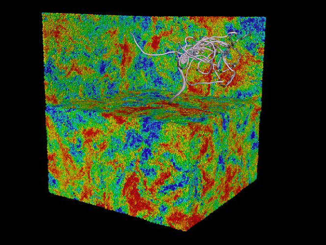
Figure 1: Example of Eulerian and Lagrangian rendering. Both the intensity of the Eulerian velocity field at a given time and the Lagrangian evolution of a bunch of particles with trajectories ending at the time of the Eulerian snapshot are shown. Notice that the Lagrangian particles have an initial smooth evolution because we also show the initial transient time when the underlying Eulerian field was chosen smooth and with low energy. The bunch of particles was chosen such has to encounter a vortex filaments during their evolution. Figure courtesy of B. Gallagher.

A fit of our data with this formula gives, $\epsilon_{\mbox{eff}}=0.054,\nu_{\mbox{eff}}=8.3\cdot 10^{-6}$, which corresponds to a Kolmogorov scale, $\eta=(\nu_{\mbox{eff}}^{3}/\epsilon_{\mbox{eff}}^{1/4})$, equivalent to roughly half grid cell and to $R_{\lambda}\sim 600$. The dynamical effects of the effective viscosity is however different from what one usually observes in the Navier Stokes equations, i.e. the dissipation range does not behave similarly to the Navier Stokes solutions. Thus, while on the energy flux (i.e. the third order structure functions) we still observe an effective dissipation, the dissipation range is changed according to the specific mechanism employed in the simulation, namely the increase of internal energy and the artificial numerical viscosity added up to smooth too high gradients (Fisher et al. (2007)).

Figure 2: Left: Test of the isotropic and incompressible constraint, we show the LHS and the RHS of (7). In the inset we have a percentage estimate of the breaking of the relation: (RHS-LHS)/LHS. Notice that percentage-wise the relation is well verified, within $5\%$ of accuracy. Right: third order longitudinal structure functions, $S_{L}^{(3)}(r)$ with the power law exact relation coming from the $4/5$ law (Frisch (1995)). Inset: compensated plot, $S_{L}^{(3)}(r)/r$.

Let us quantify the importance of the small compressibility on the statistics of the velocity field. For isotropic and incompressible fields, there exists an exact relation which connects second order longitudinal and transverse structure functions (Frisch (1995)):

$$S^{(2)}_{T}(r)=S^{(2)}_{L}(r)+\frac{r}{2}\frac{d}{dr}S^{(2)}_{L}(r),$$ (7)

this equation is useful because any deviations from it gives a quantitative hint on the cumulative importance of anisotropy and compressibility, scale-by-scale. We show in the left panel of Fig. (2) the comparison between $S^{(2)}_{T}(r)$ and its reconstruction via the RHS of (7). As one can see the agreement is good. Combined effects due to anisotropy and compressibility are less than a few percent for second-order statistics (see also Fig.3 for higher-order statistics).

3 Intermittency and anomalous scaling in the Eulerian velocity field

We start our analysis by measuring the scaling behavior of the Eulerian structure functions. In the right panel of Fig. (2) we show the third order longitudinal ESF as measured in our DNS. As one can see, in log-log plot there is a clean scaling range over more than one decade extending from $r/\eta\in[10:100]$, with a slope close to the scaling prediction, $S_{L}^{(3)}(r)\sim r$. In Fig. (3) we show a typical log-log plot of Longitudinal ESF for $p=2,6,10$. Again, a qualitative scaling behaviour is clearly detectable. The high resolution and the highly isotropic forcing used in our DNS, allows also for a precise quantitative assessment of the importance of statistical and anisotropy effects on the averaged quantified. In the right panel of the same figure, we show the estimate of the statistical fluctuations (top panel) by plotting the ration between two Structure functions averaged either over the whole statistics or over one half of it. As one can see, statistical fluctuations become at maximum of order $10-20\%$ at small scales (where intermittency is more severe) and only for high order moments $p=6$ and larger. Inside the inertial range, $r>10\eta$, they are order $5\%$ or even less. Similarly, in the bottom panel we give a quantitative estimate of anisotropic residual effects, by plotting the ratio between longitudinal measurements over two different orthogonal directions. Here, as expected, deviations are larger close to the integral scale, reaching a maximum of $10\%$ for high order moments. As a result, the combined effect of statistical and anisotropic fluctuations for the Eulerian scaling are small and they result in an estimate of the error bars that is within the size of the symbols for the log-log plot showed on the left panel of Fig. (3).

One of the pluses of high resolution DNS is the possibility to go beyond log-log plot, analysing scaling properties locally, with high precision. In order to do that, we analyse scaling by using the magnifying glass of local scaling exponent, (LSE), given by the log-derivative of Structure Functions:

$$\zeta_{L}^{(p)}(r)\equiv\frac{d\log S_{L}^{(p)}(r)}{d\log r};\qquad\zeta_{T}^{(P)}(r)\equiv\frac{d\log S_{T}^{(p)}(r)}{d\log r}.$$ (8)

The advantage to rely on LSE is twofold. First, it allows for assessing statistical properties locally, removing large-order non-universal contributions coming from the overall prefactors in the SF. Second, and more importantly, they assess scaling without the need for any fitting; in other words, they are just the outcome of a measure and they do not depend on an arbitrary definition as the extension of the inertial range, in order to define the degree of intermittency. For instance, let us consider, the scaling of fourth order longitudinal Flatness. It is easy to see that it can be rewritten, independently on any scaling assumption and for all separations $r$, as:

$$F_{L}^{(4)}(r)=\frac{S_{L}^{(4)}(r)}{(S_{L}^{(2)}(r))^{2}}=(S_{L}^{(2)}(r))^{\phi_{L}^{(4)}(r)};\qquad\phi_{L}^{(4)}(r)=\frac{\zeta_{L}^{(4)}(r)}{\zeta_{L}^{(2)}(r)}-2.$$ (9)

In other words, the presence of intermittency, i.e. a non trivial scale-dependent Flatness behaviour, is directly measure by how much the ratio of LSE, $\zeta_{L}^{(4)}(r)/\zeta_{L}^{(2)}(r)$ is different from its dimensional value, $2$, scale-by-scale.

Figure 3: Left: log-log plot of Longitudinal Eulerian Structure Functions, $S_{L}^{(p)}(r)$ for $p=2,6,10$. Right: estimate of the anisotropic fluctuations, $\langle[u_{x}({\bf x}+r_{x})-u_{x}({\bf x})]^{p}\rangle/\langle[u_{y}({\bf x}+r_{y})-u_{y}({\bf x})]^{p}\rangle$, for $p=2,6,10$ (bottom). Estimate of the statistical fluctuations, obtained by plotting the ratio of $S_{L}^{(p)}(r)$ calculated over the whole statistics or over one half of it (top). The sum of the two error sources leads to error bars that are of the order of the symbol size on the left panel.

Let us start to analyze the LSE for the Longitudinal and Transverse ESF. In figure (4) we show the LSE for $p=2,4,6,8$ and in figure (5) we show the LSE for $p=10$. Let us first notice that Longitudinal and Transverse statistics have significantly different viscous cut-off, with transverse fluctuations having the tendency to have less important viscous damping with respect to the longitudinal one (Gotoh et al. (2002)). This is an effect already present for low order $p=2$ (bottom left panel) and therefore certainly induced, at least partially, by geometrical constraints as the ones discussed about eqn. (7). Beside this remark, let us also notice the small –in amplitude– but important –in principle– difference in the scaling exponents form longitudinal and transverse. Up to $p=4$ the LSE are almost coinciding, within error bars, in the range of scales $r/\eta\in[20:80]$. For larger orders, we start to detect a difference, with the transverse being systematically below the longitudinal. This difference becomes significantly visible for $p=10$ as shown separately in Fig. (5). Note that this statements is not the outcome of any fitting procedure and what is shown in figure (4) and (5) is a measurements independent on any theoretical interpretation.

Figure 4: Local scaling exponents, $\zeta_{L}^{(p)}(r),\zeta_{T}^{(p)}(r)$ of Eulerian Lagrangian and Transverse structure functions for $p=2,4,6,8$. Error bars are obtained by estimating the residual anisotropy, and they are given by the spread between measurements on different directions, ${\bf r}/r=\hat{x},\hat{y},\hat{z}$. Statistical error bars are smaller. The horizontal straight line corresponds to the k41 dimensional prediction, $\zeta^{(p)}=p/3$.

To decide about the existence –and extension– of a power-law scaling range needs some fitting. The value of the global scaling exponent, $\zeta_{L}^{(p)},\zeta_{T}^{(p)}$ would then be given by the average of the LSE in the region where they are close to constant. An error bar on the mean value can be then estimated on the basis of the oscillation induced by statistical and anisotropic effects in the fitting range and by the change as a function of the extension of the scaling range used to make the fit. Such a fitting procedure (details in the caption) leads to the summary for the global Eulerian scaling exponents depicted in the right panel of Fig. (5) and summarized also in table 1, where we compare our results also with other DNS obtained with fully incompressible Navier-Stokes equations at comparable Reynolds numbers. From a theoretical point of view, we know that there are exact constraints that fix $\zeta_{L}^{(p)}=\zeta_{T}^{(p)}$ for $p=2$ (for $p=3$ a similar constraint fix the scaling of third order longitudinal with mixed second order transverse and first order longitudinal averages). Nevertheless, there is not any strong theoretical argument suggesting the possibility that for $p\geq 4$ one should expect different scaling. So, the result shown in Figs. (4-5) is not fully understood. Whether the difference between longitudinal and transverse ESF will shrink going to higher Reynolds number remains to be investigated, and it is an important open question. The good news is that the value found in our numeric are in perfect agreement with previous results (see table 1), making us confident that they are robust and not dependent on compressibility. Even the relative scaling behaviour, obtained by plotting each structure functions versus the third order one, a procedure known as Extended Self Similarity (ESS) in the literature (Benzi et al. (1993, 1996)) does not change much the above picture. In table 1 we give also the results of the LSE for both Longitudinal and Transverse ESF estimated by using ESS. Again a small spread between longitudinal and transverse is measured. Nevertheless, it is interesting to notice that while the ESS procedure applied to longitudinal statistics reduces considerably the error bars with respect the usual LSE, for the transverse one there is not a clear gain in adopting ESS. This may suggest the possibility that the different scaling behaviour detected between, $S_{L}^{(p)}(r)$ and $S_{T}^{(p)}(r)$ maybe due to different sub-leading corrections to the main leading scaling, contributing more to the transverse scaling than to the longitudinal. Due to the lack of any hints on the possible sub-leading correction we refrain here from entering in to a fitting procedure with too many free parameters. The issue whether the different in the LSE shown in Fig. (4) is the signature of a true mismatch between the scaling properties of longitudinal and transverse fluctuations or the result of a superposition of leading and sub-leading power laws with coinciding exponents between longitudinal and transverse but with different prefactors, remains open.

Figure 5: Left: longitudinal and transverse local scaling exponents, the same of fig. (4) but for $p=10$. Right: summary of the Eulerian scaling from table 1. The two solid lines represent a fit to the scaling exponents with two different Multi Fractal spectrum $D_{L}(h)$ and $D_{T}(h)$ both having a log-Poisson statistics, (She & Leveque (1994); Dubrulle (1994)): $D_{L,T}(h)=\frac{3(h-h^{*})}{\log(\beta_{L,T})}\left[\log\left(\frac{3(h^{*}-h)}{d_{L,T}^{*}\log(\beta_{L,T})}\right)-1\right]+3-d_{L,T}^{*}$. The free parameters are chosen such as to minimize the fitting differences between Longitudinal and Transverse. The only parameter we changed is the intermittent factor $\beta_{L}=0.6$ and $\beta_{T}=0.4$ while we kept the highest singularity to be the same for the two cases, $h^{*}=1/9$. The fractal dimension of the $h^{*}$ is then fixed by the requirement that $\zeta_{L}^{(3)}=\zeta_{T}^{(3)}=1$ and must be chosen $d^{*}_{L,T}=(1-3h^{*})/(1-\beta_{L,T})$. Another alternative approach for the fit would be to fix $\beta$ and change the value of the highest singularity between longitudinal and transverse fluctuations.

p	$\zeta_{L}^{(p)}$	$\zeta_{T}^{(p)}$	$\zeta_{L}^{(p)}$ [G02]	$\zeta_{T}^{(p)}$ [G02]	$\zeta_{L}^{(p)}/\zeta_{L}^{(3)}$	$\zeta_{T}^{(p)}/\zeta_{T}^{(3)}$
2	0.71 $\pm$ 0.02	0.71 $\pm$ 0.02	0.70 $\pm$ 0.01	0.71 $\pm$ 0.01	0.69 $\pm$ 0.005	0.71 $\pm$ 0.01
4	1.29 $\pm$ 0.03	1.27 $\pm$ 0.05	1.29 $\pm$ 0.03	1.26 $\pm$ 0.02	1.28 $\pm$ 0.01	1.26 $\pm$ 0.01
6	1.78 $\pm$ 0.04	1.68 $\pm$ 0.06	1.77 $\pm$ 0.04	1.67 $\pm$ 0.04	1.75 $\pm$ 0.01	1.68 $\pm$ 0.03
8	2.18 $\pm$ 0.05	1.92 $\pm$ 0.10	2.17 $\pm$ 0.07	1.93 $\pm$ 0.09	2.17 $\pm$0.03	1.98 $\pm$ 0.1
10	2.50 $\pm$ 0.06	2.10 $\pm$ 0.20	2.53 $\pm$ 0.09	2.08 $\pm$ 0.18	2.5 $\pm$ 0.05	2.25 $\pm$ 0.15

Table 1: Estimate of the global scaling exponents, out of the figures for the local scaling exponents (4-5). The first and second columns refer to our DNS, the third and fourth to the data published in (Gotoh et al. (2002)) from a DNS at comparable Reynolds number. The last two columns correspond to the ESS estimate of our data, using the third order longitudinal ESF as a reference for the scaling of $S_{L}^{(p)}$ and using the third order transverse ESF for the scaling of $S_{T}^{(p)}(r)$. Error bars are obtained by summing the uncertainty obtained from estimating the scaling in three different spatial direction (anisotropy contributions) and by changing the scaling range in the interval $r\in[10:100]\eta$, where the global exponent is evaluated.

4 Intemittency and anomalous scaling in the Lagrangian velocity field

We now turn our attention to Lagrangian particles. As it is known, LSF shows very strong intermittency. In figure (6), we show the probability density function of $\delta_{\tau}v_{i}$, for different values of $\tau$ and averaging over the different velocity components: for small $\tau$ the probability density exhibits stretched exponential tails, as also measured experimentally in (Mordant et al. (2001)). The huge statistics at our hands, up to 16 millions trajectories of length up to one large scale eddy turn over time, $T_{L}$, allows for detecting fluctuations up to $40$ standard deviations, for the highest frequency. Concerning the LSF, we show in the same figure (right panel) a first overview on a log-log scale for moments up to $p=8$. From this panel we can already extract some conclusions. First, scaling in Lagrangian framework is not as good as the Eulerian one, as one can judge by the naked eye. This is a common feature of all Lagrangian statistics, and was already observed in many other experimental and numerical previous works.

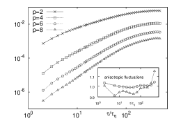
Figure 6: Left: Lagrangian PDF for a single component velocity increments along particle trajectories, over different time increments, $\tau\in[2:400]\tau_{\eta}$. Right: log-log plot of LSF for $p=2,4,6,8$. Inset: estimate of the anisotropic statistical degree: ratio between two different components of LSF, $\langle(\delta_{\tau}v_{x})^{p}\rangle/\langle(\delta_{\tau}v_{y})^{p}\rangle$, for $p=4$ (circles) and $p=8$ (triangles)

The simplest explanation is that the finite Reynolds effects are more important in Lagrangian domain: dimensional estimate gives for the Lagrangian inertial range extension the scaling $T_{L}/\tau_{\eta}\sim R_{\lambda}^{1/2}$, while in the Eulerian case we have $L/\eta\sim R_{\lambda}^{3/4}$. In the inset of the same figure, we show the importance of anisotropic fluctuations, by comparing the ration between two LSF on two different components, ${\cal S}^{(p)}_{x}(\tau)/{\cal S}^{(p)}_{y}(\tau)$ for $p=4,8$. As one can see, the importance of anisotropic fluctuations is again of the order of $10\%$ at most, for the highest moments. Such correction are of the order of the symbol size of the LSF averaged over the three components shown in the left panel. The poorer scaling in the Lagrangian domain, does not allow for a systematic assessment on the local scaling exponents as done for the Eulerian field. Here, if one wishes to retain good local properties, it is necessary to resort to the ESS method, plotting the local scaling exponents relative to one moment versus a reference one (here taken the second order):

$$\chi^{(p)}(\tau)\equiv\frac{d\log{\cal S}^{(p)}(\tau)}{d\log{\cal S}^{(2)}(\tau)},$$ (10)

which are related, in presence of pure power law scaling, to the scaling exponents of the LSF defined from (2) by the obvious relation:

$$\chi^{(p)}(\tau)\sim const.=\xi^{(p)}/\xi^{(2)}.$$ (11)

Let us stress nevertheless, that the importance of the local exponents (10) goes much beyond their interpretation as a simple proxy of the ratio between the structure functions exponents (11). Indeed, they give a clear and simple way to assess the importance of intermittency in the Lagrangian domain being the only quantities entering in the scaling properties of Lagrangian hyper-Flatness:

$${\cal F}^{(p)}(\tau)=\frac{{\cal S}^{(2p)}(\tau)}{({\cal S}^{(2)}(\tau))^{2}}=({\cal S}^{(2)}(\tau))^{\chi^{(2p)}(\tau)-p/2}.$$ (12)

Again here the same comment made for the Eulerian case is in order: via the Lagrangian hyper-Flatness (12) we are able to assess intermittency in a quantitative way, free of any fitting ambiguity, without having to assume power law properties, by simply checking the difference between $\chi^{(2p)}(\tau)$ and $p/2$, scale-by-scale.

Figure 7: Lagrangian Local scaling exponents for hyper-Flatness, $\chi^{(p)}(\tau)$, for $p=4,6,8,10$. Notice the extremely good scaling behaviour for low moments, which deteriorates only mildly for $p=6,8$. Notice also the dip region close to the viscous time scales, an effect interpreted in terms of trapping into vortex filaments (Jimenez et al. (1993); Bec et al. (2006)). The horizontal straight lines correspond to the dimensional scaling $\chi^{(p)}=p/2$.

$\chi^{(p)}$	$p=4$	$p=6$	$p=8$	$p=10$
our DNS ($R_{\lambda}\sim 600$)	1.66 $\pm$ 0.02	2.10 $\pm$ 0.10	2.33 $\pm$ 0.17	2.45 $\pm$ 0.35
EXP1 ($R_{\lambda}\sim 800$)	1.47 $\pm$ 0.18	1.73 $\pm$ 0.25	1.92 $\pm$ 0.32	1.98 $\pm$ 0.38
EXP2 ($R_{\lambda}\in[500:1000]$)	1.56 $\pm$ 0.06	1.80 $\pm$ 0.20	–	–
DNS1 ($R_{\lambda}\sim 320$)	1.51 $\pm$ 0.04	1.76 $\pm$ 0.11	–	–
DNS2 ($R_{\lambda}\sim 75$)	1.56 $\pm$ 0.03	1.82 $\pm$ 0.08	1.92 $\pm$ 0.14	1.93 $\pm$ 0.3

Table 2: First raw: summary of the local scaling exponents for Lagrangian statistics as extracted from our data shown in Fig. (7). Error bars are evaluated out of the anisotropic statistical degree, estimating the LSE out of the three different velocity components and by changing the fit range in the interval $\tau\in[20:200]$. The other rows correspond to other data available for high order moments from both experiments at comparable Reynolds numbers and numerical works at smaller Reynolds numbers. EXP1 (Xu et al. (2006)); EXP2 (Mordant et al. (2006)); DNS1 (Homann et al. (2007)); DNS2 (Mordant et al. (2006)). Notice how some of the previous data slightly underestimate the value of the scaling exponents for $p=6,8,10$. This is due to the fact that, due to the limitations either in the statistics or in the Reynolds number, it was not possible to assess scaling properties scale-by-scale as done here. For example, the fit leading to the numbers in Xu et al. (2006) and in Homann et al. (2007) (second and fourth raw) was done in the range $\tau\in[3:6]\tau_{\eta}$, well inside the dip region. Similarly, the Reyolds number of the numerical data in (Mordant et al. (2006)) (fifth row) is very low, probably the strong saturation in the values for $p=6,8,10$ reported there is due again to the presence of the dip region spoiling the scaling in the short inertial range present at $R_{\lambda}\sim 75$.

In Fig. (7) we show the hyper-Flatness local exponents for $p=4,6,8,10$. The scaling range now is good, for $\tau/\tau_{\eta}\in[20:200]$. As one can see, there are two remarkable facts. First, Lagrangian scaling is much more intermittent then the Eulerian one, if measured as a deviations from the dimensional scaling, $\chi(p)=p/2$. For example, for $p=10$, we measure $\chi^{(10)}=2.45\pm 0.35$ which is $50\%$ off from the dimensional value $\chi^{(10)}=5$. The second fact is the strong dip measured across the viscous scale, for time lags $\tau/\tau_{\eta}\in[1:10]$. This is similar to the Eulerial “bottleneck” (Lohse (1994)), while for Lagrangian structure functions was observed first in (Mazzitelli & Lohse (2004)) and interpreted as induced by the presence of small scale vortex filaments in Biferale et al. (2005); Bec et al. (2006). The value of the Lagrangian exponents measured in our DNS ar reported in table (2) and compared with previous measurements on other DNS or experiments. Let us stress that there are not other measurements with comparable statistics and Reynolds number,as the one here presented for high order moments. A global fit in log-log of the scaling properties does not allow to disentangle the inertial range from viscous-inertial contribution (affected by the dip) as they emerge from fig. (7). This explain the slightly systematic underestimate of the scaling exponents from all the previous studies with respect to our measurements. The only data presented previously for $p=8,10$ at comparable Reynolds are those published in (Xu et al. (2006)) where the scaling properties where estimated very close, if not inside, the dip region, $\tau\in[3:6]\tau_{\eta}$. Similarly was done for the data in Homann et al. (2007). The numerical data for $p=8,10$ presented in (Mordant et al. (2006)) are also understimating the value of the scaling properties with respect to our data. Probably, in this case, the very low value of the Reynolds number ($R_{\lambda}\sim 75$) is such that the whole scaling region is dominated by the viscous dip. Considering all these pitfalls, we may conclude that when scaling properties are analysed in the correct range and where statistical fluctuations are not too high, there exists a good universality in Lagrangian statistics, as also tested quantitatively for $p=4,6$ in Biferale et al. (2008); Arneodo et al. (2008). As for universality of high order moments, from $p=8$ and up, we need to wait for other data with statistical properties and Reynolds number comparable with those of this study, to decide.

5 Multifractal: a link between Eulerian and Lagrangian statistics

Multifractals have been introduce 25 years ago to explain deviations to the K41 scaling for Eulerian isotropic turbulent fluctuations (Parisi & Frisch (1985), see also Boffetta et al. (2008) for a recent review). Since those works, they have been extended to describe also velocity gradients (Nelkin (1990); Benzi et al. (1991)); multi-scale velocity correlations (Belinicher et al. (1998); Benzi et al. (1998)) and fluctuations of the Kolmogorov viscous scale (Paladin & Vulpiani (1987); Meneveau (1996); Biferale (2008); Frisch & Vergassola (1991)). Let us notice that other attempts have been made to introduce fluctuations of the Kolmogorov scale in turbulence (L’vov & Procaccia (1996); Yakhot & Sreenivasan (2004, 2005)), most of them are equivalent or give anyhow results almost undistinguishable from the multifractal approach followed here (Benzi & Biferale (2009)).

In principle, one is free to develop different, uncorrelated, multifractal description for Eulerian and Lagrangian quantities (Chevillard et al. (2003)). On the other hand, in reality, Eulerian and Lagrangian measurements are of course intimately linked. One is therefore naturally tempted to develop a unified Multifractal description, able to describe both temporal and spatial fluctuations (Borgas (2003); Boffetta et al. (2002)). In the following we describe such development starting from the inertial range and finally for the viscous range.

5.1 Inertial range

Concerning Eulerian MF in the inertial range, the idea goes back to Parisi & Frisch (1985) and reads as follows. Suppose we have different velocity fluctuations with different local Holder exponents, $\delta_{r}u\sim r^{h}$, for scale separation in the inertial range. Suppose that the set where the velocity field has a $h$-exponent is a fractal set with dimension $D(h)$. Then the ESF can be easily rewritten as an ensemble average over all possible $h$ fluctuations:

$$\langle(\delta_{r}u)^{p}\rangle=\int_{h}dhr^{hp}r^{3-D(h)}\sim r^{\zeta^{(p)}}$$ (13)

where the factor $r^{3-D(h)}$ gives the probability to fall on the fractal set with $h$-exponent at scale $r$ and where we have neglected, for the moment, any difference between longitudinal and transverse, calling the generic Eulerian increment, $\delta_{r}u$. The last passage in (13) is obtained in the saddle point limit $r\rightarrow 0$:

$$\zeta^{(p)}=\min_{h}\left(hp+3-D(h)\right).$$ (14)

It is easy to imagine many different possible $D(h)$ distribution –built in terms of random cascade– leading to a set of exponents $\zeta^{(p)}$ close to those measured. In previous section we have shown that both our DNS and previous DNS suggest the possibility to have different scaling exponents for Longitudinal or Transverse SF. Therefore we must allow to have two different set of fractal dimensions, $D_{L}(h)$ and $D_{T}(h)$ describing the statistics. For example, in the right panel of Fig. (5) we show the result of the saddle point (14) obtained with two different fractal spectra, tuned to fit the empirical scaling exponents as found from our DNS (see caption for details).
One possible simple way to link the Eulerian and Lagrangian statistics is to follows the ideas in Borgas (2003), which we summarize hereafter. As far as scaling is concerned, in 3d turbulence we may imagine that the only relevant time in the inertial range is the local eddy turn over time:

$$\tau(r)\sim r/(\delta_{r}u)\sim r^{1-h}.$$ (15)

Then, we may assume that the Lagrangian velocity increment over a time lag $\tau$ must be of the order of the corresponding Eulerian velocity increments over a scale $r$ with $r$ and $\tau$ connected by (15):

$$\delta_{\tau}v\sim\delta_{r}u\qquad\tau=r^{1-h}.$$ (16)

By using only this simple statement one is able to link now the LSF to the ESF, by simply writing:

$$\langle(\delta_{\tau}v)^{p}\rangle=\int_{h}dh\tau^{\frac{hp}{1-h}}r^{\frac{3-D(h)}{1-h}}\sim\tau^{\xi^{(p)}},$$ (17)

with now the Lagrangian exponents given by the saddle point estimate:

$$\xi^{(p)}=\min_{h}\left(\frac{hp+3-D(h)}{1-h}\right).$$ (18)

It is important to notice that via the translation factor (15) we obtain two different sets of Lagrangian and Eulerian exponents but given by the same $D(h)$ curve. The exponents are different because the local eddy-turn-over is itself a fluctuation quantity, depending on the local scaling exponent, $h$.

Once given the $D(h)$,extracted from a fitting of the Eulerian statistics, it is tempting to use it as an input in (18) to get a prediction with no free parameters for the Lagrangian scaling. Indeed, because the Eulerian statistics is different depending if one takes longitudinal or transverse fluctuations, and because it is very natural to think that during the Lagrangian evolution both fluctuations are felt, one may imagine to get two different prediction for the Lagrangian exponents:

$$\xi^{(p)}=\min_{h}\left(\frac{hp+3-D_{L}(h)}{1-h}\right);\qquad\xi^{(p)}=\min_{h}\left(\frac{hp+3-D_{T}(h)}{1-h}\right).$$ (19)

depending which Eulerian statistics one uses, $D_{L}(h)$ or $D_{T}(h)$. In fig. (8) we show the comparison between the empirical Lagrangian exponents as extracted from our DNS (see table 2) and Fig. (7) and the two prediction one get using the first or second expression in (19). As one can see the agreement is good, indicating that the simple, but non trivial, bridge relation (15) is working well and capturing the main scaling properties of both Eulerian and Lagrangian statistics. From figure (8) one may see that only for the highest order $p=10$ one start to see a trend deviating from what predicted by the Eulerian-Lagrangian bridge relation, although within error bars it still holds. If this is the signature that very intense Lagrangian fluctuations bring new information beyond the ones collected by (15) is an open and interesting question, which is not possible to address till new empirical and numerical data will allow to access higher order statistics for both Eulerian and Lagrangian domains.

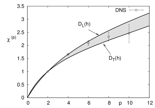
Figure 8: Summary of the Lagrangian Scaling exponents as measured in our DNS in the inertial range of time scales (circles), together with the prediction obtained from the Eulerian statistics by using the bridge relation either with the longitudinal Eulerian statistics (upper limit of the shadowed area) or with the transverse one (lower limit of the shadowed area).

5.2 Dissipative Effects

The possibility to assess Lagrangian data, both numerically and experimentally, opened the way to investigate also dissipative and sub-dissipative time scales. For Eulerian statistics is very difficult to have reliable data at scales smaller then $\eta$, due to either limitations induced by the probe size, for experiments, or by the numerical resolution (see Schumacher (2007); Schumacher et al. (2007); Watanabe & Gotoh (2007); Yamazaki et al. (2002) for recent DNS meant to address this issue). For Lagrangian quantities, the development of non-intrusive experimental techniques (mainly based on fast CCD Toschi & Bodenschatz (2009)) and the advancements of numerical algorithm to track particles, allowed for assessing time fluctuations of the order of $0.1\tau_{\eta}$ even at high Reynolds numbers. Now, new question about the statistical fluctuations for $\tau\sim\tau_{\eta}$ or smaller, arise. Recently, a lot of attention has been payed on the dip region visible in the local Lagrangian scaling exponents as shown in fig. (7) both from numerical and experimental studies (Arneodo et al. (2008)). In the last twenty years, a lot of work has been done to include viscous fluctuations in the multifractal theory – initially for Eulerian statistics– Paladin & Vulpiani (1987); Nelkin (1990); Meneveau (1996); Frisch & Vergassola (1991); Benzi et al. (1991), and more recently also for Lagrangian statistics (Chevillard et al. (2003); Biferale et al. (2004)). A simple way to accomplish this is to take into account of the fact that, according to the MF theory, the viscous scale is not a fixed homogeneous quantity, but fluctuates wildly due to intermittency. Moreover, viscous and inertial fluctuations are linked by the requirement that viscous effects happens when the local Reynolds number becomes ${\cal O}(1)$ as first remarked by Paladin & Vulpiani (1987):

$$\frac{\delta_{\eta}u\;\eta}{\nu}\sim{\cal O}(1);\qquad\eta^{1+h}\sim\nu;\qquad\eta(h)\sim Re^{-1/(1+h)},$$ (20)

where we have taken for simplicity, $L=1,U_{0}=1$ and $\nu=Re^{-1}$. Using the bridge relation (15) we may immediately find out also the equivalent fluctuations relation for the Kolmogorov dissipative time (Biferale et al. (2004)):

$$\tau_{\eta}(h)\sim\eta^{1-h}\sim Re^{(h-1)/(1+h)}.$$ (21)

Taking in to account this fact, one may use a Batchelor-Meneveau like parametrisation (Meneveau (1996); Sirovich et al. (1994); Chevillard et al. (2003); Arneodo et al. (2008)) of velocity increments for all time lags, including the fluctuating viscous time in the game:

$$\delta_{\tau}v=V_{0}\,\frac{\tau}{T_{L}}\left[\left(\frac{\tau}{T_{L}}\right)^{\alpha}+\left(\frac{\tau_{\eta}(h)}{T_{L}}\right)^{\alpha}\right]^{\frac{2h-1}{\alpha(1-h)}}\,,$$ (22)

where $\alpha$ being a free parameter controlling the crossover around $\tau\!\sim\!\tau_{\eta}$, and $V_{0}$ the root mean square large scale velocity. It is easy to realize that the above expression has the correct asymptotic behaviour for very small time lags $\delta_{\tau}v\sim\tau a$, where $a=\delta_{\tau_{\eta}}v\tau_{\eta}$ is the acceleration; and in the inertial range, $\delta_{\tau}v\sim\tau^{h/(1-h)}$, as described in details in Arneodo et al. (2008). In order to get a prediction for the behaviour of the LSF we need also to introduce dissipative effects in the MF probability. This can be done as follows:

$$P_{h}(\tau,\tau_{\eta})={\cal Z}^{-1}(\tau)\left[\left(\frac{\tau}{T_{L}}\right)^{\alpha}+\left(\frac{\tau_{\eta}(h)}{T_{L}}\right)^{\alpha}\right]^{\frac{3-D(h)}{\alpha(1-h)}},$$ (23)

where ${\cal Z}$ is a normalizing function and $D(h)$ the fractal dimension of the support of the exponents $h$ (either $D_{L}(h)$ or $D_{T}(h)$ if one wants to link the Lagrangian dissipative physics to the Eulerian one). At this point, given the Reynolds number, we are left with two parameters ($\alpha$ and a multiplicative constant in the definition of $\tau_{\eta}$). In order to compute the LSF at all time lags one needs to integrate the expression (22) with the weight given by (23) over all possible $h$-values:

$$\langle(\delta_{\tau}v)^{p}\rangle\sim\int_{h_{min}}^{h_{max}}dhP_{h}(\tau)[\delta_{\tau}v(h)]^{p}.$$ (24)

Clearly, the above picture goes back to the inertial values when we have $\tau/T_{L}\rightarrow 0$ and $\tau\gg\tau_{\eta}$, i.e. when we can neglect viscous effects and we can perform the saddle point estimate. Here we do not want to do that, keeping all corrections, and compare the simple parametrisation (22), dressed with the MF theory, with our data. First, let us see what are the qualitative results obtained from (22) at changing the free parameters on it. In fig. (9) we show the results for $\chi^{(p)}(\tau)$ as obtained from the global MF description (24) for $p=4,6,8$ with a fixed $D(h)$ at changing the free parameter $\alpha=4$ (left panel) or $\alpha=2$ (right panel). From this figure we learn two things. The MF description is very close, already qualitatively speaking, to the real data –compare with panel corresponding to $p=4$ of Fig. (7). In particular, the dip present in the data is also captured by the MF. Moreover, at changing the free parameter $\alpha$ one may deplete or enhance the dip intensity, as can be see comparing left and right panel of Fig. (9). Let us also notice that the dip region is entirely due to the presence of the fluctuating viscous cut-off, $\tau_{\eta}(h)$, as can be seen in the inset of right panel of Fig. (9), where the same data but with a fixed $\tau_{\eta}$ are plotted and the dip has disappeared.

Second, from fig. (9) one sees that for any finite Reynolds numbers, there are corrections to scaling induced by the large time lags $T_{L}$; as a consequence, in the inertial range the local exponents are not exactly constant. In order to give a qualitative assessment of the importance of this finite Reynolds corrections as described by formula (22) we plot in the left panel of fig. (10) the values of $\chi^{(4)}(\tau)$ for three different Reynolds numbers. As one can see, at increasing Reynolds, the inertial range values becomes flatter and flatter, as they must do. At difference from what happens in the infinite Reynolds number limits, for any finite Reynolds, the whole support of $D(h)$ will play a role in the integration (24): for not too small $\tau/T_{L}$ the saddle point estimate (18) becomes less and less accurate. As a result, the whole shape of the $D(h)$ curve becomes important for any order.
Indeed, the typical $D(h)$ curve from any MF theory is a convex function like the one used to fit the Eulerian Longitudinal exponents depicted in the inset of right panel of fig. (10). The left part of $D(h)$ curve, with $h\in[h_{min},h_{peack}]$, is connected to the positive order of the Eulerian Structure Functions (Frisch (1995)). The right side, $h\in[h_{peack},h_{max}]$, is connected to negative moments. Negative moments are generally hill defined and one needs to use inverse statistics to assess the right part of the $D(h)$ curve (Jensen (1999); Biferale et al. (1999)). Because of that, we have a good control only the left side, where most of the previous experimental and numerical studies focused. The extension of the integration in (24) over the $h$-value on the right of the peack of $D(h)$ is therefore not based on solid experimental or numerical basis. The extension to the right part of a given functional form for $D(h)$ (log-Poisson, log-Normal etc. ), obtained by fitting only positive moments of Structure functions, is arbitrary.

In the right panel we show the dependence of the final expression (24) from the extension of the integration over the $h$ range. As one can see, the inclusion of $h$-value falling on the right of the peack gives an important contributions to the behaviour of the local slopes for $\tau\sim T_{L}$, confirming the importance of the whole $D(h)$ if one want to control the finite-Reynolds corrections to the saddle point estimate (18). For a more detailed investigation of the property of the MF formulation (24) also compared with other DNS and experimental results, the reader can consult the recent collection of data published in (Arneodo et al. (2008)).

Figure 9: Results for the local Lagrangian exponents, $\chi^{(p)}(\tau)$ as obtained from the finite Reynolds multifractal formula (22-23-24) for a given Reynolds number and $p=4,6,8$, at changing the free parameter, $\alpha$, that sets the importance of the dip region. Left: $\alpha=4$; Right: $\alpha=2$. In the inset of the right panel we also show, $\chi^{(4)}(\tau)$ obtained from the same multifractal formula but keeping fixed the dissipative time scales, $\tau_{\eta}(h)=const.$, in this latter case the dip region disappears.

Figure 10: Left panel: Reynolds effects on the local exponents predicted from the MF interpolation formula (22-23-24), we kept fixed everything except the Reynolds numbers. Right: sensitivity to the whole shape of the $D(h)$ curve of the $\chi^{(4)}(\tau)$ as predicted from the MF interpolation formula. We show two cases. One case is obtained integrating only on fluctuations in the left region of the $D(h)$ curve with respect to its peack, $h\in[h_{min},h_{max}]$, with $h_{max}=h_{peack}=0.38$, the second case consider also smoother fluctuations up to $h_{max}=0.5$.The typical log-Poisson shape of the $D(h)$ used is depicted in the inset.

6 Conclusions

We have reported about Eulerian and Lagrangian statistics from high resolution Direct Numerical Simulations of isotropic weakly compressible turbulence. Reynolds number at the Taylor microscale is estimated to be around $600$. The high number of particle trajectories explored, together with the high resolution Eulerian flow allowed us for the first time to study Lagrangian intermittency up to moments of order $p=10$, at large Reynolds numbers. The four main results we have presented are: (i) Eulerian Longitudinal and Transverse statistics have slightly different scaling properties, in agreement with previous incompressible DNS data at comparable resolution. (ii) Lagrangian statistics is more intermittent than Eulerian ones, percentage-wise with respect to the observed deviations from dimensional scaling and its quantitative value can be captured by using a simple multifractal bridge relations. (iii) In order to correctly asses Lagrangian scaling properties is mandatory to make a scale-by-scale analysis, in order to disentangle the dip region close to viscous scales from the inerital range interval. A lack of such analysis may lead to an underestimate of the Lagrangian scaling exponents, because of the strong intermittency of the dip interval, dominated by viscous effects.(iv) Multifractal phenomenology, is able to describe in a unified way: dissipative effects, inertial range fluctuations and large scale corrections (Arneodo et al. (2008)).
This study leaves open a few important questions. First, we need to wait for higher Reynolds numbers data, in highly isotropic ensemble, to resolve the riddle about Longitudinal versus Transverse Eulerian fluctuations. Second, we need to collect also data with higher Lagrangian statistics to understand whether the Eulerian-Lagrangian bridge relation remains valid for higher moments. Third, it is important to improve experimental and numerical accuracy to measure small-scales and small-time fluctuations, where highly non trivial physics is developing as shown by the strong enhancement of local intermittency in the dip region $\tau\in[1:10]\tau_{\eta}$. Such strong enhancement of fluctuations around the viscous scale is due to local fluctuations of the dissipative cut-off, which reflects in to the existence of different viscous effects for different moments and different correlation functions (Frisch & Vergassola (1991); L’vov & Procaccia (1996); Yakhot & Sreenivasan (2004); Benzi & Biferale (2009)). It is well described, within the multifractal theory, by the Paladin-Vulpiani relation (20), as shown by the fact that the dip region disappear by removing the viscous fluctuations in (22-23), see inset of the right side of fig. (9). Such effect is probably the highest difficulty to overcome in both stochastic modeling (Sawford (2001)) and theory of Lagrangian turbulence (Yakhot (2009); Zybin et al. (2008)).

We acknowledge very useful discussions with M. Cencini, A. Lanotte, L. Kadanoff and V. Yakhot. L.B., R.B. and F.T. thank the Flash Center at the University of Chicago for hospitality when part of this work was prepared. We also want to thank B. Gallagher for helping in the data analysis and data rendering.

References

- Arneodo et al. (1996) Arneodo, A. et al. 1996. Structure functions in turbulence, in various flow configurations, at Reynolds number between 30 and 5000, using extended self-similarity. Europhys. Lett. 34, 411.
- Arneodo et al. (2008) Arneodo, A. et al. 2008. Universal Intermittent Properties of Particle Trajectories in Highly Turbulent Flows. Phys. Rev. Lett 100, 254504.
- Bec et al. (2006) Bec, J., Biferale, L., Cencini, M., Lanotte, A. & Toschi, F. 2006. Effects of vortex filaments on the velocity of tracers and heavy particle in turbulence. Phys. Fluids 18, 081702.
- Belinicher et al. (1998) Belinicher V.I., L’vov, V., Pomyalov, A. & Procaccia, I. 1998. Computing the Scaling Exponents in Fluid Turbulence from First Principles: Demonstration of Multiscaling. J. Stat. Phys., 93 797 - 832.
- Benzi et al. (1991) Benzi, R., Biferale, L., Paladin, G., Vulpiani, A. & Vergassola, M. 1991. Multifractality in the statistics of the velocity gradients in turbulence. Phys. Rev. Lett. 67, 2299.
- Benzi et al. (1993) Benzi, R. et al. 1993. Extended self-similarity in turbulent flows. Phys. Rev. E 48, R29.
- Benzi et al. (1996) Benzi, R. et al. 1996. Generalized scaling in fully developed turbulence. Physica D 96, 162.
- Benzi et al. (1998) Benzi, R., Biferale, L. & Toschi, F.. 1998. Multiscale velocity correlations in turbulence. Phys. Rev. Lett. 80, 3244.
- Benzi et al. (2008) Benzi,R., Biferale, L., Fisher, R., Kadanoff, L., Lamb, D. & Toschi, F. 2008. Intermittency and Universality in Fully-Developed Inviscid and Weakly-Compressible Turbulent Flows. Phys Rev Lett 100, 234503.
- Benzi & Biferale (2009) Benzi, R. & Biferale, L. 2009. Fully developed turbulence and the multifractal conjecture. Journ. Stat. Phys. (to appear).
- Berg et al. (2006) Berg, J., Luthi, B., Mann, J. & Ott, S. 2006. Backwards and forwards relative dispersion in turbulent flow: an experimental investigation. Phys. Rev. E 74 016304.
- Biferale et al. (1999) Biferale, L., Cencini, M., Vergni, D. & Vulpiani, A.1999 Exit time of turbulent signals: A way to detect the intermediate dissipative range. Rev. E 60, R6295.
- Biferale et al. (2004) Biferale, L. et al. 2004. Multifractal statistics of Lagrangian velocity and acceleration in turbulence. Phys. Rev. Lett. 93, 064502.
- Biferale et al. (2005) Biferale, L., Boffetta, G., Celani, A., Lanotte, A. & Toschi, F. 2005. Particle trapping in three-dimensional fully developed turbulence. Phys. Fluids 17, 021701.
- Biferale et al. (2008) Biferale, L., Bodenschatz, E., Cencini, M., Lanotte, A., Ouellette, N., Toschi, F. & Xu, H. 2008. Lagrangian structure functions in turbulence: A quantitative comparison between experiment and direct numerical simulation. Phys . Fluids 20, 065103.
- Biferale & Procaccia (2005) Biferale, L. & Procaccia, I.2005. Anisotropy in Turbulent Flows and in Turbulent Transport. Phys. Rep. 414, 43.
- Biferale (2008) Biferale, L. 2008. A note on the fluctuation of dissipative scale in turbulence. Phys. Fluids 20 , 031703.
- Boffetta et al. (2002) Boffetta, G., De Lillo, F. & Musacchio, M. 2002. Lagrangian statistics and temporal intermittency in a shell model of turbulence. Phys. Rev. E 66, 066307.
- Boffetta et al. (2008) Boffetta, G., Mazzino, A. & Vulpiani,A. 2008. Twenty-five years of multifractals in fully developed turbulence: a tribute to Giovanni Paladin. J. Phys. A: Math. Theor. 41 363001.
- Boratav & Pelz (1997) Boratav, O.& Pelz, R. 1997. Structures and structure functions in the inertial range of turbulence. Phys Fluids 9, 1400.
- Borgas (2003) Borgas, MS. 1993. The Multifractal Lagrangian Nature of Turbulence. Phil. Trans. R. Soc. London A 342, 379.
- Bourgoin et al. (2006) Bourgoin, M., Ouelette, N., Xu, H., Berg, J. & Bodenschatz, E. 2006. The role of pair dispersion in turbulent flow. Science 311 835.
- Chen et al. (1997) Chen, S., Sreenivasan, K.R. & Nelkin, M. 1997. Inertial range scalings of dissipation and enstrophy in isotropic turbulence. Phys. Rev. Lett. 79, 2253.
- Chevillard et al. (2003) Chevillard, L., Roux, S,. Leveque, E., Mordant, N., Pinton, J.-F. & Arneodo, A. 2003. Lagrangian velocity statistics in turbulent flows: Effects of dissipation. Phys. Rev. Lett. 91, 214502.
- Dhruva et al. (1997) Dhruva, B., Tsuji, Y. & Sreenivasan, K.R. 1997. Transverse structure functions in high-Reynolds-number turbu- lence. Phys. Rev. E 56 R4928.
- Dubrulle (1994) Dubrulle, B. 1994. Intermittency in fully developed turbulence: Log-Poisson statistics and generalized scale covariance. Phys. Rev. Lett. 73, 959.
- Fisher et al. (2007) Fisher, R. et al. 2007. Terascale Turbulence Computation on BG/L Using the FLASH3 Code. IBM Journ. Res. Devel. 52 127.
- Frisch (1995) Frisch, U. 1995. Turbulence: the legacy of A.N. Kolmogorov (Cambridge University Press, Cambridge UK).
- Frisch & Vergassola (1991) Frisch, U.& Vergassola, M. 1991. A prediction of the multifractal model – The intermediate dissipation range. Europhys. Lett. 14, 439.
- Gotoh et al. (2002) Gotoh, T., Fukayama,D. & Nakano, T.2002. Velocity field statistics in homogeneous steady turbulence obtained using a high-resolution direct numerical simulations. Phys. Fluids 14, 1065.
- Jensen (1999) Jensen, M.H. 1999. Chaotic Dynamics Title: Multiscaling and Structure Functions in Turbulence: An Alternative Approach. Phys. Rev. Lett. 83, 76.
- He et al. (1998) He, G., Chen, S., Kraichnan, R.H., Zhang, R. & Zhou, Y. 1998. Statistics of dissipation and enstrophy induced by localized vortices. Phys Rev. Lett 81, 4636.
- Hill (2001) Hill, R. 2001. Equations relating structure functions of all orders. J. Fluid Mech. 434, 379.
- Homann et al. (2007) Homann, H., Grauer, R.,Busse, A. & Mueller, W. 2007 Lagrangian statistics of Navier-Stokes and MHD turbulence. J. Plasma Physics 73, 821.
- Ishihara et al. (2009) Ishihara, T., Gotoh, T. & Kaneda, Y. 2009 Study of High-Reynolds Number Isotropic Turbulence by Direct Numerical Simulation. Ann. Rev .Fluid Mech. 41 165.
- La Porta et al. (2001) La Porta, A., Voth, G.A., Crawford, A.M., Alexander, J. & Bodenschatz, E. 2001. Fluid particle accelerations in fully developed turbulence. Nature 409 1017.
- Lohse (1994) Lohse, D. 1994. Crossover from high to low-Reynlds-number turbulence Phys. Rev. Lett. 73 3223.
- Luthi et al. (2005) Luthi B, Tsinober A, Kinzelbach W. 2005. Lagrangian measurement of vorticity dynamics in turbulent flow. J. Fluid Mech. 528 87.
- Berg et al. (2009) Berg, J., Ott, S., Mann, J. & Luthi, B. 2009. Lagrangian structure functions in a turbulent flow at intermediate Reynolds number. arXiv:0903.2633 physics.flu-dyn.
- L’vov & Procaccia (1996) L’vov, V.S. & Procaccia, I. 1996. Viscous lengths in hydrodynamic turbulence are anomalous scaling functions. Phys. Rev. Lett. 77 3541.
- Jimenez et al. (1993) Jimenez, J., Wray, A.A., Saffman, P.G. & Rogallo, R.S. 1993. The structure of intense vorticity in isotropic turbulence. J. Fluid Mech.255 65.
- Mazzitelli & Lohse (2004) Mazzitelli, I. & Lohse, D. 2004. Lagrangian statistics for fluid particles and bubbles in turbulence. New J. Phys. 6, 203.
- Meneveau (1996) Meneveau, C. 1996. Transition between viscous and inertial-range scaling of turbulence structure functions. Phys. Rev. E 54, 3657.
- Mordant et al. (2001) Mordant, N., Metz, P., Michel, O. & Pinton, J.-F., 2001. Measurement of Lagrangian Velocity in Fully Developed Turbulence. Phys. Rev. Lett. 87, 214501.
- Mordant et al. (2006) Mordant, N., Leveque, E. & Pinton, J.-F. 2006. Experimental and Numerical Study of Lagrangian dynamics of high Reynolds Turbulence. New J.Phys. 6 116.
- Nelkin (1990) Nelkin,M. 1990. Multifractal scaling of velocity derivatives in turbulence. Phys. Rev. A 42, 7226.
- Ott & Mann (2000) Ott, S. & Mann, J. 2000. An experimental investigation of the relative diffusion of particle pairs in three- dimensional turbulent flow. J. Fluid Mech. 422 207.
- Paladin & Vulpiani (1987) Paladin,G. & Vulpiani, A. 1987. Degrees of freedom of turbulence. Phys. Rev. A 35, R1971.
- Parisi & Frisch (1985) Parisi, G. & Frisch, U. in Turbulence and Predictability in Geophysical Fluid Dynamics, Proceed. Intern. School. of Physics “E. Fermi”. eds. Ghil M, Benzi R, Parisi G. 84–87. (1985).
- Porter et al. (2002) Porter, D., Pouquet, A. &. Woodward, P. 2002. Measures of intermittency in driven supersonic flows. Phys. Rev. E 66, 026301.
- Sawford (2001) Sawford, B.L. 2001. Turbulent relative dispersion. Annu. Rev. Fluid Mech. 33 289.
- Schumacher (2007) Schumacher, J. 2007. Sub-Kolmogorov-scale fluctuations in Fluid Turbulence. Europhys. Lett. 80, 54001.
- Schumacher et al. (2007) Schumacher, J., Sreenivasan, K.R. & Yakhot, V. 2007. Asymptotic exponents from low-Reynolds-number flows. New J. Phys. 9, 89.
- She & Leveque (1994) She, Z.-S. & Leveque, E. 1994. Universal scaling laws in fully developed turbulence. Phys. Rev. Lett. 72, 336.
- Shen & Warhaft (2002) Shen X, Warhaft Z. 2002. Longitudinal and transverse structure functions in sheared and unsheared wind-tunnel turbulence. Phys. Fluids 14 370.
- Sirovich et al. (1994) Sirovich, L., Smith, L. & Yakhot, V. 1994. Energy spectrum of homogeneous and isotropic turbulence in far dissipation range. Phys. Rev. Lett. 72, 344.
- Toschi & Bodenschatz (2009) Toschi, F. & Bodenschatz, E. 2009. Lagrangian properties of particles in turbulence. Annu. Rev. Fluid Mech. 41 375.
- van der Water (1999) van de Water, W. & Herweijer J.A. 1999. High-order structure functions of turbulence. J. Fluid Mech. 387 3.
- Xu et al. (2006) Xu, H., Bourgoin, M., Ouellette, N.T. & Bodenschatz, E. 2006. High order Lagrangian velocity statistics in turbulence. Phys. Rev. Lett. 96, 024503.
- Yakhot & Sreenivasan (2004) Yakhot, V. & Sreenivasan, K.R. 2004. Towards a dynamical theory of multifractals in turbulence. Physica A 343, 147.
- Yakhot & Sreenivasan (2005) Yakhot, V. & Sreenivasan, K.R. 2005. Anomalous scaling of structure functions and dynamic constraints on tur- bulence simulations. J. Stat. Phys. 121 823.
- Yakhot (2009) Yakhot, V private communication (unpublished).
- Yamazaki et al. (2002) Yamazaki, Y., Ishihara, T. & Kaneda, Y. 2002. Effects of wavenumber truncation on high-resolution direct numerical simulation of turbulence. J. Phys. Soc. Jpn. 71 777.
- Yeung et al. (2006) Yeung, P.K., Pope, S.B. & Sawford, B.L. 2006. Reynolds number dependence of Lagrangian statistics in large numerical simulations of isotropic turbulence. J. Turbul. 7 N58.
- Watanabe & Gotoh (2007) Watanabe, T. & Gotoh, T. 2007. Inertial-range intermittency and accuracy of direct numerical simulation for turbulence and passive scalar turbulence. J. Fluid Mech. 590 117.
- Zhou & Antonia (2000) Zhou, T. & Antonia, R.A. 2000. Reynolds number dependence of the small-scale structure of grid turbulence. J. Fluid Mech. 406 81.
- Zybin et al. (2008) Zybin, K., Sirota, V.A., Ilyin, A.S. & Gurevich, A.V. 2008. Lagrangian statistical theory of fully developed hydrodynamical turbulence. Phys. Rev. Lett. 100, 174504.