Elastic effects of liquids on surface physics

Abstract

The contact between a liquid and an elastic solid generates a stress vector depending on the curvature tensor in each point of the separating surface. For nanometer values of the mean curvature and for suitable materials, the stress vector takes significant amplitude on the surface. Although the surface average action of the liquid on the solid is the hydrostatic pressure, the local strain generates torques tending to regularize the surface undulations and asperities.

1 Introduction

In 1977, John Cahn gave simple illuminating arguments to describe the interaction between solids and liquids. His model was based on a generalized van der Waals theory of fluids treated as attracting hard spheres [1]. It entailed assigning an energy to the solid surface that is a functional of the liquid density at the surface. It was thoroughly examined in a review paper by de Gennes [2]. Three hypotheses are implicit in Cahn’s picture:  i)  The liquid density is taken to be a smooth function of the distance from the solid surface, that surface is assumed to be flat on the scale of molecular sizes and the correlation length is assumed to be greater than intermolecular distances;  ii)  The forces between solid and liquid are of short range with respect to intermolecular distances;  iii)  The liquid is considered in the framework of a mean-field theory. This means, in particular, that the free energy of the liquid is a classical so-called gradient square functional.
The point of view that the liquid in an interfacial region may be treated as bulk phase with a local free-energy density and an additional contribution arising from the nonuniformity which may be approximated by a gradient expansion truncated at the second order, is most likely to be successful and perhaps even quantitatively accurate near the liquid critical point [3]. We use this approximation enabling us to compute analytically the liquid density profiles. Nevertheless, we take surface effects and repulsive forces into account by adding density functionals at boundary surfaces. In mean-field theory, London potentials of liquid-liquid and liquid-solid molecular interactions are

$$\left\{\begin{array}[]{c}\displaystyle\;\;\;\;\;\;\varphi_{ll}=-\frac{c_{ll}}{r^{6}}\;,\text{ \ when\ }r>\sigma_{l}\;\;\text{and }\;\ \varphi_{ll}=\infty\text{ \ when \ }r\leq\sigma_{l}\,,\\ \displaystyle\;\;\;\;\;\;\varphi_{ls}=-\frac{c_{ls}}{r^{6}}\;,\text{ \ when\ }r>\delta\;\;\text{and }\;\ \varphi_{ls}=\infty\text{ \ when \ }r\leq\delta\;,\end{array}\right.$$

where $c_{ll}$ et $c_{ls}$ are two positive constants associated with Hamaker constants, $\sigma_{l}$ and $\sigma_{s}$ respectively denote liquid and solid molecular diameters, $\delta=\frac{1}{2}($ $\sigma_{l}+$ $\sigma_{s})$ is the minimal distance between centers of liquid and solid molecules [4].

We consider the interaction between a solid surface flat at a molecular scale (but curved at several nanometer scale) and a liquid by means of a continuous model. The density-functional of energy $E$ of the inhomogeneous liquid in a domain $D$ of differentiable boundary $S$ (external forces being neglected) is taken in the form

$$E=E_{f}+E_{S}\qquad{\mathrm{with}\qquad\emph{E}_{\emph{f}}=\int\int\int_{D}\rho\,\varepsilon\ dv,\ \emph{E}_{\emph{S}}\ =\ \int\int_{S}\phi\ ds}.$$

The first integral (energy of the volume) is associated with square-gradient approximation when we introduce a specific free energy of the fluid at a given temperature, $\varepsilon=\varepsilon(\rho,\beta)$, as a function of liquid density $\rho$ and $\beta=(\mathrm{grad\,\rho)^{2}}$. Specific free energy $\varepsilon$ characterizes together fluid properties of compressibility and molecular capillarity of interfaces. In accordance with gas kinetic theory [5], scalar $\lambda=2\rho\,\varepsilon_{,\beta}(\rho,\beta)$ (where $\varepsilon_{,\beta}$ denotes the partial derivative with respect to $\beta$) is assumed to be constant at a given temperature and

$$\rho\,\varepsilon=\rho\,\alpha(\rho)+\frac{\lambda}{2}\,(\text{grad\ }\rho)^{2},$$

where term $({\lambda}/{2})\,(\mathrm{grad\ \rho)^{2}}$ is added to the volume free energy $\rho\,\alpha(\rho)$ of a compressible fluid. We denote the pressure term by $P(\rho)=\rho^{2}\alpha^{\,\prime}(\rho).$ The second integral (energy of the surface) is such that the free energy per unit surface $\phi$ is [2],

$$\phi(\rho)=-\gamma_{1}\rho+\frac{1}{2}\,\gamma_{2}\,\rho^{2}.$$ (1)

Here $\rho$ denotes the limit liquid density value at surface $S$. Constants $\gamma_{1}$, $\gamma_{2}$ and $\lambda$ are positive and given by relations [6],

$$\gamma_{1}=\frac{\pi c_{ls}}{12\delta^{2}m_{l}m_{s}}\;\rho_{sol},\quad\gamma_{2}=\frac{\pi c_{ll}}{12\delta^{2}m_{l}^{2}},\quad\lambda=\frac{2\pi c_{ll}}{3\sigma_{l}\,m_{l}^{2}},$$

where $m_{l}$ et $m_{s}$ respectively denote the masses of liquid and solid molecules; $\rho_{sol}$ is the solid density.

In this paper, we first develop the boundary conditions for the general case of the interaction between a non-homogeneous liquid and a curved solid surface with a surface energy due to intermolecular interactions and depending of the fluid volume deformation. Then, for a surface energy in form (1) we study the stress vector distribution on a surface where bumps and hollows are periodically distributed. Finally, we estimate the stress effects for a silicon surface, with a curvature of several nanometer range, in contact with water.

2 Boundary conditions

The equation of equilibrium and boundary conditions are obtained by using the virtual power principle [7, 8]. For example, virtual displacements ${\mathbf{\zeta}}=\delta\mathbf{x}$ are defined in a classical way by Serrin [9] page 145, where $\mathbf{x}=\{x^{i}\},(i=1,2,3)$ denotes the Euler variables in a Galilean or fixed system of coordinates.

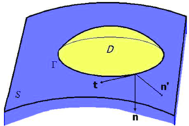
Figure 1: Vector $\mathbf{n}$ is the unit normal vector to $S$ exterior to $D$; vector $\mathbf{t}$ is the unit tangent vector to $\Gamma$ with respect to $\mathbf{n}$; ${\mathbf{n}^{\prime}}={\mathbf{t}}\times{\mathbf{n}}$.

A liquid (in drop form) occupying a domain $D$ of the physical space lies on a solid surface $S$ (the liquid is also partially bordered by a gas); the edge $\Gamma$ (or contact line) is the curve common to $S$ and the boundary of $D$ (see Fig. 1). All the surfaces and curves are oriented differential manifolds ().

2.1 Variation of the density-functional of energy $E$

The density in the fluid has a limit value at the wall $S$. Then, on $S$,

$$\delta\phi=\phi^{\prime}(\rho)\,\delta\rho=-\rho\,\phi^{\prime}(\rho)\,\mathrm{div}\,{\mathbf{\zeta}},$$

where $\delta\rho+\rho\,\mathrm{div}\,{\mathbf{\zeta}}=0$ [9]. Let us denote

$$G=-\rho\,\phi^{\prime}(\rho)\,,\quad H=\phi(\rho)-\rho\,\phi^{\prime}(\rho).$$

The function $H$ is the Legendre transform of $\phi$ with respect to $\rho$. For any virtual displacement ${\mathbf{\zeta}}$ null on $\Gamma$, Rel. (11) of Appendix yields,

$$\int\int_{S}\delta\phi\ ds=\int\int_{S}G\ \mathrm{div}\,{\mathbf{\zeta}}\ ds\equiv\displaystyle\int\int_{S}\ \left\{G\,\frac{d\zeta_{n}}{dn}-\left(\frac{2G}{R_{m}}\,{\mathbf{n}}^{T}+\mathrm{grad}_{tg}^{T}G\right){\mathbf{\zeta}}\right\}ds,$$

where, now $S$ is the imprint of $D$ on the solid surface. Consequently, from the calculations in Appendix, we obtain:
For any virtual displacement null on the complementary boundary of $D$ with respect to $S$ and null on the edge $\Gamma$, the variation of $E$ is,

$$\begin{array}[]{ll}\delta E=\displaystyle-\int\int\int_{D}(\mathrm{div}\,\sigma)\,{\mathbf{\zeta}}\,dv&\\ +\displaystyle\int\int_{S}(G-A)\frac{d{\zeta}_{n}}{dn}+\left(\frac{2(A-H)}{R_{m}}\,{\mathbf{n}}^{T}+\mathrm{grad}_{tg}^{T}(A-H)+{\mathbf{n}}^{T}\sigma\right){\mathbf{\zeta}}\ ds,&\end{array}$$

where

$$\ \sigma=-p\,{I}-\lambda\ \mathrm{grad}\;\rho\otimes\mathrm{grad}\;\rho\equiv-p\,{I}-\lambda\,\left(\frac{\partial\rho}{\partial{\mathbf{x}}}\right)^{T}\frac{\partial\rho}{\partial{\mathbf{x}}}$$ (2)

is the symmetric stress tensor of the inhomogeneous liquid, with $p=\rho^{2}\varepsilon_{,\rho}-\rho\ \mathrm{div}(\lambda\mathrm{\ grad}\,\rho)$ ; $A=\lambda\,\rho\,\left({d\rho}/{dn}\right)$ with$\ {d\rho}/{dn}=\left({\partial\rho}/{\partial{\mathbf{x}}}\right)\,{\mathbf{n}}$ ; ${\zeta}_{n}={\mathbf{n}}^{T}\,{\mathbf{\zeta}}$ ; $2/R_{m}$ is the mean curvature of $S$ and $\mathrm{grad}_{tg}$ denotes the tangential part of the gradient relatively to $S$.

2.2 The virtual work of forces exerted on $D$

The virtual work of elastic stresses on $S$ is

$$\delta\tau_{e}=\int\int_{S}{\mathbf{\kappa}}^{T}{\mathbf{\zeta}}\ ds\,,$$

where ${\mathbf{\kappa}}={-\sigma_{e}}\,{\mathbf{n}}$ is the loading vector associated with stress tensor $\sigma_{e}$ on the wall in classical theory of continuum mechanics (). Then, the virtual work of forces $\delta\tau$ exerted on $D$ is $\delta\tau=-\,\delta E+\delta\tau_{e}\,$ and,

$$\begin{array}[]{ll}\delta\tau=\displaystyle\int\int\int_{D}(\mathrm{div}\,\sigma)\,{\mathbf{\zeta}}\,dv&\\ -\displaystyle\int\int_{S}(G-A)\frac{d{\zeta}_{n}}{dn}+\left(\frac{2(A-H)}{R_{m}}\,{\mathbf{n}}^{T}+\mathrm{grad}_{tg}^{T}(A-H)+{\mathbf{n}}^{T}\sigma-{\mathbf{\kappa}}^{T}\right){\mathbf{\zeta}}\ ds.&\end{array}$$

2.3 Results

The fundamental lemma of variation calculus, applied to the relation $\delta\tau=0$, for all previous virtual displacements, yields:

$\bullet$  The well-known equation of equilibrium for capillary fluids [10],

$$\mathrm{div}\,\sigma=0,$$ (3)

$\bullet$  The boundary conditions on $S$,

$$\forall\ {\mathbf{x}}\in S,\ \ \ \ \ \ \ \ \ \left\{\begin{array}[]{l}G-A=0,\\ {\mathbf{\kappa}}=\,\displaystyle\frac{2(A-H)}{R_{m}}\;{\mathbf{n}}+\mathrm{grad}_{tg}(A-H)+\sigma\;{\mathbf{n}}.\end{array}\right.$$ (4)

Equation (4)₁ yields a condition relative to the surface energy (1) which depends on the fluid density at the surface and on the quality of the solid wall:

$$\lambda\ \frac{d\rho}{dn}+\phi^{\prime}(\rho)=0\qquad\mathrm{or}\qquad\lambda\,\frac{d\rho}{dn}=\gamma_{1}-\gamma_{2}\,\rho\,.$$ (5)

Equation (5) expresses an embedding effect for the liquid density. Such a condition appears for simpler geometry in [1, 11].
Condition (4)₂ appears in the literature [7, 12] but without the terms corresponding to the molecular model (1) of surface free energy. Such type of condition also appears in interfacial problems with other solid surface energy but with a null curvature as in [1, 11]. In Cauchy theory, we are back to the classical equation ${\mathbf{\kappa}}=\sigma\;{\mathbf{n}}$.
The definition (2) of $\sigma$ implies $\sigma\,{\mathbf{n}}=-p\,{\mathbf{n}}-\lambda\;({d\rho}/{dn})\ \mathrm{grad}\;\rho\,.$ Then, for an elastic wall, by taking into account of Rel. (5), the vector $\mathbf{\kappa}$ is normal to $S$,

$${\mathbf{\kappa}}=\kappa_{n}\,{\mathbf{n}}\quad\mathrm{with}\quad\kappa_{n}\ =\mathbf{n}^{T}\sigma\,\mathbf{n}-\frac{2\,\phi}{R_{m}}\,.$$ (6)

We obtain the stress vector values of the solid at the elastic wall (which is opposite to the action ${\mathbf{\tau}}$ of the liquid on the elastic wall). Relation (6) looks like the Laplace formula for fluid interfaces. Nonetheless, we will see in the next section some differences between the results for fluid interfaces and for liquid-solid interfaces.

3 An example of elastic effect on a solid surface

3.1 General considerations

As bibliography about elastic effects on surface physics, one may refer to the review article [13].
The aim of this section is to present an example of system such that the mesoscopic effects of a liquid locally generate important molecular stress vectors on a solid surface. We consider a periodic domain such that the substrate solid surface has an alternated structure. The solid surface can be considered as a flat domain at the Angström scale because roughness and undulations are only of several nanometer length (such a model is presented on Fig. 2).

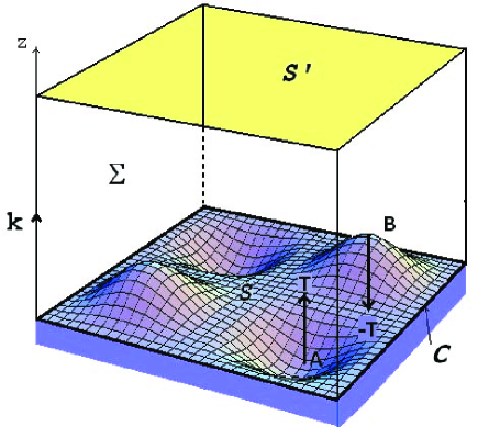
Figure 2: We consider the model consisting of a surface $S$ with bumps and hollows periodically distributed on a period $L$ of several nanometers in two directions such that, with respect to the third axis, the bump and hollow levels are opposite. Extrema of the surface mean curvature are located at point A and B; curve $C$ is the limit curve of the periodic rectangular parallepiped. Surface $S^{\prime}$ delimits the liquid bulk (at a distance $h$ of a great number of nanometers from surface $S$). Surface $\Sigma$ is the lateral boundary of $D$. Vector $\mathbf{k}$ is normal to $S^{\prime}$ and $z$ is directed along $\mathbf{k}$.

At level 0 with respect to the third axis, the lateral boundary of domain $D$ follows the curve $C$ of the bludging surface. Due to the axial symmetries around the lines A$\mathbf{k}$ and B$\mathbf{k}$, in local coordinates with these lines as third axis, $\mathrm{{grad}\,\rho=(d\rho/dz)\mathbf{k}}$ and on these lines the stress tensor $\sigma$ of the inhomogeneous liquid gets expressions in the form

$$\mathbf{\sigma}=\left[\begin{array}[]{ccc}a_{1}&0&0\\ 0&a_{2}&0\\ 0&0&a_{3}\end{array}\right],\quad\mathrm{with}\quad\left\{\begin{array}[]{lll}a_{1}&=&a_{2}=-p,\quad\displaystyle p=P(\rho)-\frac{\lambda}{2}\left(\frac{d\rho}{dz}\right)^{2}-\lambda\,\rho\,\Delta\rho\\ a_{3}&=&\displaystyle{-p-\lambda\left(\frac{d\rho}{dz}\right)^{2},}\end{array}\right.$$

where $\Delta$ is the Laplace operator. Consequently, on these lines, Eq. (3) yields a constant value for the eigenvalue $a_{3}$,

$$p+\lambda\left(\frac{d\rho}{dz}\right)^{2}=P_{l},$$ (7)

where $P_{l}$ denotes the uniform pressure in the liquid bulk of density $\rho_{l}$ bounding the liquid layer at level $h$.
-  Due to symmetries of domain $D$, we deduce the average stress actions of the liquid on $S$ and $S^{\prime}$ are opposite and numerically equal to the pressure $P_{l}$.
-  From Rels. (5-7) we obtain, at points A and B, a stress vector ${\mathbf{\tau}}=-{\mathbf{\kappa}}$, action of the liquid on the elastic wall in the same form than the Laplace formula form for fluid interfaces,

$${\mathbf{\tau}}=\left(P_{\ell}+\frac{2\,\phi}{R_{m}}\right)\,\mathbf{n}.$$ (8)

-  We must emphasize that Rel. (8) is only valid at points A and B. In fact, Rel. (6) yields

$${\mathbf{\tau}}=\left(-\mathbf{n}^{T}\sigma\,\mathbf{n}+\frac{2\,\phi}{R_{m}}\right)\,\mathbf{n},$$ (9)

but for points which are not the summits of bumps or the bottoms of hollows, $-\mathbf{n}^{T}\sigma\,\mathbf{n}\equiv p+\lambda\left({d\rho}/{dn}\right)^{2}\neq P_{\ell}$ where $\lambda({d\rho}/{dn})^{2}\neq\lambda\left(\mathrm{grad}\rho\right)^{2}$. Consequently at a mesoscopic scale, due to the anisotropy of the liquid on curved solid surfaces, Rel. (9) replaces Laplace’s formula of fluid interfaces.
-  The stress vector is directed as $\mathbf{k}$ at points A and B. Due to the axial symmetries around the surface extrema at points A and B and opposite mean curvatures, when we neglect $P_{l}$ with respect to $2\phi/R_{m}$, the stress vector associated with the hollow corresponding to point A is a vector $\mathbf{T}$ parallel to $\mathbf{k}$ and the stress vector associated with the bump corresponding to point B is a vector $\mathbf{-T}$; the two vectors generate a torque on the surface. This result is in accordance with results in [14] where the interaction between liquid and solid is represented as localized dipoles and monopoles depending on bumps and hollows of the surface $S$.

3.2 Application to explicit materials

At $\theta=20{{}^{\circ}}$ Celsius, we consider water damping a wall in silicon. The experimental estimates of coefficients defined in Section 1 are presented in Table 1.
Far from the liquid critical point, the liquid density at the wall is closely the same than the liquid density in the bulk [16].

If we consider a mean radius of curvature of surface S, $R_{m}=-10^{-6}$ cm at point A and $R_{m}=10^{-6}$ cm at point B, when we neglect $P_{l}$, we immediately obtain an arithmetic value of $\tau_{n}\equiv{\mathbf{n}}^{T}{\mathbf{\tau}}=10^{8}$ cgs (or 100 atmospheres) corresponding to stress effects of large magnitude between areas around points A and B.

Physical constants $c_{ll}$ $\sigma_{l}$ $m_{l}$ $\rho_{l}$ Water $1.4\times 10^{-58}$ $2.8\times 10^{-8}$ $2.99\times 10^{-23}$ $0.998$ Physical constants $c_{ls}$ $\sigma_{s}$ $m_{s}$ $\rho_{sol}$ Silicon $1.4\times 10^{-58}$ $2.7\times 10^{-8}$ $4.65\times 10^{-23}$ $2.33$ Deduced constants $\delta$ $\lambda$ $\gamma_{1}$ $\gamma_{2}$ Results (water-silicon) $2.75\times 10^{-8}$ $1.17\times 10^{-5}$ $81.2$ $54.2$

Table 1: The physical values associated with water and silicon are obtained in references [4, 15] and expressed in c.g.s. units (centimeter, gramme, second). No information is available for water-silicon interactions; we assume that $c_{ll}=c_{ls}$.

The elastic effects of a liquid on a solid surface result from the topology of the contact interface. It is amazing to observe that a solid surface considered as an interface between solid and liquid does not require new concept but only a supplementary surface energy and likewise surface morphology.
An important assumption in the previous calculations is that three scales infer in the surface physics: a length scale of one nanometer associated with molecular effects and the expression of surface energy, a length scale of ten nanometers associated with the size of undulations and surface roughness and a length scale of one hundred nanometers associated with the distance of the liquid bulk to the surface $S$.

4 Appendix

Let $S$ be a differentiable oriented manifold in the 3-dimensional space and ${\mathbf{n}}$ its oriented unit normal locally extended in the vicinity of $S$ by the expression ${\mathbf{n(x)}}=\mathrm{grad}\ d(\mathbf{x}),$ where $d(\mathbf{x})$ is the distance of point $\mathbf{x}$ to $S$; covectors $\mathrm{grad}^{T}a$ and $\mathrm{grad}_{tg}^{T}a$ denote the transposition of $\mathrm{grad}\,a$ and $\mathrm{grad}_{tg}a$, respectively; for any vector field ${\mathbf{w}}$, we get [7]:
$\displaystyle\mathrm{rot}({\mathbf{n}}\times{\mathbf{w}})={\mathbf{n}}\,\mathrm{div}\,{\mathbf{w}}-{\mathbf{w}}\,\mathrm{div}\,{\mathbf{n}}+\frac{\partial{\mathbf{n}}}{\partial{\mathbf{x}}}\,{\mathbf{w}}-\frac{\partial{\mathbf{w}}}{\partial{\mathbf{x}}}\,{\mathbf{n}}.$
From $\,\displaystyle{\mathbf{n}}^{T}\frac{\partial{\mathbf{n}}}{\partial{\mathbf{x}}}=0\,$ and $\,\mathrm{div}\,{\mathbf{n}}=\displaystyle-\frac{2}{R_{m}}$ we obtain on $S$:

$${\mathbf{n}^{T}}\mathrm{rot}({\mathbf{n}}\times{\mathbf{w}})=\mathrm{div}\,{\mathbf{w}}+\frac{2}{R_{m}}\,{\mathbf{n}^{T}}{\mathbf{w}}-{\mathbf{n}^{T}}\frac{\partial{\mathbf{w}}}{\partial{\mathbf{x}}}\,{\mathbf{n}},\newline$$ (10)

and we deduce,

Lemma 1

For any differentiable scalar field $a,$

$$a\,\displaystyle\mathrm{div}\,{\mathbf{\zeta}}=a\,\frac{d{\zeta}_{n}}{dn}-\frac{2a}{R_{m}}\,{\zeta}_{n}-(\mathrm{grad}_{tg}^{T}a)\,{\mathbf{\zeta}}+{\mathbf{n}}^{T}\mathrm{rot}\,(a{\mathbf{n}}\times{\mathbf{\zeta}}).$$ (11)

where $\displaystyle\mathrm{grad}_{tg}^{T}a=\left[\frac{\partial a}{\partial\mathbf{x}}\left({I-\mathbf{nn}}^{T}\right)\right]$ belongs to the cotangent plane to $S$ and $\displaystyle\frac{d{\zeta}_{n}}{dn}={\mathbf{n}}^{T}\frac{\partial{\mathbf{\zeta}}}{\partial\mathbf{x}}{\mathbf{n.}}$

$\bullet$ Application to the calculation of $\delta E_{f}$:

All the densities are expressed in the physical space. The domain $D$ is a material volume [9], then $\ \displaystyle\delta E_{f}=\int\int\int_{D}\rho\ \delta\varepsilon\,dv$.
From $\displaystyle\ \delta\varepsilon=\frac{\partial\varepsilon}{\partial\rho}\ \delta\rho+\frac{\partial\varepsilon}{\partial\beta}\ \delta\beta$ and $\displaystyle\delta\,\frac{\partial\rho}{\partial{\mathbf{x}}}=\frac{\partial\delta\rho}{\partial{\mathbf{x}}}-\frac{\partial\rho}{\partial{\mathbf{x}}}\,\frac{\partial{\mathbf{\zeta}}}{\partial{\mathbf{x}}}$  (see  [10]), we get:

$$\rho\,\varepsilon_{,\beta}\,\delta\beta = 2\rho\,\varepsilon_{,\beta}\,\delta\frac{\partial\rho}{\partial{\mathbf{x}}}\,\left(\frac{\partial\rho}{\partial{\mathbf{x}}}\right)^{T}\equiv\lambda\left(\frac{\partial\delta\rho}{\partial{\mathbf{x}}}-\frac{\partial\rho}{\partial{\mathbf{x}}}\,\frac{\partial{\mathbf{\zeta}}}{\partial{\mathbf{x}}}\right)\left(\frac{\partial\rho}{\partial{\mathbf{x}}}\right)^{T}$$

$$\equiv \mathrm{div}(\lambda\ \mathrm{grad}\,\rho\ \delta\rho)-\mathrm{div}(\lambda\ \mathrm{grad}\,\rho)\,\delta\rho-tr\left(\lambda\,\mathrm{grad}\,\rho\ \mathrm{grad}^{T}\rho\ \frac{\partial{\mathbf{\zeta}}}{\partial{\mathbf{x}}}\right).$$

Due to $\delta\,\rho=-\rho\,\mathrm{div}\,{\mathbf{\zeta}}$  (see  [9]), with $a=\lambda\,\rho\,(d\rho/dn)\equiv A$ and by using definition (2), we obtain:

$$\begin{array}[]{ll}\displaystyle\delta E_{f}=\int\int\int_{D}\left(\frac{\partial p}{\partial{\mathbf{x}}}+\mathrm{div}(\lambda\ \mathrm{grad}\ \rho\ \mathrm{grad}^{T}\rho)\right){\mathbf{\zeta}}\,dv&\\ \displaystyle\qquad-\int\int\int_{D}\mathrm{div}\left(\lambda\,\rho\,\mathrm{grad}\,\rho\ \mathrm{div}\,{\mathbf{\zeta}}+\lambda\,\mathrm{grad}\,\rho\ \mathrm{grad}^{T}\rho\ {\mathbf{\zeta}}+p\,{\mathbf{\zeta}}\right)dv&\\ \displaystyle\qquad\equiv\int\int\int_{D}-(\mathrm{div}\,\sigma)\,{\mathbf{\zeta}}\,dv+\int\int_{S}(-A\ \mathrm{div}\,{\mathbf{\zeta}}+{\mathbf{n}}^{T}\sigma\,{\mathbf{\zeta}})\,ds.&\end{array}$$

From the Stokes formula, we get:

$$\int\int_{S}{\mathbf{n}}^{T}\mathrm{rot}\,(A{\mathbf{n}}\times{\mathbf{\zeta}})\,ds=\int_{\Gamma}A\,{\mathbf{t}}^{T}\,\left({\mathbf{n\times\zeta}}\right)\,d\ell\equiv\int_{\Gamma}A\,{\mathbf{n}^{\prime}}^{T}\,{\mathbf{\zeta}}\,d\ell,$$

which is null in the case of the virtual displacements of Section 2.1. Finally, by using Rel. (11),

$$\delta E_{f}=\int\int\int_{D}-(\mathrm{div}\,\sigma)\,{\mathbf{\zeta}}\,dv+\int\int_{S}\left\{-A\,\frac{d\zeta_{n}}{dn}+\left(\frac{2A}{R_{m}}\,{\mathbf{n}}^{T}+\mathrm{grad}_{tg}^{T}\,A+{\mathbf{n}}^{T}\sigma\right){\mathbf{\zeta}}\right\}ds.$$

$\bullet$ Application to the calculation of $\delta E_{S}$:

Due to $\displaystyle\ E_{S}=\int\int_{S}\phi\ \det\,({\mathbf{n}},d_{1}{\mathbf{x}},d_{2}{\mathbf{x}})\$ where $\displaystyle\ d_{1}{\mathbf{x}}\$ and $\displaystyle\ d_{2}{\mathbf{x}}\$ are two coordinate lines of $S,$ we get:

$$E_{S}=\int\int_{S_{0}}\phi\,\det\,F\ \hbox{det}\,(F^{-1}{\mathbf{n}},d_{1}{\mathbf{X}},d_{2}{\mathbf{X}}),$$

where $S_{0}$ is the image of $S$ in a reference space with Lagrangian coordinates ${\mathbf{X}}$ and $F$ is the deformation gradient tensor $\displaystyle\frac{\partial{\mathbf{x}}}{\partial{\mathbf{X}}}$ of components $\left\{\displaystyle\frac{\partial{x^{i}}}{\partial{X^{j}}}\right\}$, (see [9]). Then,

$$\delta E_{S}=\int\int_{S_{0}}\delta\phi\,\det F\,\hbox{det}(F^{-1}{\mathbf{n}},d_{1}{\mathbf{X}},d_{2}{\mathbf{X}})+\int\int_{S_{0}}\phi\ \delta\left(\det F\;\hbox{det}(F^{-1}{\mathbf{n}},d_{1}{\mathbf{X}},d_{2}{\mathbf{X}})\right),$$

$$\begin{array}[]{ll}\mathrm{with}\ \ \displaystyle\int\int_{S_{0}}\phi\ \delta\left(\det\,F\ \hbox{det}\,(F^{-1}{\mathbf{n}},d_{1}{\mathbf{X}},d_{2}{\mathbf{X}})\right)&\\ \quad\ =\displaystyle\int\int_{S}\phi\ \mathrm{div}\,{\mathbf{\zeta}}\ \det({\mathbf{n}},d_{1}{\mathbf{x}},d_{2}{\mathbf{x}})+\phi\,\det\left(\frac{\partial{\mathbf{n}}}{\partial{\mathbf{x}}}\,{\mathbf{\zeta}},d_{1}{\mathbf{x}},d_{2}{\mathbf{x}}\right)-\phi\,\det\left(\frac{\partial{\mathbf{\zeta}}}{\partial{\mathbf{x}}}\,{\mathbf{n}},d_{1}{\mathbf{x}},d_{2}{\mathbf{x}}\right)&\\ \quad\ =\displaystyle\int\int_{S}\left(\mathrm{div}(\phi\,{\mathbf{\zeta}})-(\mathrm{grad}^{T}\phi)\,{\mathbf{\zeta}}-\phi\,{\mathbf{n}}^{T}\frac{\partial{\mathbf{\zeta}}}{\partial{\mathbf{x}}}\,{\mathbf{n}}\right)ds.&\end{array}$$

Relation (10) yields:

$$\mathrm{div}\,(\phi\,{\mathbf{\zeta}})+\frac{2\,\phi}{R_{m}}\,{\mathbf{n}}^{T}{\mathbf{\zeta}}-{\mathbf{n}}^{T}\frac{\partial\phi\,{\mathbf{\zeta}}}{\partial{\mathbf{x}}}\,{\mathbf{n}}={\mathbf{n}}^{T}\,\mathrm{rot}\,(\phi\,{\mathbf{n}}\times{\mathbf{\zeta}}).$$

Consequently,

$$\begin{array}[]{ll}\displaystyle\quad\ \int\int_{S_{0}}\phi\,\delta\left(\det\ F\,\hbox{det}\,(F^{-1}{\mathbf{n}},d_{1}{\mathbf{X}},d_{2}{\mathbf{X}})\right)&\\ \displaystyle\ =\int\int_{S_{0}}\left(-\frac{2\,\phi}{R_{m}}\,{\mathbf{n}}^{T}+\mathrm{grad}^{T}\phi\,({\mathbf{nn}^{T}-I})\right){\mathbf{\zeta}}\,ds+\int\int_{S}{\mathbf{n}}^{T}\ \mathrm{rot}\,(\phi\,{\mathbf{n}}\times{\mathbf{\zeta}})\,ds,&\end{array}$$

and finally due to $\displaystyle\int_{\Gamma}\phi\,{\mathbf{n}^{\prime}}^{T}{\mathbf{\zeta}}\,d\ell=0$ for the virtual displacements of Section 2.1,

$$\delta E_{S}=\int\int_{S}\left(\delta\phi-\left(\frac{2\,\phi}{R_{m}}\ {\mathbf{n}}^{T}+\mathrm{grad}_{tg}^{T}\phi\right){\mathbf{\zeta}}\right)ds.$$

References

• [1] J.W. Cahn, Critical point wetting, J. Chem. Phys. 66 (1977) 3667-3672.
• [2] P.G. de Gennes, Wetting: statics and dynamics, Rev. Mod. Phys. 57 (1985) 827-863.
• [3] J.S. Rowlinson, B. Widom, Molecular theory of capillarity, Clarendon Press, Oxford, 1984.
• [4] J. Israelachvili, Intermolecular forces, Academic Press, New York, 1992.
• [5] Y. Rocard, Thermodynamique, Masson, Paris, 1964.
• [6] H. Gouin, Energy of interaction between solid surfaces and liquids, J. Phys. Chem. B 102 (1998) 1212-1218.
• [7] P. Germain, La méthode des puissances virtuelles en mécanique des milieux continus, J. Mécanique 12 (1973) 235-274.
• [8] G.A. Maugin, The method of virtual power in continuum mechanics - Application to coupled fields, Acta Mechanica, 35, (1980) 1-70.
• [9] J. Serrin, Mathematical principles of classical fluid mechanics, in: S. Flügge (Ed.), Encyclopedia of Physics VIII/1, Springer, Berlin, 1960.
• [10] P. Casal, H. Gouin, Connection between the energy equation and the motion equation in Korteweg’s theory of capillarity, C. R. Acad. Sci. Paris 300 II (1985) 231-234.
• [11] P. Seppecher, The limit conditions for a fluid described by the second gradient theory: the case of capillarity, C. R. Acad. Sci. Paris 309, II (1989) 497-502.
• [12] P. Casal, La théorie du second gradient et la capillarité, C. R. Acad. Sci. Paris 274 (1972) 1571-1573.
• [13] P. Müller, A. Saul, Elastic effects on surface physics, Surface Science Reports 54 (2004) 157-258.
• [14] G. Prévot, B. Croset, Revisiting elastic interactions between steps on vicinal surfaces: the buried dipole model, Phys. Rev. Lett. 92 (2004) 256104.
• [15] Handbook of Chemistry and Physics, 65th Edition, CRC Press, Boca Raton 1984-1985.
• [16] H. Gouin, A new approach for the limit to tree height using a liquid nanolayer model, Continuum Mech. Thermodyn. 20 (2008) 317-329.