Quantum walk on the line with quantum rings

Abstract

We propose a scheme to implement the one-dimensional coined quantum walk with electrons transported through a two-dimensional network of spintronic semiconductor quantum rings. The coin degree of freedom is represented by the spin of the electron, while the discrete position of the walker corresponds to the label of the rings in one of the spatial directions in the network. We assume that Rashba-type spin-orbit interaction is present in the rings, the strength of which can be tuned by an external electric field. The geometry of the device, together with the appropriate spin-orbit interaction strengths, ensure the realization of the coin-toss (i.e. spin-flip) and the step operator.

I Introduction

Quantum walks Aharonov et al. (1993) (QWs) are generalizations of classical random walks to quantum systems. For reviews on quantum walks see Refs. Kempe, 2003 and Konno, 2008. The unitary time evolution of the walk can be either discrete Meyer (1996a, b); Watrous (2001) leading to coined QWs or continuous. Farhi and Gutmann (1998); Childs et al. (2002) Recently, quantum walks have been shown to be efficient tools to design quantum algorithms. Kendon (2006); Santha (2008) Coined QWs were applied in the first algorithmic proposal Shenvi et al. (2003) for the quantum walk search on a hypercube.

Several experimental schemes have been proposed to realize coined QWs including ion traps, Travaglione and Milburn (2002) microwave cavities, Sanders et al. (2003) cavity quantum electrodynamics, Di et al. (2004) superconducting quantum electrodynamics, Xue et al. (2008) arrays of optical traps, Eckert et al. (2005) ground state atoms Dür et al. (2002) and ultracold Rydberg atoms Côté et al. (2006) in optical lattices, linear optics, Zhao et al. ; Hillery et al. (2003); Feldman and Hillery (2004); Kos̆ík and Buz̆ek (2005); Jeong et al. (2004); Pathak and Agarwal (2007) Bose-Einstein condensation, Chandrashekar (2006) coherent atomic system with electromagnetically induced transparency Li et al. (2008) and in a Fabry-Perot cavity. Knight et al. (2003) An experimental implementation of a continuous time QW on a two-qubit NMR quantum computer Du et al. (2003) has already been carried out. In another experiment waveguide lattices were employed to realize continuous time quantum walks. Perets et al. (2008) Up to now there is no experimental realization of QWs in solid-state systems. Implementation of the continuous time walk has been proposed with tunnel coupled quantum dots, Taylor whereas in the proposal of Ref. van Hoogdalem and Blaauboer, electrons in lateral quantum dots would realize the step operator of a quantum walk. In another proposal, Manouchehri and Wang (2008) stimulated Raman adiabatic passage operations are applied to an electron in a quantum dot to realize the coined quantum walk on the line.

In this paper we consider a possible scheme for the implementation of a coined QW on the line, based on the ballistic transport of an electron through a two-dimensional series of semiconductor quantum rings. The spin of the electron plays the role of the coin, and its position in one of the spatial directions corresponds to the position of the walker along the line. The shift along the perpendicular spatial direction can be considered as the discrete time-steps.

Quantum rings, Nitta et al. (1999) which are the building blocks of our proposal are nanoscale rings, fabricated in semiconductor heterostructures, such as InGaAs/ InAlAs Bergsten et al. (2006); Nitta and Bergsten (2007) or HgTe/HgCdTe König et al. (2006) where the control of the electron spin is possible due to e.g. spin-orbit interaction (SOI), and quantum interference. A widely studied type of SOI in such heterostructures is the so-called Rashba SOI, Rashba (1960) which originates from the structural inversion asymmetry of the interface confining potential that is accompanied by an electric field directed along the normal of the interface, coupling the electron spin and orbital motion. Fabian et al. (2007) This type of SOI has gained much interest due to its tunability with external gate voltages, Nitta et al. (1997); Grundler (2000) offering possible applications in semiconductor spin electronics, or spintronics. Awschalom et al. (2002)

Quantum rings with Rashba-type SOI have been shown to have versatile applicability. A large variety of single-qubit quantum gates can be realized by quantum rings connected with two external leads, Földi et al. (2005) where the spin of the electron plays the role of the qubit. Quantum rings with three terminals can be used as electron spin beam splitters, i.e., to polarize the spin of the electron on the outputs with different spin directions. Földi et al. (2006) Two-dimensional arrays of quantum rings Bergsten et al. (2006); Nitta and Bergsten (2007) also show nontrivial spin transformations at the outputs of the network. Kálmán et al. (2008a); Földi et al. (2008)

We focus on narrow rings in the ballistic (coherent) regime, Kálmán et al. (2008a); Bellucci and Onorato (2008) where a one-dimensional model provides appropriate description. We propose a two-dimensional network of such two- and three-terminal rings of appropriate size and externally tunable Rashba SOI strength for the implementation of the coined QW on the line. We show that with appropriately chosen parameters, one can achieve reflectionless operation which is necessary for the unitarity of the walk.

In usual experimental situations when ballistic properties are investigated, the current is initiated by a potential difference on the two sides of the sample with metallic contacts. In order to achieve the highest possible coherence length, experiments are carried out at very low temperatures (few hundred mK). The conduction is due to electrons with energies very close to the Fermi energy of the material, i.e., the problem can be considered a stationary one. The spin state of the electrons originating from the metallic contact is generally not a pure quantum mechanical state, it is a mixture. However, this means no significant restriction, as their spin can be made polarized by eg. a three-terminal quantum ring. Földi et al. (2006)

The paper is organized as follows. In Sec. II we give a short overview of the model of the coined QW on the line. In Sec. III we present the functional unit of the scheme: we start with the model we use in Sec. III.1, then in Sec. III.2, we show the ring that performs the coin-toss, and then, in Sec. III.3, the ring, which is responsible for the step operation. In Sec. IV we show, how a three-terminal ring can be used to ensure interference at intermediary positions in the network. In Sec. V, we present the proposed scheme to implement the coined QW with quantum rings. Finally, we summarize our results in Sec. VI.

II The coined quantum walk on the line

In the classical random walk on the line, the walker tosses a coin before each step. The direction of the step is determined by the actual state of the coin, i.e., the walker takes a step to the left if the coin is heads or to the right if the coin is tails (or vice versa). The quantum analog of such a walk uses a quantum coin, the state of which can be a linear combination of the classical heads and tails, or mathematically, any state of a ’coin’ Hilbert space $\mathcal{H}_{C}$, spanned by the two basis states $\left\{\left|L\right>,\left|R\right>\right\}$, where $L$ ($R$) stand for ’left’ (’right’). The positions of the walker also span a Hilbert space $\mathcal{H}_{P}=\left\{\left|i\right>:i\in\mathbf{Z}\right\}$ with $\left|i\right>$ corresponding to the walker localized in position $i$. The states of the total system are in the space $\mathcal{H}=\mathcal{H}_{C}\otimes\mathcal{H}_{P}$. The conditional step of the walker dependent on the state of the coin, can be described by the unitary operation

$$S=\left|L\right>\left<L\right|\otimes\sum_{i}\left|i+1\right>\left<i\right|+\left|R\right>\left<R\right|\otimes\sum_{i}\left|i-1\right>\left<i\right|.$$ (1)

The coin-toss is realized by a unitary operation $C$ acting in the space $\mathcal{H}_{C}$. The QW of $N$ steps is defined as the transformation $U^{N}$, where $U$, acting on $\mathcal{H}=\mathcal{H}_{C}\otimes\mathcal{H}_{P}$ is given by

$$U=S\cdot\left(C\otimes I\right),$$ (2)

with $I$ being the identity operator. A frequently used balanced unitary coin is the Hadamard coin $H$, which is represented by a matrix in which each element is of equal magnitude.

In the QW the coin state is not measured during intermediate iterations, thus quantum correlations between different positions are kept, leading to interference in subsequent steps. We note that this interference causes a radically different behavior from that of the classical random walk. In particular, the probability distribution of the walk on the line does not approach a Gaussian – it leads to a double-peaked distribution – and the variance $\sigma^{2}$ is not linear in the number of steps $N$, it scales with $\sigma^{2}\sim N^{2}$, which implies that the expected distance from the origin is of order $\sigma\sim N$, i.e. the quantum walk propagates quadratically faster than the classical random walk. This property is at the heart of algorithmic applications.

In our proposal, the walker is the electron, which is transported through a two-dimensional network of quantum rings. The coin states $\left\{\left|L\right>,\left|R\right>\right\}$ are represented by appropriate orthogonal states of the electron spin, while the Hilbert-space $\mathcal{H}_{P}$ is characterized by the discrete positions of the electron in one spatial direction in the network. In the following sections we will show, that quantum rings with appropriate radius and SOI strength act essentially as the unitary transformations $H$ and $S$. Namely, a ring connected with two leads acts essentially as the Hadamard operation $H$, while a totally symmetric three-terminal ring can implement the step operation $S$ given by Eq. (1). These rings together (which we will call a functional unit) act as the unitary transformation $U$, given by Eq. (2). We note that this kind of operation of the network is based on the fact that practically zero reflection can be ensured at each individual ring, by appropriately choosing the strength of the Rashba SOI and the geometry. If considerable reflections were present in the network, the state of the walker would spread out in two-dimensions, and the analogy with the model of the QW could not be made.

III The functional unit of the scheme

In this section we propose two- and three-terminal rings to be buliding blocks of the QW scheme, and introduce the unit, which implements a single step of the QW with a Hadamard coin. It consists of a two-terminal ring realizing the Hadamard transformation (Hadamard-ring) and a subsequent three-terminal ring which performs the step operation (step-ring).

III.1 The model of quantum rings

We consider a narrow ring of radius $a$ situated in the $x-y$ plane. The Hamiltonian in single-electron picture, in the presence of Rashba SOI is given by Molnár et al. (2004); Meijer et al. (2002)

$$H\!=\!\hbar\Omega\!\left[\!\left(\!-i\frac{\partial}{\partial\varphi}\!+\!\frac{\omega}{2\Omega}(\sigma_{x}\cos\varphi\!+\!\sigma_{y}\sin\varphi)\!\right)^{2}\!-\!\frac{\omega^{2}}{4\Omega^{2}}\!\right],$$ (3)

where $\varphi$ is the azimuthal angle of a point on the ring, $\hbar\Omega=\hbar^{2}/2m^{\ast}a^{2}$ is the dimensionless kinetic energy, with $m^{\ast}$ denoting the effective mass of the electron, and $\omega=\alpha/\hbar a$ is the frequency associated with the SOI, which can be changed by an external gate voltage that tunes the value of $\alpha$. Nitta et al. (1997) The energy eigenvalues and the corresponding eigenstates of this Hamiltonian can be calculated analytically.Molnár et al. (2004); Földi et al. (2005) For a ring with leads attached to it, the spectrum is continuous; all positive energies can appear, and they are 4-fold degenerate. This degeneracy is related to (i) two possible eigenspinor orientations and to (ii) the two possible (clockwise and anticlockwise) directions in which currents can flow. The state of the incoming electron is considered to be a plane wave with wavenumber $k$. By energy conservation, its energy (given by $E=\hbar^{2}k^{2}/2m^{\ast}$) determines the solutions in the rings. At the incoming lead - ring, and the outgoing leads - ring junctions (see Fig. 1), Griffith’s boundary conditions Griffith (1953) are applied; that is, the net spin current density at a certain junction has to vanish, and we also require the continuity of the spinor valued wave functions. (We note that there are other frequently used boundary conditions as well, Büttiker et al. (1984); Voo (2009) they are usually based on detailed physical description of the junctions, e.g. the non-ideality of the couplings.) The solution of the scattering problem in two- and three-terminal rings with one input has been investigated in Refs. Molnár et al., 2004; Földi et al., 2005, 2006; Kálmán et al., 2008b and for a general boundary condition in Ref. Kálmán et al., 2008a. For the sake of completeness, these results are summarized in the Appendix.

III.2 The Hadamard ring

In this section we consider the quantum ring, which implements the Hadamard coin-toss $H$. As it has been shown in Ref. Földi et al., 2005, a two-terminal ring acts as a linear transformation on the spin state of the electron (see Eq. (19) of the Appendix). When the parameter $\omega/\Omega$ characterizing the strength of the Rashba SOI is equal to $-1$ in a ring in which the two terminals are in a diametrical position (see Fig. 1 without lead 2, and $\gamma 1=\pi$) and there is only one input (i.e. $f_{1}=0$), the spin state $r_{1}$ of the transmitted electron is essentially the Hadamard transform of the incoming spinor, i.e. the transmission matrix corresponding to the ring is given by Földi et al. (2005)

$$\hat{T}=c\frac{1}{\sqrt{2}}\left(\begin{matrix}1&1\\ -1&1\end{matrix}\right),$$ (4)

where

$$c=\frac{8ikaq}{\hat{y}}\sin\left(q\pi\right)\sin\left(w\frac{\pi}{2}\right),$$

and

$$\hat{y} = k^{2}a^{2}\left[1-\cos\left(2q\pi\right)\right]+4ikaq\sin\left(2q\pi\right)$$

$$-4q^{2}\left[\cos\left(w\pi\right)+\cos\left(2q\pi\right)\right],$$

with $w=\sqrt{1+\left(\omega/\Omega\right)^{2}}$ and $q=\sqrt{\left(\omega/2\Omega\right)^{2}+k^{2}a^{2}}$.

In the most general case the transmission efficiency of the quantum ring is less than 1, i.e. there is a nonzero probability for the electron to be reflected into the terminal through which it enters the ring. In order for the Hadamard ring to operate in a unitary way, the transmission probability $\left|c\right|^{2}$ has to be equal to unity, which can be given by the following condition:

$$k^{2}a^{2}\sin^{2}\left(q\pi\right)=-2q^{2}\left[\cos\left(w\pi\right)+\cos\left(2q\pi\right)\right].$$ (5)

This condition can be satisfied for an appropriate radius of the ring as can be seen in Fig. 2 of Ref. Földi et al., 2005. We note that the wave number $k$ of the electron is determined by the Fermi level of the semiconducting material in which the quantum ring is fabricated. For InGaAs the Fermi energy is 11.13 meV, corresponding to $k_{F}a=20.4$ for a ring of radius 0.25 $\mu$m. For the sake of definiteness we are going to focus on this material.

III.3 The step ring

For the step operation to be implemented we use a three-terminal ring which has only one input lead and two output leads, and the leads are equally separated from each other (i.e. $\gamma_{1}=2\pi/3$, $\gamma_{2}=4\pi/3$, $f_{1}=0$ and $f_{2}=0$ in Fig. 1). The outgoing spinors $r_{1}$ and $r_{2}$ are linear transforms of the incoming spinor $f$, the transformations being given by Eqs. (20) and (21), respectively.

In the following we will recall the previously obtained result, Földi et al. (2006); Kálmán et al. (2008b) that a totally symmetric ring, which is shown in Fig. 1, can be considered an electron spin polarizer (the derivation of this property is summarized in the Appendix). In other words, there are two orthogonal input spin states, for one of which, there is no output in lead 1, while for the other, there is no output in lead 2. We will show, that we can take advantage of this property if we choose to define the coin states to be these states, and thus obtain a ring which performs the step operation.

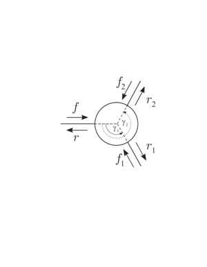
Figure 1: Three-terminal ring with the most general boundary condition. $f$, $r$, etc. denote two-component spinors, the arrows indicate the direction of the corresponding wave number.

As derived in Refs. Földi et al., 2006, Kálmán et al., 2008b, and in the Appendix, if the equations

$$\cos\left(w\pi\right) = 2\cos\left(q\frac{2\pi}{3}\right),$$ (6a)

$$\sin\left(w\pi\right) = \frac{ka}{q}\sin\left(q\frac{2\pi}{3}\right),$$ (6b)

are satisfied simultaneously then the ring polarizes a totally unpolarized input, given by the density matrix $\varrho$, proportional to the identitiy. The polarized spinors exiting at the two outputs

$$\left|\phi_{1}\right>=\begin{pmatrix}-e^{-i\frac{\pi}{3}}\sin\frac{\theta}{2}\\ e^{i\frac{\pi}{3}}\cos\frac{\theta}{2}\end{pmatrix},\quad\left|\phi_{2}\right>=\begin{pmatrix}e^{-i\frac{2\pi}{3}}\cos\frac{\theta}{2}\\ e^{i\frac{2\pi}{3}}\sin\frac{\theta}{2}\end{pmatrix},$$ (7)

are the eigenstates with nonzero eigenvalues $\eta_{n}$ of the output density matrices $\varrho_{n}=\frac{1}{2}\tilde{T}_{n}(\tilde{T}_{n})^{\dagger}$ ($n=1,2$), where $\tilde{T}_{n}$ are given by Eqs. (28) of the Appendix. The corresponding eigenvalues, which describe the transmission probability in the outputs are

$$\eta_{1}=\eta_{2}=\frac{128k^{4}a^{4}q^{2}\sin^{2}\left(q\frac{2\pi}{3}\right)}{\left|\tilde{y}\right|^{2}},$$ (8)

where

$$\tilde{y} = 8q^{3}\left[\cos\left(w\pi\right)+\cos\left(2q\pi\right)\right]-12ikaq^{2}\sin\left(2q\pi\right)$$ (9)

$$+6k^{2}a^{2}q\left[\cos\left(2q\pi\right)-\cos\left(q\frac{2\pi}{3}\right)\right]$$

$$+ik^{3}a^{3}\left[3\sin\left(q\frac{2\pi}{3}\right)-\sin\left(2q\pi\right)\right].$$

If we determine the spinors $\left|\phi_{n}^{0}\right>$ ($n=1,2$) annuled by the transmission matrices $\tilde{T}_{n}\left|\phi_{n}^{0}\right>=0$

$$\left|\phi_{1}^{0}\right>=\begin{pmatrix}\cos\frac{\theta}{2}\\ \sin\frac{\theta}{2}\end{pmatrix},\quad\left|\phi_{2}^{0}\right>=\begin{pmatrix}-\sin\frac{\theta}{2}\\ \cos\frac{\theta}{2}\end{pmatrix},$$ (10)

then it can easily be seen, that if the input state is the $\left|\phi_{1}^{0}\right>$ ($\left|\phi_{2}^{0}\right>$) pure state, then the transmission into output lead 1 (2) will be zero, while the spin direction of the output in lead 2 (1) will be given by $\left|\phi_{2}\right>$ ($\left|\phi_{1}\right>$), i.e.:

$$\left|\phi_{1}^{0}\right> \rightarrow \left\{\begin{array}[]{ll}\left|\phi_{2}\right>\text{in lead {2}}\\ \text{no output in lead {1}}&\end{array}\right.$$ (13)

$$\left|\phi_{2}^{0}\right> \rightarrow \left\{\begin{array}[]{ll}\text{no output in lead {2}}&\\ \left|\phi_{1}\right>\text{in lead {1}}&\end{array}\right.$$ (16)

These –orthogonal– input states are suitable to represent the coin states $\left\{\left|L\right>,\left|R\right>\right\}$ in the QW as they form a basis in the two-dimensional space of the electron spin, and the polarizing three-terminal ring acts on them as the step operator in the QW: if the input spin (coin) state is $\left|\phi_{1}^{0}\right>$ ($\left|\phi_{2}^{0}\right>$) the electron is transmitted into the output lead 2 (1), i.e. the walker ’takes a step to the left (right)’. The change in the spin direction at the outputs given by Eq. (7) means that the states $\left|\phi_{1}\right>$ and $\left|\phi_{2}\right>$ are rotated versions of the two orthogonal inputs $\left|\phi_{2}^{0}\right>$ and $\left|\phi_{1}^{0}\right>$, respectively, where the rotation is around the z-axis by the angle of the given output lead. As we will see in the following, these rotations can be reversed by the application of appropriate rings.

In order for the transformation to be unitary the step-ring also has to be reflectionless, that is the transmission probabilities into the two outputs given by Eq. (8) should be equal to unity, i.e. $\eta_{1}=\eta_{2}=1/2$. It can be easily verified that this condition can be formulated by the following equations

$$k^{2}\!a^{2}\!\sin^{2}\!\left(\!q\frac{2\pi}{3}\!\right)\!\cos\left(\!q\frac{2\pi}{3}\!\right)\!+\!q^{2}\!\left[\cos\left(w\pi\right)\!+\!\cos\left(2q\pi\right)\right]=0,$$ (17a)

$$k^{2}\!a^{2}\!\sin^{3}\!\left(\!q\frac{2\pi}{3}\!\right)\!+\!q^{2}\!\sin\left(2q\pi\right)=0.$$ (17b)

which, for an appropriate combination of the parameters $\left\{a,\omega/\Omega,\gamma_{2}\right\}$ can be satisfied together with Eqs. (6a) and (6b) as can be seen in Fig. 2 for the experimentally feasible range of the parameters.

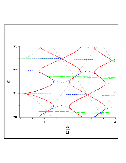
Figure 2: (Color online) Determination of the parameter values corresponding to the step ring: Eqs. (6a) and (6b) are satisfied along the blue (dotted) and grey (dashdotted) lines, respectively, while Eqs. (17a) and (17b) are satisfied along the red (solid) and green (dashed) lines, respectively. At the intersection of these four curves the totally symmetric ($\gamma_{1}=2\pi/3$, $\gamma_{2}=4\pi/3$) three-terminal ring behaves as a perfect polarizing device with practically zero reflection, i.e. as the step ring.

In order to use the same building blocks (i.e. the Hadamard ring and the step ring again) for later steps, the rotations on the basis states introduced by the step ring need to be removed. This can be done eg. by the application of two two-terminal rings which act as $\hat{T}^{\left(1\right)}=U_{2\pi/3}^{-1}$ and $\hat{T}^{\left(2\right)}=U_{4\pi/3}^{-1}$, where

$$U_{\gamma}=\left(\begin{matrix}e^{-i\frac{\gamma}{2}}&0\\ 0&e^{i\frac{\gamma}{2}}\end{matrix}\right).$$ (18)

Although these conditions can be fullfilled if $\gamma=4\pi/3$, and $\gamma=2\pi/3$, respectively, the radius of the rings cannot by made equal to that of the step ring, which does not permit the simple attachment of successive building blocks. We will show in the following section, that three-terminal rings of the same size as the step ring with an appropriate SOI strength, can also rotate the spin states in the desired way, as well as allow of the continuation of the units.

IV Interference at intermediary positions

Clearly, the functional units have to be combined so that the walker can arrive in any intermediate point on the ’line of the walk’ from two directions, i.e., interference phenomena can take place. In order to implement this crucial property of the QW, we use another quantum ring, which is capable of adding the two probabilty amplitudes that both represent the walker at the given point on the ’line of the walk’, as well as rotating the spins back into the basis states $\left|\phi_{1}^{0}\right>$ and $\left|\phi_{2}^{0}\right>$. Now we show, that this can be done with a completely symmetric three-terminal ring which has the same radius as the step ring, and in which the magnitude of the SOI strength is the same, but its direction is opposite.

If two leads of a symmetric, three-terminal ring are considered as inputs and the other terminal as an output (see Fig. 1 with $f=0$), the matrices of the one-input case, given by Eqs. (20) and (21), are enough to handle the problem. Kálmán et al. (2008a) Namely, we can consider the two inputs $f_{i}$ ($i=1,2$) separately, and determine the corresponding matrices. The outputs in each terminal in the superposed problem will consist of contributions from both inputs. Considering $f_{1}$ ($f_{2}$) as the only input, the transmission matrices in the reference frame of $f_{1}$ ($f_{2}$) are the same as those for the input $f$, given by Eqs. (20) and (21). In order to get the contributions to the output spinors ($r,r_{1},r_{2}$) for the input $f_{1}$ ($f_{2}$) in the reference frame of $r$, the matrices need to be rotated by the angle of $\gamma_{1}=2\pi/3$ ($\gamma_{2}=4\pi/3$). Furthermore, since we have considered a propagation of the electron from the left to the right, the symmetric three-terminal ring we want to use to add the two (spin-dependent) probability amplitudes has to be rotated by an angle of $\pi$ with respect to Fig. 1. This means an additional rotation of each matrix by $\pi$.

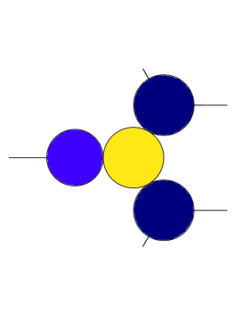
Figure 3: (Color online) The geometry of the functional unit of the scheme, where the rotations introduced by the step ring are removed by symmetric three-terminal rings of the same size as the step ring, but with opposite SOI strength. The colors indicate the value of the SOI strength ($\omega/\Omega$): light blue, yellow and dark blue corresponding to -1, 2.27 and -2.27, respectively. The radius of the Hadamard ring is $a_{H}=0.248$ $\mu$m, while that of the other rings is $a_{S}=0.266$ $\mu$m.

If the radius of the above mentioned ring is the same as that of the step-ring, and the applied SOI strength ($\omega/\Omega$) is of the same magnitude, but opposite direction (in which case the polarization condition given by Eq. (6), and the condition for zero reflection of the input, given by Eq. (17) also hold), then by using Eqs. (28) of the Appendix, it can easily be shown that zero reflection in the two input arms without any transmission from one input lead into the other (i.e. $r_{1}=r_{2}=0$) is automatically guaranteed. Additionally, the probability of transmission from the two inputs into the output is the same, and the coin states $\left|\phi_{1}\right>$ and $\left|\phi_{2}\right>$ are rotated into $\left|\phi_{2}^{0}\right>$ and $\left|\phi_{1}^{0}\right>$, respectively. Hence, such a ring will be able to transform the two inputs into the superposition of the basis states ($\left|\phi_{1}^{0}\right>$ and $\left|\phi_{2}^{0}\right>$) with the same weights.

This ring can also be used for the same purpose as the two-terminal rings mentioned in the previous section. Fig. 3 shows the functional unit of the scheme. The colors of the rings denote the value of the SOI strength, which together with the appropriate radius of the ring, guarantee that no reflection occurs at the inputs. The advantage of using this symmetric three-terminal ring is that it has the same size as the step ring, providing a more symmetrical arrangement for the QW (see Fig. 4). Additionally, measuring currents at the junctions indicated by the short lines in Fig. 3, can be used for determining the functionality of the device: No currents leave the network through these leads under ideal circumstances.

V The proposed scheme

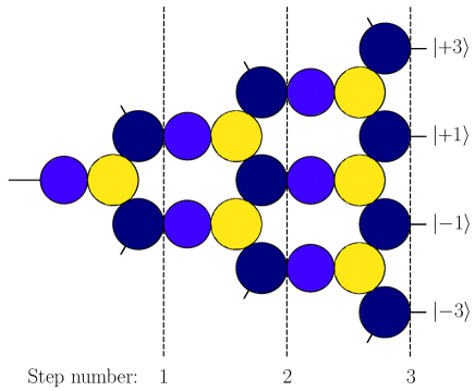
Figure 4: (Color online) The geometry of the device for three steps. The colors and the radii of the rings are the same as in Fig. 3. The vertical dashed lines indicate where the discrete steps take place along the horizontal direction. The vertical direction corresponds to the ’line of the walk’, along which the walk takes place. We have indicated in the vertical direction on the right hand side of the figure the discrete position states of the walker (the electron) on the line after three steps.

Our scheme uses several functional units as building blocks for the implementation of the QW on the line, thus actually it corresponds to a two-dimensional displacement of the walker (the electron). One spatial dimension represents the ’line of the walk’ along which the walk is realized, while the role of the other dimension is twofold. First it is necessary from the technical point of view, it is needed for the transformations (coin-toss, and step) to be made, but it is also related to the discrete time steps of the walk: the number of the functional units increases in this direction, according to the possible positions of the walker that completes increasing number of steps. In other words, the notion of time enters the otherwise time-independent scheme via this spatial direction.

Fig. 4 shows a device capable of implementing three steps of a QW on the line with a Hadamard coin. The colors denote the value of the SOI strength in the rings, which together with the appropriate radius of the ring, guarantee that no reflection occurs at the inputs. For the removal of the rotations of the spins the same symmetric three-terminal ring is used (see Fig. 3) as the one which adds the probability amplitudes at intermediary positions. The vertical dashed lines indicate where the discrete steps take place along the horizontal direction. The vertical direction corresponds to the ’line of the walk’, along which the walk takes place. On the right hand side of the figure we have indicated the discrete position states of the walker (the electron) on the ’line of the walk’ after three steps. As the transmission probabilities are proportional to the value of the current, by measuring the currents on these terminals the distribution characteristic of a QW appears.

VI Conclusion

We have proposed a scheme for the implementation of the coined QW on the line, where the coin is the spin of the electron, quantum rings are used to realize the coin-toss and the step operations, and the shift of the electron in one spatial direction corresponds to the walk along the line.

Let us note that our scheme is based on a one-dimensional model of quantum rings, that assumes single channel ballistic transport. Although spin coherence lengths of 100 and 350 $\mu$m have been found in bulk GaAs Kikkawa and Awschalom (1999) and Si Huang et al. (2007) samples, respectively, the coherence lengths of the orbital wave function are typically two magnitudes shorter, even in modulation doped heterostructures, where the mobility is higher. In the case of InGaAs/InAlAs, the coherence lengths of the orbital wave function are typically in the range of a few microns, Bergsten et al. (2006) which means a severe constrain for our QW scheme. On the other hand, there are samples, where transport is due to many channels in the ring, König et al. (2006) for which our results are not directly applicable. It is beyond the scope of this paper to investigate in detail how phase destroying events affect the functionality of the proposed network, but preliminary results indicate that the functionality can tolerate moderate level of scattering induced errors, thus a few steps of the QW could be implemented.

Our aim was to demonstrate the possibility of a scheme for the QW with semiconductor quantum rings. Further optimization on the number of rings, and the geometry of the network might be possible.

Appendix

For the sake of completeness we present the analytic expressions for the transmission matrices of one-input two- and three-terminal rings, in which Rashba SOI is present. These matrices are obtained by applying Griffith’s boundary conditions Griffith (1953) at the junctions between the incoming lead and the ring, and the outgoing lead(s) and the ring (see Fig. 1), that is, requiring vanishing net spin current density at a certain junction, as well as the continuity of the spinor valued wave functions.

The transmission matrix of a two-terminal ring (see Fig. 1 without lead 2 and $\gamma_{1}=\gamma$) is given by Földi et al. (2005)

$$\hat{T}_{\uparrow\uparrow} = \frac{4ikaq}{\hat{y}}e^{-i\frac{\gamma}{2}}\left(h\cos^{2}\frac{\theta}{2}+h^{\ast}\sin^{2}\frac{\theta}{2}\right),$$

$$\hat{T}_{\uparrow\downarrow} = \frac{4ikaq}{\hat{y}}e^{-i\frac{\gamma}{2}}\sin\frac{\theta}{2}\cos\frac{\theta}{2}\left(h-h^{\ast}\right),$$

$$\hat{T}_{\downarrow\uparrow} = e^{i\gamma}\hat{T}_{\uparrow\downarrow},$$ (19)

$$\hat{T}_{\downarrow\downarrow} = \frac{4ikaq}{\hat{y}}e^{i\frac{\gamma}{2}}\left(h\sin^{2}\frac{\theta}{2}+h^{\ast}\cos^{2}\frac{\theta}{2}\right),$$

where

$$h = e^{i\frac{w}{2}\gamma}\left[\sin\left(q\left(2\pi-\gamma\right)\right)-e^{-iw\pi}\sin\left(q\gamma\right)\right],$$

$$\hat{y} = k^{2}\!a^{2}\!\left[\cos\left(2q\left(\pi\!-\!\gamma\right)\right)\!-\!\cos\left(2q\pi\right)\right]\!+\!4ikaq\sin\left(2q\pi\right)$$

$$-4q^{2}\left[\cos\left(w\pi\right)+\cos\left(2q\pi\right)\right],$$

$$\theta = \arctan\left(-\omega/\Omega\right)$$

with $w=\sqrt{1+\omega^{2}/\Omega^{2}}$, and $q=\sqrt{\left(\omega/\Omega\right)^{2}+k^{2}a^{2}}$.

The transmission matrices of a totally symmetric (i.e. $\gamma_{1}=2\pi/3$ and $\gamma_{2}=4\pi/3$) three-terminal ring, which is shown in Fig. 1 (with $f_{1},f_{2}=0$) are given by Földi et al. (2006); Kálmán et al. (2008b)

$$(\tilde{T}_{1})_{\uparrow\uparrow}\! = \!\frac{8kaq}{\tilde{y}}e^{i\frac{2\pi}{3}}\!\left[\cos^{2}\!\frac{\theta}{2}\!\left(h_{1}+h_{2}\right)\!+\!\sin^{2}\!\frac{\theta}{2}\!\left(h_{1}^{\ast}-h_{2}^{\ast}\right)\right],$$

$$(\tilde{T}_{1})_{\uparrow\downarrow}\! = \!\frac{8kaq}{\tilde{y}}e^{i\frac{2\pi}{3}}\!\sin\!\frac{\theta}{2}\cos\!\frac{\theta}{2}\left[\left(h_{1}+h_{2}\right)\!-\!\left(h_{1}^{\ast}-h_{2}^{\ast}\right)\right],$$

$$(\tilde{T}_{1})_{\downarrow\uparrow}\! = \!e^{-i\frac{4\pi}{3}}(\tilde{T}_{1})_{\uparrow\downarrow},$$ (20)

$$(\tilde{T}_{1})_{\downarrow\downarrow}\! = \!\frac{8kaq}{\tilde{y}}e^{-i\frac{2\pi}{3}}\!\left[\sin^{2}\!\frac{\theta}{2}\!\left(h_{1}+h_{2}\right)\!+\!\cos^{2}\!\frac{\theta}{2}\!\left(h_{1}^{\ast}-h_{2}^{\ast}\right)\right],$$

$$(\tilde{T}_{2})_{\uparrow\uparrow} = (\tilde{T}_{1})_{\downarrow\downarrow},$$

$$(\tilde{T}_{2})_{\uparrow\downarrow} = -(\tilde{T}_{1})_{\downarrow\uparrow},$$

$$(\tilde{T}_{2})_{\downarrow\uparrow} = -(\tilde{T}_{1})_{\uparrow\downarrow},$$ (21)

$$(\tilde{T}_{2})_{\downarrow\downarrow} = (\tilde{T}_{1})_{\uparrow\uparrow},$$

where

$$h_{1} = kae^{iw\frac{\pi}{3}}\sin^{2}\left(q\frac{2\pi}{3}\right),$$ (22)

$$h_{2} = -iq\left[e^{iw\frac{\pi}{3}}\sin\!\left(q\frac{4\pi}{3}\right)\!-\!e^{-iw\frac{2\pi}{3}}\sin\!\left(q\frac{2\pi}{3}\right)\right],$$ (23)

$$\tilde{y} = 8q^{3}\left[\cos\left(w\pi\right)+\cos\left(2q\pi\right)\right]-12ikaq^{2}\sin\left(2q\pi\right)$$ (24)

$$+6k^{2}a^{2}q\left[\cos\left(2q\pi\right)-\cos\left(q\frac{2\pi}{3}\right)\right]$$

$$+ik^{3}a^{3}\left[3\sin\left(q\frac{2\pi}{3}\right)-\sin\left(2q\pi\right)\right].$$

In order for such a ring to polarize a totally unpolarized input that is described by the density matrix $\varrho$ proportional to the identitiy, the output density operators $\varrho_{n}=\tilde{T}_{n}\varrho(\tilde{T}_{n})^{\dagger}$ ($n=1,2$) need to be projectors

$$\varrho_{n}=\frac{1}{2}\tilde{T}_{n}(\tilde{T}_{n})^{\dagger}=\eta_{n}\left|\phi_{n}\right>\left<\phi_{n}\right|,$$ (25)

where the nonnegative numbers $\eta_{n}$ measure the efficiency of the polarizing device. Equation (25) is equivalent to requiring the determinants of $\tilde{T}_{n}(\tilde{T}_{n})^{\dagger}$ to vanish. These determinants are equal, and zero if $h_{1}\pm h_{2}=0$, which, using Eqs. (22) and (23) can be formulated as

$$\cos\left(w\pi\right) = 2\cos\left(q\frac{2\pi}{3}\right),$$ (26)

$$\sin\left(w\pi\right) = \pm\frac{ka}{q}\sin\left(q\frac{2\pi}{3}\right).$$ (27)

If we focus on the case when condition $h_{1}+h_{2}=0$ holds, then the transmission matrices have the simple form

$$\tilde{T}_{1} = \tilde{c}\left(\begin{array}[]{cc}e^{i\frac{2\pi}{3}}\cos^{2}\frac{\theta}{2}&e^{i\frac{2\pi}{3}}\sin\frac{\theta}{2}\cos\frac{\theta}{2}\\ e^{-i\frac{2\pi}{3}}\sin\frac{\theta}{2}\cos\frac{\theta}{2}&e^{-i\frac{2\pi}{3}}\sin^{2}\frac{\theta}{2}\end{array}\right),\quad$$ (28c)

$$\tilde{T}_{2} = \tilde{c}\left(\begin{array}[]{cc}e^{-i\frac{2\pi}{3}}\sin^{2}\frac{\theta}{2}&-e^{-i\frac{2\pi}{3}}\sin\frac{\theta}{2}\cos\frac{\theta}{2}\\ -e^{i\frac{2\pi}{3}}\sin\frac{\theta}{2}\cos\frac{\theta}{2}&e^{i\frac{2\pi}{3}}\cos^{2}\frac{\theta}{2}\end{array}\right),\quad\quad$$ (28f)

where $\tilde{c}=8kaqh_{1}/\tilde{y}$. In the above equations $\theta$, and $\tilde{c}$ are determined by the parameters $\left[ka,\omega/\Omega\right]$ calculated from the polarization condition given by Eq. (6). Using Eqs. (28), the polarized outputs $\left|\phi_{n}\right>$ can easily be determined as the eigenstates of the output density matrices $\varrho_{n}=\frac{1}{2}\tilde{T}_{n}(\tilde{T}_{n})^{\dagger}$ corresponding to the nonzero eigenvalues $\eta_{n}$.

References

- Aharonov et al. (1993) Y. Aharonov, L. Davidovich, and N. Zagury, Phys. Rev. A 48, 1687 (1993).
- Kempe (2003) J. Kempe, Contemp. Phys. 44, 307 (2003).
- Konno (2008) N. Konno, in Quantum Potential Theory, Lecture Notes in Mathematics, Vol. 1954, edited by U. Franz and M. Schurmann (Springer, 2008), pp. 309–452.
- Meyer (1996a) D. Meyer, J. Stat. Phys. 85, 551 (1996a).
- Meyer (1996b) D. Meyer, Phys. Lett. A 223, 337 (1996b).
- Watrous (2001) J. Watrous, J. Comput. Syst. Sci. 62, 376 (2001).
- Farhi and Gutmann (1998) E. Farhi and S. Gutmann, Phys. Rev. A 58, 915 (1998).
- Childs et al. (2002) A. Childs, E. Farhi, and S. Gutmann, Quantum Inf. Process. 1, 35 (2002).
- Kendon (2006) V. Kendon, Philos. Trans. R. Soc. London, Ser. A 364, 3407 (2006).
- Santha (2008) M. Santha, Proceedings of the 5th Theory and Applications of Models of Computation (TAMC08) 4978, 31 (2008).
- Shenvi et al. (2003) N. Shenvi, J. Kempe, and K. B. Whaley, Phys. Rev. A 67, 052307 (2003).
- Travaglione and Milburn (2002) B. C. Travaglione and G. J. Milburn, Phys. Rev. A 65, 032310 (2002).
- Sanders et al. (2003) B. C. Sanders, S. D. Bartlett, B. Tregenna, and P. L. Knight, Phys. Rev. A 67, 042305 (2003).
- Di et al. (2004) T. Di, M. Hillery, and M. S. Zubairy, Phys. Rev. A 70, 032304 (2004).
- Xue et al. (2008) P. Xue, B. C. Sanders, A. Blais, and K. Lalumière, Phys. Rev. A 78, 042334 (2008).
- Eckert et al. (2005) K. Eckert, J. Mompart, G. Birkl, and M. Lewenstein, Phys. Rev. A 72, 012327 (2005).
- Dür et al. (2002) W. Dür, R. Raussendorf, V. M. Kendon, and H.-J. Briegel, Phys. Rev. A 66, 052319 (2002).
- Côté et al. (2006) R. Côté, A. Russell, E. E. Eyler, and P. L. Gould, New J. Phys. 8, 156 (2006).
- (19) Z. Zhao, J. Du, H. Li, T. Yang, Z.-B. Chen, and J.-W. Pan, eprint e-print quant-ph/0212149.
- Hillery et al. (2003) M. Hillery, J. Bergou, and E. Feldman, Phys. Rev. A 68, 032314 (2003).
- Feldman and Hillery (2004) E. Feldman and M. Hillery, Phys. Lett. A 324, 277 (2004).
- Kos̆ík and Buz̆ek (2005) J. Kos̆ík and V. Buz̆ek, Phys. Rev. A 71, 012306 (2005).
- Jeong et al. (2004) H. Jeong, M. Paternostro, and M. S. Kim, Phys. Rev. A 69, 012310 (2004).
- Pathak and Agarwal (2007) P. K. Pathak and G. S. Agarwal, Phys. Rev. A 75, 032351 (2007).
- Chandrashekar (2006) C. M. Chandrashekar, Phys. Rev. A 74, 032307 (2006).
- Li et al. (2008) Y. Li, C. Hang, L. Ma, W. Zhang, and G. Huang, J. Opt. Soc. Am. B 25, C39 (2008).
- Knight et al. (2003) P. L. Knight, E. Roldán, and J. E. Sipe, Phys. Rev. A 68, 020301(R) (2003).
- Du et al. (2003) J. Du, H. Li, X. Xu, M. Shi, J. Wu, X. Zhou, and R. Han, Phys. Rev. A 67, 042316 (2003).
- Perets et al. (2008) H. B. Perets, Y. Lahini, F. Pozzi, M. Sorel, R. Morandotti, and Y. Silberberg, Phys. Rev. Lett. 100, 170506 (2008).
- (30) J. M. Taylor, eprint e-print quant-ph/0708.1484v1.
- (31) K. A. van Hoogdalem and M. Blaauboer, eprint e-print cond-mat.mes-hall/0903.1236v1.
- Manouchehri and Wang (2008) K. Manouchehri and J. B. Wang, J. Phys. A: Math. Gen. 41, 1 (2008).
- Nitta et al. (1999) J. Nitta, F. E. Meijer, and H. Takayanagi, Appl. Phys. Lett. 75, 695 (1999).
- Bergsten et al. (2006) T. Bergsten, T. Kobayashi, Y. Sekine, and J. Nitta, Phys. Rev. Lett. 97, 196803 (2006).
- Nitta and Bergsten (2007) J. Nitta and T. Bergsten, New J. Phys. 9, 341 (2007).
- König et al. (2006) M. König, A. Tschetschetkin, E. M. Hankiewicz, J. Sinova, V. Hock, V. Daumer, M. Schäfer, C. R. Becker, H. Buhmann, and L. W. Molenkamp, Phys. Rev. Lett. 96, 076804 (2006).
- Rashba (1960) E. I. Rashba, Sov. Phys. Solid State 2, 1109 (1960).
- Fabian et al. (2007) J. Fabian, A. Matos-Abiague, C. Ertler, P. Stano, and I. Žutić, Acta Physica Slovaca 57, 565 (2007).
- Nitta et al. (1997) J. Nitta, T. Akazaki, H. Takayanagi, and T. Enoki, Phys. Rev. Lett. 78, 1335 (1997).
- Grundler (2000) D. Grundler, Phys. Rev. Lett. 84, 6074 (2000).
- Awschalom et al. (2002) D. D. Awschalom, D. Loss, and N. Samarth, Semiconductor Spintronics and Quantum Computation (Springer, Berlin, 2002).
- Földi et al. (2005) P. Földi, B. Molnár, M. G. Benedict, and F. M. Peeters, Phys. Rev. B 71, 033309 (2005).
- Földi et al. (2006) P. Földi, O. Kálmán, M. G. Benedict, and F. M. Peeters, Phys. Rev. B 73, 155325 (2006).
- Kálmán et al. (2008a) O. Kálmán, P. Földi, M. G. Benedict, and F. M. Peeters, Phys. Rev. B 78, 125306 (2008a).
- Földi et al. (2008) P. Földi, O. Kálmán, M. G. Benedict, and F. M. Peeters, Nano Letters 8, 2556 (2008).
- Bellucci and Onorato (2008) S. Bellucci and P. Onorato, Phys. Rev. B 78, 235312 (2008).
- Molnár et al. (2004) B. Molnár, F. M. Peeters, and P. Vasilopoulos, Phys. Rev. B 69, 155335 (2004).
- Meijer et al. (2002) F. E. Meijer, A. F. Morpurgo, and T. M. Klapwijk, Phys. Rev. B 66, 033107 (2002).
- Griffith (1953) S. Griffith, Trans. Faraday Soc. 49, 345 (1953).
- Büttiker et al. (1984) M. Büttiker, Y. Imry, and M. Y. Azbel, Phys. Rev. A 30, 1982 (1984).
- Voo (2009) K.-K. Voo, Physica E 41, 441 (2009).
- Kálmán et al. (2008b) O. Kálmán, P. Földi, M. G. Benedict, and F. M. Peeters, Physica E 40, 567 (2008b).
- Kikkawa and Awschalom (1999) J. M. Kikkawa and D. D. Awschalom, Nature 397, 139 (1999).
- Huang et al. (2007) B. Huang, D. J. Monsma, and I. Appelbaum, Phys. Rev. Lett. 99, 177209 (2007).