Wigner’s Theorem
and geometry of extreme positive maps
Abstract
We consider transformation maps on the space of states which are symmetries in the sense of Wigner. By virtue of the convex nature of the space of states, the set of these maps has a convex structure. We investigate the possibility of a complete characterization of extreme maps of this convex body to be able to contribute to the classification of positive maps. Our study provides a variant of Wigner’s theorem originally proved for ray transformations in Hilbert spaces.
MSC 2000: (Primary 52A20), (Secondary 81Q70).
PACS: 02.40.Ft, 03.65.Fd
Key words: density states, convex sets, extreme points, positive maps, Wigner’s theorem
1 Introduction
Symmetries play a very important role in physics, as it has been stressed by Wigner on several occasions [1, 2, 3]. The way symmetries are realized depends on the theory under consideration and more specifically, according to Felix Klein, on the corresponding geometric structure of the carrier space, these are ‘kinematical’ rather than ‘dynamical’ symmetries. It is well known that any description of physical systems requires the consideration of states and observables along with a pairing among them providing a real number with a computable probability [4]. In the Schrödinger-Dirac description of Quantum Mechanics one associates a Hilbert space with a quantum system, states are identified with rays of this space and observables are a derived concept – they are identified with self-adjoint operators, while symmetries are defined to be bijections among rays which preserve probability transitions.
In the -algebraic approach to Quantum Mechanics, originated from the Heisenberg picture, observables are identified with real elements of this -algebra, while states are a derived concept – they are identified with positive normalized functionals on the space of observables. The space of observables carries the structure of a Jordan algebra and this was the point of view of Kadison to define symmetries as Jordan-algebra isomorphisms [5, 6]. -algebras are quite convenient to deal with the description of composite systems, the dual space of states turns out to have a rather involved geometrical structure. In particular, to take into account the distinction between separable and entangled states on the space of states, one is obliged to give up linear superposition in favor of convex combinations. This change of perspective introduces highly nontrivial problems, specific to the ‘convex setting’. As shown elsewhere [7], in finite dimensions the space of states turns out to be a stratified manifold with faces of various dimensions.
The aim of this paper is to deal with symmetries as those transformations on the space of states which are appropriate for its geometrical structure. In doing this we end up with yet another variant of the celebrated Wigner’s theorem on the realization of symmetries as unitary or antiunitary transformations on the Hilbert space. The literature on this theorem, which is also available on text books [8, 9] in addition to the famous book by Wigner [10], is huge. We limit ourselves to a partial list trying to give a sampling of the various approaches which have been taken in the years [11, 12, 13, 14, 15, 16, 17, 18, 19].
The paper is organized in the following way: in Section 2 we give a short geometrical description of the set of density states in a finite-dimensional Hilbert space. Density states form a convex body in the space of Hermitian operators. The set of affine maps which map a convex set into itself, called simply positive maps, is also a convex set in the space of affine maps. Characterization of positive maps, e.g. by identifying the extremal ones, i.e. maps which can not be decomposed into a nontrivial convex combination of other positive maps, can lead to a useful description of the underlying set . Finding extreme points of such maps is, however, a difficult task, even if we know explicitly the extreme points of . In Section 3 we discuss and give examples of positive maps for which their extremality can be established upon analyzing the number of extreme points in the image. In Section 4 we connect the obtained results to the Wigner’s theorem expressed in terms of positive maps which are bijective on pure states. Sections 5 and 6 are devoted to completely positive maps. In particular, we show again how the number of extreme points in their image establishes their form and extremality. We conclude with Section 7 containing illustrative examples of extreme positive and completely positive maps in low dimensions.
2 Density states
Let be a finite-dimensional Hilbert space, , and let be the space of complex linear operators on . The space is canonically a Hilbert space itself with the Hermitian product . As in [7], we shall treat the real linear space of Hermitian operators on as the dual space, , of the Lie algebra (of antihermitian operators), , of the unitary group . We have the obvious decomposition into real subspaces with a natural pairing between and given by
| (1) |
and a scalar product induced on by the Hermitian product and given by
| (2) |
We denote with the corresponding norm.
The coadjoint action of on reads
| (3) |
We denote by the space of positive semi-definite operators from , i.e. of those which can be written in the form for a certain . It is a cone, since it is invariant with respect to the homotheties by with . The set of density states is distinguished in the cone by the equation , so we will regard and as embedded in .
The space is a convex set in the affine hyperplane in , determined by the equation . The model vector space for is therefore canonically identified with the space of Hermitian operators with trace . The space of affine maps of can be canonically identified with the space of these linear maps which preserve the trace.
It is known that the set of extreme points of coincides with the set of pure states, i.e. the set of one-dimensional orthogonal projectors , and that every element of is a convex combination of points from . The space of pure states can be identified with the complex projective space via the projection
which identifies the points of the orbits of the -group action by complex homotheties.
If we choose an orthonormal basis in , we can identify with the real vector space of Hermitian matrices, with the affine space of Hermitian matrices with trace 1, with the group of unitary matrices, with - the convex body of density matrices, etc. Recall that the dimension of is and the dimension of is .
Almost all above can be repeated in the case when is infinite-dimensional if we assume that all the operators in question, i.e. operators from and are Hilbert-Schmidt operators (see [20]). The positive semi-definite operators then, being of the form , are trace-class (nuclear) operators, so density states are trace-class operators with trace 1. There are some obvious minor differences with respect to finite dimensions: for instance, the convex set of density states is the closed convex hull of the set of pure states, rather than just the convex hull, etc.
3 Positive maps of convex sets
If is a convex set in a locally convex topological vector space , then the set of those continuous linear maps which map into is a convex set in the (real) vector space of all continuous linear maps from into . We will refer to elements of as to linear -positive maps, or simply to linear positive maps, if is determined.
If is compact, then, due to the Krein-Milman Theorem, it is the closed convex hull of the set of its extreme points (points which are not interior points of intervals included in ), . In this sense, compact convex sets are completely determined by their extreme points.
However, it should be made clear from the beginning that the concepts of convex set, positive map, etc., are taken from the affine rather than linear algebra and geometry. In an affine space , one can subtract points, , to get vectors of the model vector space , or add a vector to a point, , to get another point, but there is no distinguished point that serves as the origin. More generally, in affine spaces we can take affine combinations of points, i.e. combinations such that . If all are non-negative the corresponding affine combination is just a convex combination. We say that points are affinely independent if none is an affine combination of the others. This is the same as to say that are linearly independent vectors.
Convex sets in our approach will live in affine spaces. In this sense the Krein-Milman Theorem tells us something about compact convex sets in affine spaces modeled on locally convex linear spaces.
One can think that the problem is artificial, since by choosing a point in an affine space as the origin we end up in the model vector space. However, choosing a point is an additional information put into the scheme which changes our setting. The situation is like in a gauge theory, where we can fix a gauge. But a fixed gauge has, in general, no physical interpretation, so we rather try to use gauge-invariant objects.
The second instance of affine space presence is the fact that in many situations, even when we work in a true linear space, it makes much more sense to admit that positive maps are affine. Note that affine maps on an affine hyperspace of a linear space come exactly from linear maps in which preserve . On the other hand, every affine space (or even affine bundle) can be canonically embedded in a linear space (vector bundle) as an affine hyperspace (affine hyperbundle). We refer to [21, 22] for the corresponding theory with interesting applications to frame-independent formulations of some problems in Analytical Mechanics.
Definition 1.
(a) Let be a real affine space modeled on a locally convex topological real vector space , . We say that a map is an affine map if there is a continuous linear map such that for any and any , we have , where is the natural action of on . The space of affine maps from to will be denoted by . If , for the space of affine maps on , i.e. for we will write shortly .
(b) Let be the space of all affine maps on and let be a convex set in . By positive maps on (or simply positive maps if there is no ambiguity about ) we understand these affine maps which map into . The set of all positive maps on will be denoted by .
(c) By a convex body we will understand a compact convex set with non-empty interior in a finite-dimensional Euclidean affine space .
Note that the set of density states for quantum systems with a finite number of levels is an example of a convex body, as it is canonically embedded in the Euclidean affine space of Hermitian operators with trace 1 – an affine hyperspace of .
It is easy to see that for a compact convex set in a finite-dimensional affine space the closed convex hull is just the convex hull if only is closed, and that the convex set of positive maps is again a compact convex set, this time in . Note that is canonically an affine space modeled on the vector space of affine maps from into . Moreover, if is just a vector space, , the space is a vector space with a canonical decomposition , due to the fact that we can write any affine map uniquely in the form for some and .
3.1 Fix-extreme positive maps
In general it is not easy to find extreme points of the convex set of positive maps , even if extreme points of the convex body are explicitly known. This is exactly the case of the convex bodies of positive maps in Quantum Mechanics.
On the other hand, extremality of some positive maps can be established relatively easy in the case of maps with many extreme points in the image, as each extreme point in the image fixes partially the map. This is based on the observation that, for , if is the image for some , then for any of a decomposition into a convex combination of . Indeed, as is a decomposition of the extreme point into a convex combination of points , then . This immediately implies the following.
Theorem 1.
Let be a compact convex set in an -dimensional real affine space. If a positive map has affinely independent extreme points in the image of , then the map is extreme positive, .
Proof.
Let , , be such that are extreme and affinely independent and assume that we have a decomposition for certain and . According to the observation preceding the above theorem, for all . But an affine map from a -dimensional affine space is completely determined by its values on affinely independent points, so . ∎
The extreme positive maps described in the above theorem (with affinely independent extreme points in the image ) will be called fix-extreme positive maps.
Corollary 1.
For any convex body a positive map which has all extreme points in is extreme positive. In particular, the identity map is always an extreme positive map.
3.2 Example: the closed unit ball in
Theorem 2.
Fix-extreme positive maps of unit balls in Euclidean vector spaces are orthogonal transformations.
The proof of the above theorem will be based on the following lemma.
Lemma 1.
If the function ,
where and , , has on the unit sphere local maxima at some affinely independent points , then is constant on . In particular, and .
Proof.
We will use the method of Lagrange multipliers and consider the function
Since , , are critical points of , when restricted to the sphere, the coordinates of each solve the system of equations
| (4) | |||||
Moreover, as at we have local maxima, the second derivative of must be non-positive definite that yields for all . We can assume that , so .
Assume first that . Then,
| (5) |
and
should be equal to 1. But the function is monotone with respect to , so there is at most one solution of (4) with . It must be therefore at least additional solutions with . Let be the number of the biggest , i.e. . We get easily from (4) that
| (6) |
Hence if then is constantly on the sphere. It suffices to show now that is not possible. Indeed, if is a solution of (4) with , we get
so we can have, together with the solution (5) corresponding to , an affinely independent set of solutions only if . But then, due to (6), the solution (5) must be
| (7) |
so and reduces to
and
| (8) |
On the other hand, the solutions corresponding to must be of the form
so that we have solutions additional to (7) only if
| (9) |
But, as , the latter contradicts (8):
∎
Now we can prove Theorem 2.
Proof.
Let be the unit ball in an -dimensional Euclidean vector space . Let us make an identification of with with the standard Euclidean norm
Let be a fix-extreme positive map of , i.e. is an affine map, , where is a linear map of such that and has affinely independent points in the unit sphere . Of course, we can assume that are extreme points of , so they lie on the sphere as well. In particular the map (matrix) is invertible.
Now we can apply the singular value decomposition to the matrix in order to write it in the form , where are orthogonal matrices and is a diagonal matrix with positive entries on the diagonal. Since we can write
where , and since the orthogonal maps preserve and , the map has the same properties as : it is a positive map of , and has affinely independent points on the unit sphere , where are points of the sphere, . This means that the function
reduced to the unit sphere takes at local maxima. Applying the above lemma we conclude that and is constant on the sphere, so that maps the unit sphere into the unit sphere. Hence, and is orthogonal. ∎
3.3 Example: an extreme map on the plane fixing two extreme points
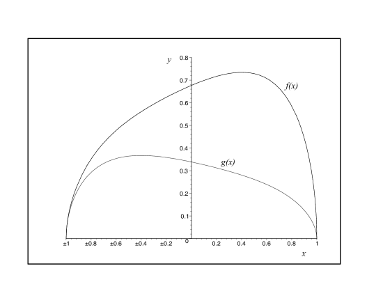
In the present section we want to present a simple example of an extreme map in two dimensions which is a bijection on its two extreme points. To this end let us consider the function on the interval ,
| (10) |
The function is concave, hence the subset of the plane bounded by its graph and the interval is convex. Let us perform a linear transformation of the plane,
| (11) |
Under this transformation is transformed into the set bounded by and the graph of
| (12) |
i.e.
| (13) |
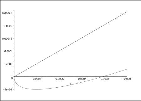
Since for , we have . Moreover is a bijection on two extremal points, and , of . Observe also that is an extreme mapping in the sense that for an arbitrary there is such that , i.e. the linear transformation
| (14) |
does not map into .
The above described properties of and can be established by straightforward calculations. Below we illustrate them in Figures 1-3.

4 Positive maps bijective on pure states - a version of Wigner’s Theorem
Before we formulate a version of the Wigner’s Theorem [14] let us comment on complex antilinear and antiunitary maps in a Hilbert space. A map we call antilinear if , where denotes the complex conjugation of . An antilinear map we call antiunitary if for all . The adjoint of an antilinear map is an antilinear map defined via the identity
Any linear (antilinear) map induces a linear (resp., antilinear) map which on one-dimensional maps takes the form . For linear we can easily represent the map as , while with antilinear maps the situation is a little bit more complicated.
If an orthonormal basis is chosen then in the Hilbert space we can define a complex conjugation
Instead of we will write simply . It is clear that . If is a complex linear map then is antilinear and vice versa. Since any continuous complex linear (antilinear) map is represented by a (possibly infinite) matrix , where , also the transposition is well defined:
and we extend it to the whole by complex linearity (antilinearity). For linear the adjoint map can be then written as
so that for linear Hermitian . If is antilinear then is linear, so
But, as easily seen,
so that, for Hermitian ,
| (15) |
The Wigner’s Theorem (compare with [14]) can be now formulated as follows.
Theorem 3.
Let be a bijection of pure states in a Hilbert space preserving the transition probabilities
| (16) |
Then, there is a unitary such that
| (17) |
or
| (18) |
where is the transposition associated with a choice of an orthonormal basis in .
The standard versions of Wigner’s Theorem usually consider (unit) vectors of the Hilbert space rather than pure states. But if are unit vectors representing pure states and , respectively, then
so that preserving is the same as preserving . Moreover, any unitary (or antiunitary) action in the Hilbert space, , induces on pure states the action (17) or (18). We will call the maps (17) and (18) defined on pure states or on Wigner maps. The Wigner maps on can be abstractly characterized as follows.
Theorem 4.
A linear map is a Wigner map if and only if it is positive and orthogonal.
Proof.
The Wigner maps are clearly positive and orthogonal, so let us assume that has these properties. For all Hermitian we have therefore (16) and we know that is positive semi-definite if is. The map is orthogonal, therefore invertible, and its inverse is orthogonal as well. Let us observe that is also a positive map. Take a pure state and suppose that has the spectral decomposition into a difference of positive semi-definite operators which are orthogonal, . Then is a difference of orthogonal positive semi-definite operators and, as is a pure state, (thus ) must be 0. A similar argument shows that the image of any pure state is a positive semi-definite operator which is not decomposable into a sum of orthogonal positive semi-definite operators, so is a pure state up to a constant factor. Since
this factor equals 1 and we conclude that induces a bijection on pure states. ∎
We will now prove a theorem which extends Wigner’s Theorem and which relates it to the problem of extreme positive maps.
Let be the linear subspace of consisting of Hermitian finite-rank operators. For we say that a map is affine if is the restriction to of a trace-preserving linear map from the linear span of in into the linear span of in , .
Theorem 5.
Let be a bijective map. The following are equivalent:
-
(a)
is affine;
-
(b)
preserves transition probabilities between pure states;
-
(c)
is a Wigner map.
If any (or all) of these cases is satisfied, there is a unique continuous affine extension of which is extreme positive, .
Proof.
. Since is spanned by the set of pure states, let be the (unique) linear trace-preserving map on the space of finite-rank Hermitian operators inducing on . Since maps convex combinations into convex combinations, maps finite-rank density states into finite-rank density states, so is a positive map. We will prove that is a linear isomorphism on . This follows from the fact that preserves the rank, i.e. induces a bijection on for each .
To see the latter let us remark that the rank, , of is defined as a minimal number of pure states whose linear combination is , so that, as is linear and is a bijection on pure states, . Conversely, if is of rank , then it is a convex combination of some pure states , thus the image by of a convex combination of pure states . This shows that . The linear map induces a bijection on , so assume inductively that it induces a bijection on for . Let now be of rank , , with the spectral decomposition , with , , and being pairwise orthogonal pure states, , . We must show that the rank of is .
Suppose the contrary. Hence, according to the inductive assumption, is of rank . As , where , thus is of rank , the image of , thus belongs to the image of . Consider the spectral decomposition , with , , and being pairwise orthogonal pure states, , . Let (resp., ) be the subspace in spanned by the vectors (resp., ) and let (resp., ) be the set of all pure states of (resp., ), i.e. these pure states from which are represented by unit vectors from (resp., ). It is now clear that . Note that pure states from can be characterized as such pure states which added to do not change the rank, . According to the inductive assumption this implies that as well, but
which is a contradiction.
Since we know now that induces bijections on each , , it is easy to conclude that it is a rank-preserving isomorphism, so that is also a positive map. Indeed, as spans , it is clearly ”onto”. It is also injective, since , where and are density states of finite ranks, implies ( is positive) that , thus , as preserves the rank of density states.
To finish the proof, we will need the following lemma.
Lemma 2.
Let be a density state of a finite rank . Then the square of the Hilbert-Schmidt norm can be characterized as the maximum of the expressions over all decompositions of as a convex combination of pure states . This maximum is associated with the spectral decomposition.
Proof.
The above lemma implies that the map preserves the Hilbert-Schmidt norm of density states. Indeed, if we use the spectral decomposition to write as a convex combination of pure states, then can be expressed as a convex combination of pure states with the same coefficients, so that . But we can apply the above consideration to instead of and get for any density state of rank , in particular for . We get therefore .
Let us now take two pure states and consider . Since, according to (19),
and
we have
thus
so preserves transition probabilities between pure states.
is the Wigner’s Theorem.
is obvious.
Moreover, has an obvious unique continuous extension , or . Since is positive and has all extreme points in its image, it is extreme positive according to the obvious infinite-dimensional version of Corollary 1. ∎
If the dimension of the Hilbert space is , then the dimension of the affine space of Hermitian operators with trace 1 equals and we know from the general theory (Theorem 1) that a positive map possessing pure states in the image of is extreme positive (we called such positive maps fix-extreme). We finish this section with the following conjecture motivated by Theorem 2.
Conjecture 1.
Any fix-extreme positive map is a Wigner map.
5 Completely positive maps acting on pure states
A linear map is called completely positive (CP) if , where is the algebra of complex matrices, is positivity-preserving for all . It was shown by Choi [24] and Kraus [25] that each CP map admits a representation in the so called Kraus form
| (22) |
where are operators acting on .
Definition 2.
We say that a CP operator (22) acting on Hermitian operators of a Hilbert space is extreme if any decomposition, , into a sum of CP operators is irrelevant, i.e. all the operators are proportional to , , for some . In particular, all operators are proportional and can be written as a single Kraus operator
Not to deal with the cone of CP operators but rather with a compact convex set (if the dimension of is finite), one has to put certain normalization condition. We can try to use, for instance, the trace of a CP operator (22) as a linear operator on the complex vector space which is the same as the trace of (22) as an operator on the real vector space of Hermitian operators.
Theorem 6.
If is a CP operator in the form (22) then
| (23) |
Proof.
It suffices to prove (23) for a single Kraus map . Choose an orthonormal basis in and write in this basis as a complex matrix . As an orthonormal basis in we can take . We have
∎
As we can see, the trace can vanish for non-zero CP operators which makes the normalization by trace impossible. There is, however, another possibility of normalizing CP operators provided by the Jamiołkowski isomorphism [26]
| (24) |
The Jamiołkowski isomorphism maps the operator into the rank-one operator . In particular, CP operators correspond, via the Jamiołkowski isomorphism , to positive semi-definite operators on (see, for instance, [20]). Any Kraus operator corresponds to the one dimensional Hermitian operator . The spectral decomposition of results in the decomposition (22) with being mutually orthogonal with respect to the Hilbert-Schmidt product in . Such a decomposition of a CP operator we will call a spectral decomposition. We will call a CP operator normalized if it corresponds, via the Jamiołkowski isomorphism, to a trace-one operator. If (22) is a spectral decomposition of a CP operator, then it is normalized if
We will call the spectral trace of a CP operator . The spectral trace is greater or equal to 0 and equals 0 only if . The convex set of normalized CP operators on we will denote by . It is clear that extreme points in are exactly single normalized Kraus maps.
From now on we assume the Hilbert space to be of a finite dimension .
Recall that on the space of Hermitian operators on we have a canonical scalar product and that denotes the cone of positive semi-definite operators. We will call elements , , of to be in general position if for any non-zero we cannot find of them which are orthogonal to . If are of rank-one, , where , this simply means that any vectors of form a linear basis in .
Theorem 7.
The following statements are equivalent:
-
(a) is invertible and is a CP operator.
-
(b) is invertible and extreme, i.e.
with - invertible.
-
(c) For any set of pure states in general position, are operators of rank one in general position.
-
(d) In the image there are rank-one operators in general position.
-
(e) There exists a set of pure states in general position such that are operators of rank one in general position.
Proof.
(a)(b). It was proven in [27] (Theorem 7).
(b)(c). If then , hence maps pure states into rank-one operators, and , being invertible, preserves all linear independencies.
(c)(d) - trivial.
(d)(e). Let be positive semi-definite operators such that , , are rank-one operators in general position. First, let us remark that we can assume that are density states, since proportionality plays no role here. Second, we can assume further that they are pure. Indeed, if is a state with the spectral decomposition into a convex combination of pure states and if is rank-one positive semi-definite operator, then is a convex combination of rank-one positive semi-definite operators , so is positively proportional to for all , since pure states are extreme points in the convex body of all states. By a similar argument, all states , , are proportional to , say , where, of course, .
Let us write , , , for some vectors , . We claim that the states are in general position, i.e. any among the vectors are linearly independent.
For, assume the contrary, i.e. that, say , are linearly dependent. Hence, one of the vectors, say , can be written as a linear combination . Since is proportional to , the vector is proportional to for . In particular, all the vectors with and , belong to the linear span of the vectors . Therefore
Since is proportional to , and are linearly independent, we have for all . But this contradicts the property , i.e. .
(e)(a). Put , for some , . Since is of rank one, all the positive semi-definite operators of its decomposition
must be proportional to , . This, in turn, means that are proportional to ,
As any vectors of are linearly independent, all the coefficients of the decomposition
are non-zero, . Since
are proportional to and has a decomposition into a linear combination of linearly independent , the vector must be proportional to . In consequence, it means that the operators are proportional to the operator uniquely defined by the conditions
Hence
for some and, clearly, . ∎
Remark 2.
It is not enough to take only pure states . Let us take, for example, diagonal, , , and not proportional. If now , we have an infinite set of pure states that are mapped to rank-one operators and any of them are not in general position, but is not extreme.
Corollary 2.
If a CP operator
| (25) |
is trace-preserving (resp., unity-preserving) and such that the image of density states contains pure states in general position, then is unitary, .
Proof.
It is enough to make use of Theorem 7 and observe that trace-preserving (unity-preserving) yields (resp., ), so is unitary.
∎
6 Extreme bistochastic CP maps
Extreme unity-preserving CP maps have been described by Man-Duen Choi [24]. We can reformulate his result as follows.
Theorem 8.
Let (resp., ) be the convex body of normalized unity-preserving (resp. trace-preserving) CP maps on . Then (resp. ), with the spectral decomposition
| (26) |
is extreme if and only if the operators (resp., ) are linearly independent in .
Proof.
We will sketch a proof making use of the Jamiołkowski isomorphism (24) which associates with the CP map (26) the Hermitian operator
on . Extreme normalized CP operators correspond therefore, via the Jamiołkowski isomorphism, to pure states on the Hilbert space . On the space of Hermitian operators acting on the Hilbert space , in turn, we can define two canonical -linear maps which associate with rank-one operators the operators and , respectively. The unity-preserving CP operators correspond therefore to Hermitian operators constrained by the equations . The corresponding extreme points need not be pure states. It suffices that the level sets of of the linear constraint are transversal to the face of the point, i.e. the function has the trivial kernel on the tangent space of the face at . But this tangent space is known (see e.g. [7, 27]) to consists of all Hermitian operators with the range equal to the range of , i.e. the operators of the form , where is a Hermitian matrix. Hence is extremal in if and only if
| (27) |
for all Hermitian . As we can decompose any operator into the sum of a Hermitian and an antihermitian ones, we can rewrite (27) in instead of using an arbitrary complex matrix . This is nothing but the complex linear independence of the operators in . For trace-preserving CP operators the reasoning is identical with the function replacing . ∎
The maps from are sometimes called bistochastic. The above understanding of the Choi’s result gives us easily a characterization of extreme bistochastic maps.
Theorem 9.
A bistochastic map with the spectral decomposition
is extreme if and only if the operators are linearly independent in .
Proof.
The proof is analogous to the above one with the difference that our constraint function is now
The condition (27) is therefore replaced by the condition
We can rewrite it as
and pass to an arbitrary complex like before. ∎
7 Examples
Let us illustrate some of the previous reasonings and results in the simplest cases of maps on states on two- and three-dimensional spaces. In the following subsection we show three examples of extreme maps: a generic one possessing exactly two pure states in its image, a non-generic one with only one pure state in the image, and an extreme map having a continuous family of pure states in the image. The last one, according to Theorem 2, is not completely positive but a merely positive extreme map. Note that these cases have been considered also in [29].
In the second subsection we give an example of an extreme completely positive map acting on which does not have any pure state in its image. Such a situation is impossible for maps acting on qubits (i.e. maps on ).
7.1 Extreme completely positive, positive, stochastic and bistochastic maps for
A state on can be parameterized by a unit vector
| (28) |
where
| (29) |
A positive trace-preserving map
| (30) |
is thus determined (up to rotations which are irrelevant from the point of view of this paper) by four parameters , such that
| (31) |
The parameters must fulfil particular conditions to ensure the positivity of the map (see [28], [29] for details).
The image of the unit sphere under (30) is the ellipsoid
| (32) |
Obviously, for a positive map (30) the ellipsoid is inside the unit sphere. For extreme maps it has to have points on its surface common with the surface of the unit sphere (i.e. some pure states are mapped into pure states). For extreme CP maps two possibilities occur [29]:
-
1.
, , , , . In this case the ellipsoid (32) has three different axes and it touches the unit sphere at two points (see Fig. 4).
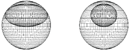
Figure 4: An extreme CP map having exactly two pure states in the image. Projections along two perpendicular axes. -
2.
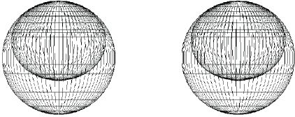
Figure 5: An extreme CP map having exactly one pure state in the image. Projections along two perpendicular axes. -
3.
Geometrically it is obvious that without upsetting the extremality of the map we can make the ellipsoid (32) touching the unit sphere along a full circle (see Fig. 6). In this case
For the map is definitely not a unitary one (its image is a proper subset of the unit sphere) and in its image there are more than 3 pure states (in fact the whole circle of states at which the ellipsoid touches the unit sphere). From Theorem 2 it follows thus that the map cannot be a completely positive one. Indeed, for the chosen values of , and the map is an extreme positive [23]. The fact that it is not completely positive can be checked independently by finding that its image under the Jamiołkowski isomorphism [26] is not positive semi-definite.
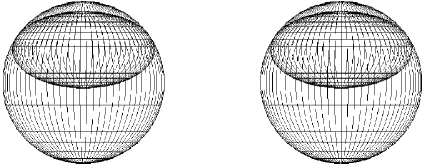
Figure 6: An extreme positive map having a continuous family of pure states in its image. Projections along two perpendicular axes.
7.2 An extreme completely positive map having no pure states in its image
Let us consider a CP map on defined by the following Kraus operators
| (33) |
A straightforward calculation gives .
For the matrices form a basis in the space of matrices, hence it is also true for small . The map is thus an extreme CP map (theorem 8). For there is no such that for some and , hence does not send any pure state into a pure one.
8 Acknowledgements
We thank G. Esposito for reading the manuscript and making useful suggestions. M. K. acknowledges the support by the LFPPI Network financed by the Polish Ministry of Science and Higher Education and the EU Program SCALA (IST-2004-015714).
References
- [1] E. P. Wigner. Invariance in physical theory. Proceedings of the American Philosophical Society, 3:521–526, 1949.
- [2] E. P. Wigner. Events, laws of nature, and invariance principles. Science, 145(3636):995–999, 1964. Nobel Lecture, December 12, 1963.
- [3] R. M. F. Houtappel, H. Van Dam, and E. P. Wigner. The conceptual basis and use of the geometric invariance principles. Rev. Mod. Phys., 37(4):595–632, Oct 1965.
- [4] G. W. Mackey. Mathematical foundations of quantum mechanics. Benjamin, New York, 1963.
- [5] R. V. Kadison. Isometries of operator algebras. Ann. Math., 54:325–338, 1951.
- [6] R. V. Kadison. Transformations of states in operator theory and dynamics. Topology, 3(2):177–198, 1965.
- [7] J. Grabowski, M. Kuś, and G. Marmo. Geometry of quantum systems: density states and entanglement. J. Phys. A: Math. Gen., 38:10217–10244, 2005.
- [8] K. Gottfried and T. M. Yan. Quantum mechanics: fundamentals. Springer, New York, 2004.
- [9] G. Esposito, G. Marmo, and G. Sudarshan. From classical to quantum mechanics: an introduction to the formalism, foundations and applications. Cambridge University Press, Cambridge, 2004.
- [10] E. P. Wigner. Group theory. Academic Press, New York, 1959.
- [11] R. Hagedorn. Note on symmetry operations in quantum mechanics. Nuovo Cimento, 12:73–86, 1959.
- [12] J. S. Lomont and P. Mendelson. The Wigner unitarity-antiunitarity theorem. Ann. Math., 78(3):548–559, 1963.
- [13] L. O’Raifeartaigh and G. Rasche. Probability-conserving transformations and superselection rules in quantum theory. Ann. Phys. (NY), 25:155–173, 1963.
- [14] V. Bargmann. Note on Wigner’s theorem on symmetry operations. J. Math. Phys., 5:862–868, 1964.
- [15] J. E. Roberts and G. Roepstorff. Some basic concepts of algebraic quantum theory. Comm. Math. Phys., 11(4):321–338, 1969.
- [16] W. Hunziker. A note on symmetry operations in quantum mechanics. Helv. Phys. Acta, 45(2):233–236, 1972.
- [17] L. Bracci, G. Morchio, and F. Strocchi. Wigner’s theorem on symmetries in indefinite metric spaces. Comm. Math. Phys., 41(3):289–299, 1975.
- [18] J. Samuel. The geometric phase and ray space isometries. Pramana J. Physics, 48(5):959–967, 1997.
- [19] G. Cassinelli, E. De Vito, P. J. Lahti, and A. Levrero. Symmetry groups in quantum mechanics and the theorem of wigner on the symmetry transformations. Reviews in Mathematical Physics, 9(8):921–942, 1997.
- [20] J. Grabowski, M. Kuś, and G. Marmo. On the relation between states and maps in infinite dimensions. Open Sys. Information Dyn., 14:355–370, 2007.
- [21] K. Grabowska, J. Grabowski, and P. Urbański. AV-differential geometry: Poisson and jacobi structures. J. Geom. Phys., 52:398–446, 2004.
- [22] K. Grabowska, J. Grabowski, and P. Urbański. AV-differential geometry: Euler-lagrange equations. J. Geom. Phys., 57:1984–1998, 2007.
- [23] V. Gorini and E. C. G. Sudarshan. Extreme affine transformations. Commun. Math. Phys., 46:43–52, 1976.
- [24] M. D. Choi. Completely positive linear maps on complex matrices. Linear Alg. Appl., 10:285–290, 1975.
- [25] K. Kraus. States, Effects, and Operations: Fundamental Notions of Quantum Theory. Springer, Berlin, 1972.
- [26] A. Jamiołkowski. Linear transformations which preserve trace and positive semidefinite operators. Rep. Math. Phys., 3:275–278, 1972.
- [27] J. Grabowski, M. Kuś, and G. Marmo. Symmetries, group actions, and entanglement. Open Sys. Information Dyn., 13:343–362, 2006.
- [28] A. Fujiwara and P. Algoet. One-to-one parametrization of quantum channels. Phys. Rev. A, 59:3290–3294, 1999.
- [29] M. B. Ruskai, S. Szarek, and E. Werner. An analysis of completely positive trace-preserving maps on . Lin. Alg. Appl., 347:159–187, 2002.