ADAPTIVE LEARNING WITH BINARY NEURONS

Abstract

A efficient incremental learning algorithm for classification tasks, called NetLines, well adapted for both binary and real-valued input patterns is presented. It generates small compact feedforward neural networks with one hidden layer of binary units and binary output units. A convergence theorem ensures that solutions with a finite number of hidden units exist for both binary and real-valued input patterns. An implementation for problems with more than two classes, valid for any binary classifier, is proposed. The generalization error and the size of the resulting networks are compared to the best published results on well-known classification benchmarks. Early stopping is shown to decrease overfitting, without improving the generalization performance.

1 Introduction

Feedforward neural networks have been successfully applied to the problem of learning from examples pattern classification. The relationship between number of weights, learning capacity and network’s generalization ability is well understood only for the simple perceptron, a single binary unit whose output is a sigmoidal function of the weighted sum of its inputs. In this case, efficient learning algorithms based on theoretical results allow the determination of the optimal weights. However, simple perceptrons can only generalize those (very few) problems in which the input patterns are linearly separable (LS). In many actual classification tasks, multilayered perceptrons with hidden units are needed. However, neither the architecture (number of units, number of layers) nor the functions that hidden units have to learn are known a priori, and the theoretical understanding of these networks is not enough to provide useful hints.

Although pattern classification is an intrinsically discrete task, it may be casted as a problem of function approximation or regression, by assigning real values to the targets. This is the approach used by Backpropagation and related algorithms, which minimize the squared training error of the output units. The approximating function must be highly non-linear, as it has to fit a constant value inside the domains of each class, and present a large variation at the boundaries between classes. For example, in a binary classification task in which the two classes are coded as $+1$ and $-1$, the approximating function must be constant and positive in the input space regions or domains corresponding to class $1$, and constant and negative for those of class $-1$. The network’s weights are trained to fit this function everywhere, in particular inside the class-domains, instead of concentrating on the relevant problem of the determination of the frontiers between classes. As the number of parameters needed for the fit is not known a priori, it is tempting to train a large number of weights, that allow to span, at least in principle, a large set of functions which is expected to contain "true" one. This introduces a small bias[17], but leaves us with the difficult problem of minimizing a cost function in a high dimensional space, with the risk that the algorithm gets stuck in spurious local minima, whose number grows with the number of weights. In practice, the best generalizer is determined through a trial and error process in which both the number of neurons and weights are varied.

An alternative approach is provided by incremental, adaptive or growth algorithms, in which the hidden units are successively added to the network. One advantage is fast learning, not only because the problem is reduced to training simple perceptrons, but also because adaptive procedures do not need the trial and error search for the most convenient architecture. Growth algorithms allow the use of binary hidden neurons, well suited for building hardware dedicated devices. Each binary unit determines a domain boundary in input space. Patterns lying on either side of the boundary are given different hidden states. Thus, all the patterns inside a domain in input space are mapped to the same internal representation (IR). This binary encoding is different for each domain. The output unit performs a logic (binary) function of these IRs, a feature that may be useful for rule extraction. As there is not a unique way of associating IRs to the input patterns, different incremental learning algorithms propose different targets to be learnt by the appended hidden neurons. This is not the only difference: several heuristics exist that generate fully connected feedforward networks with one or more layers, and tree-like architectures with different types of neurons (linear, radial basis functions). Most of these algorithms are not optimal with respect to the number of weights or hidden units. Indeed, growth algorithms have often been criticized because they may generate too large networks, generally believed to be bad generalizers because of overfitting.

The aim of this paper is to present a new incremental learning algorithm for binary classification tasks, that generates small feedforward networks. These networks have a single hidden layer of binary neurons fully connected to the inputs, and a single output neuron connected to the hidden units. We propose to call it NetLines, for Neural Encoder Through Linear Separations. During the learning process, the targets that each appended hidden unit has to learn help to decrease the number of classification errors of the output neuron. The crucial test for any learning algorithm is the generalization ability of the resulting network. It turns out that the networks built with NetLines are generally smaller, and generalize better, than the best networks found so far on well-known benchmarks. Thus, large networks do not necessarily follow from growth heuristics. On the other hand, although smaller networks may be generated with NetLines through early stopping, we found that they do not generalize better than the networks that were trained until the number of training errors vanished. Thus, overfitting does not necessarily spoil the network’s performance. This surprising result is in good agreement with recent work on the bias/variance dilemma [13] showing that, unlike in regression problems where bias and variance compete in the determination of the optimal generalizer, in the case of classification they combine in a highly non linear way.

Although NetLines creates networks for two-class problems, multi-class problems may be solved using any strategy that combines binary classifiers, like winner-takes-all. In the present work we propose a more involved approach, through the construction of a tree of networks, that may be coupled with any binary classifier.

NetLines is an efficient approach to create small compact classifiers for problems with binary or continuous inputs. It is most suited for problems where a discrete classification decision is required. Although it may estimate posterior probabilities, as discussed in section 2.6, it requires more information than the bare network’s output. Another weakness of NetLines is that it is not simple to retrain the network when, for example, new patterns are available or class priors change over time.

The paper is organized as follows: in section 2 we give the basic definitions and present a simple example of our strategy. This is followed by the formal presentation of the growth heuristics and the perceptron learning algorithm used to train the individual units. In section 3 we compare NetLines to other growth strategies. The construction of trees of networks for multi-class problems is presented in section 4. A comparison of the generalization error and the network’s size, with respect to results obtained with other learning procedures, is presented in section 5. The conclusions are left to section 6.

2 The Incremental Learning Strategy

2.1 Definitions

We first present our notation and basic definitions. We are given a training set of $P$ input-output examples $\{\vec{\xi}^{\mu},\tau^{\mu}$}, where $\mu=1,2,\cdots,P$. The inputs $\vec{\xi}^{\mu}=(1,\xi_{1}^{\mu},\xi_{2}^{\mu},\cdots,\xi_{N}^{\mu})$ may be binary or real valued $N+1$ dimensional vectors. The first component $\xi_{0}^{\mu}\equiv 1$, the same for all the patterns, allows to treat the bias as a supplementary weight. The outputs are binary, $\tau^{\mu}=\pm 1$. These patterns are used to learn the classification task with the growth algorithm. Assume that, at a given stage of the learning process, the network has already $h$ binary neurons in the hidden layer. These neurons are connected to the $N+1$ input units through synaptic weights $\vec{w}_{k}=(w_{k0},w_{k1}\cdots w_{kN})$, $1\leq k\leq h$, $w_{k0}$ being the bias.

Then, given an input pattern $\vec{\xi}$, the states $\sigma_{k}$ of the hidden neurons ($1\leq k\leq h$) given by

$$\sigma_{k}={\rm sign}\left(\sum_{i=0}^{N}w_{ki}\xi_{i}\right)\equiv{\rm sign}(\vec{w}_{k}\cdot{\vec{\xi}})$$ (1)

define the pattern’s $h$-dimensional IR, ${\vec{\sigma}}(h)=(1,\sigma_{1},\dots,\sigma_{h})$. The network’s output $\zeta(h)$ is:

$$\zeta(h)={\rm sign}\left(\sum_{k=0}^{h}W_{k}\sigma_{k}\right)\equiv{\rm sign}\left[\vec{W}(h)\cdot\vec{\sigma}(h)\right]$$ (2)

Hereafter, $\vec{\sigma}^{\mu}(h)=(1,\sigma_{1}^{\mu},\cdots,\sigma_{h}^{\mu})$ is the $h$-dimensional IR associated by the network of $h$ hidden units to pattern $\vec{\xi}^{\mu}$. During the training process, $h$ increases through the addition of hidden neurons, and we denote $H$ the final number of hidden units.

2.2 Example

Let us first describe the general strategy on a schematic example (fig. 1). Patterns in the grey region belong to class $\tau=+1$, the others to $\tau=-1$. The algorithm proceeds as follows: a first hidden unit is trained to separate the input patterns at best, and finds one solution, say $\vec{w}_{1}$, represented on fig. 1 by the line labelled $1$, with the arrow pointing into the positive half-space. As there remain training errors, a second hidden neuron is introduced. It is trained to learn targets $\tau_{2}=+1$ for patterns well classified by the first neuron, $\tau_{2}=-1$ for the others (the opposite convention could be adopted, both being strictly equivalent), and suppose that solution $\vec{w}_{2}$ is found. Then an output unit is connected to the two hidden neurons and is trained with the original targets. Clearly it will fail to separate correctly all the patterns because the IR $(-1,1)$ is not faithful, as patterns of both classes are mapped onto it. The output neuron is dropped, and a third hidden unit is appended and trained with targets $\tau_{3}=+1$ for patterns that were correctly classified by the output neuron and $\tau_{3}=-1$ for the others. Solution $\vec{w}_{3}$ is found, and it is easy to see that now the IRs are faithful, i.e. patterns belonging to different classes are given different IRs. The algorithm converged with 3 hidden units that define 3 domain boundaries determining 6 regions or domains in the input space. It is straightforward to verify that the IRs correspondent to each domain, indicated on fig. 1, are linearly separable. Thus, the output unit will find the correct solution to the training problem. If the faithful IRs were not linearly separable, the output unit would not find a solution without training errors, and the algorithm would go on appending hidden units that should learn targets $\tau=1$ for well learnt patterns, and $\tau=-1$ for the others. A proof that a solution to this strategy with a finite number of hidden units exists is left to the Appendix.

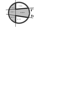
Figure 1: Example: patterns inside the grey region belong to one class, those in the white region to the other. The lines (labelled 1, 2 and 3) represent the hyperplanes found with the NetLines strategy. The arrows point into the correspondent positive half-spaces. The IRs of each domain are indicated (the first component, $\sigma_{0}=1$, is omitted for clarity).

2.3 The Algorithm NetLines

Like most adaptive learning algorithms, NetLines combines a growth heuristics with a particular learning algorithm for training the individual units, which are simple perceptrons. In this section we present the growth heuristics first, followed by the description of Minimerror, our perceptron learning algorithm.

Let us first introduce the following useful remark: if a neuron has to learn a target $\tau$, and the learnt state turns out to be $\sigma$, then the product $\sigma\tau=1$ if the target has been correctly learnt, and $\sigma\tau=-1$ otherwise.

Given a maximal accepted number of hidden units, $H_{max}$, and a maximal number of tolerated training errors, $E_{max}$, the algorithm may be summarized as follows:

Algorithm NetLines

• initialize
  ${\bf h=0}$;
  set the targets $\tau_{h+1}^{\mu}=\tau^{\mu}$ for $\mu=1,\cdots,P$;

• repeat

  1. /* train the hidden units */
     ${\bf h=h+1}$; /* connect hidden unit $h$ to the inputs */
     learn the training set $\{\vec{\xi}^{\mu},\tau_{h}^{\mu}\}$, $\mu=1,\cdots,P$;
     after learning, $\sigma_{h}^{\mu}={\rm sign}(\vec{w}_{h}\cdot{\vec{\xi}}^{\mu})$, $\mu=1,\cdots,P$;
     if $h=1$ /* for the first hidden neuron */
     

     if $\sigma_{1}^{\mu}=\tau_{1}^{\mu}$ $\forall\mu$ then stop. /* the training set is LS */;

     else set $\tau_{h+1}^{\mu}=\sigma_{h}^{\mu}\tau^{\mu}$ for $\mu=1,\cdots,P$; go to 1;

     end if

  2. /* learn the mapping between the IRs and the outputs */
     connect the output neuron to the $h$ trained hidden units;
     learn the training set $\{\vec{\sigma}^{\mu}(h),\tau^{\mu}\}$; $\mu=1,\cdots,P$;
     after learning, $\zeta^{\mu}(h)={\rm sign}\left(\vec{W}(h)\cdot\vec{\sigma}^{\mu}\right)$, $\mu=1,\cdots,P$;
     set $\tau_{h+1}^{\mu}=\zeta^{\mu}\tau^{\mu}$ for $\mu=1,\cdots,P$;
     count the number of training errors $e=\sum_{\mu}(1-\tau_{h+1}^{\mu})/2$;

• until $(h=H_{max}$ or $e\leq E_{max})$;

The generated network has $H=h$ hidden units. In the Appendix we present a solution to the learning strategy with a bounded number of hidden units. In practice the algorithm ends up with much smaller networks than this upper bound, as will be shown in Section 5.

2.4 The perceptron learning algorithm

The final number of hidden neurons, which are simple perceptrons, depends on the performance of the learning algorithm used to train them. The best solution should minimize the number of errors; if the training set is LS it should endow the units with the lowest generalization error. Our incremental algorithm uses Minimerror [20] to train the hidden and output units. Minimerror is based on the minimization of a cost function $E$ that depends on the perceptron weights $\vec{w}$ through the stabilities of the training patterns. If the input vector is $\vec{\xi}^{\mu}$ and $\tau^{\mu}$ the corresponding target, then the stability $\gamma^{\mu}$ of pattern $\mu$ is a continuous and derivable function of the weights, given by:

$$\gamma^{\mu}=\tau^{\mu}\frac{\vec{w}\cdot\vec{\xi}^{\mu}}{\parallel\vec{w}\parallel}$$ (3)

where $\parallel\vec{w}\parallel=\sqrt{\vec{w}\cdot\vec{w}}$. The stability is independent of the norm of the weights $\parallel\vec{w}\parallel$. It measures the distance of the pattern to the separating hyperplane, which is normal to $\vec{w}$; it is positive if the pattern is well classified, negative otherwise. The cost function $E$ is:

$$E=\frac{1}{2}\sum_{\mu=1}^{P}\left[1-\tanh\frac{\gamma^{\mu}}{2T}\right]$$ (4)

The contribution to $E$ of patterns with large negative stabilities is $\simeq 1$, i.e. they are counted as errors, whereas the contribution of patterns with large positive stabilities is vanishingly small. Patterns at both sides of the hyperplane within a window of width $\approx 4T$ contribute to the cost function even if they have positive stability.

The properties of the global minimum of (4) have been studied theoretically with methods of statistical mechanics [21]. It was shown that in the limit $T\rightarrow 0$, the minimum of $E$ corresponds to the weights that minimize the number of training errors. If the training set is LS, these weights are not unique [24]. In that case, there is an optimal learning temperature such that the weights minimizing $E$ at that temperature endow the perceptron with a generalization error numerically indistinguishable from the optimal (bayesian) value.

The algorithm Minimerror [20, 33] implements a minimization of $E$ restricted to a sub-space of normalized weights, through a gradient descent combined with a slow decrease of the temperature $T$, which is equivalent to a deterministic annealing. It has been shown that the convergence is faster if patterns with negative stabilities are considered at a temperature $T_{-}$ larger than those with positive stabilities, $T_{+}$, with a constant ratio $\theta=T_{-}/T_{+}$. The weights and the temperatures are iteratively updated through:

$$\delta\vec{w}(t) = \epsilon\left[\sum_{\mu/\gamma^{\mu}\leq 0}\frac{\tau^{\mu}\vec{\xi}^{\mu}}{\cosh^{2}(\gamma^{\mu}/2T_{-})}+\sum_{\mu/\gamma^{\mu}>0}\frac{\tau^{\mu}\vec{\xi}^{\mu}}{\cosh^{2}(\gamma^{\mu}/2T_{+})}\right]$$ (5)

$$T_{+}^{-1}(t+1) = T_{+}^{-1}(t)+\delta T^{-1};\,\,T_{-}=\theta T_{+};$$ (6)

$$\vec{w}(t+1) = \sqrt{N+1}\frac{\vec{w}(t)+\delta\vec{w}(t)}{\parallel\vec{w}(t)+\delta\vec{w}(t)\parallel}$$ (7)

Notice from (5) that only the incorrectly learned patterns at distances shorter than $\approx 2T_{-}$ from the hyperplane, and those correctly learned lying closer than $\approx 2T_{+}$, contribute effectively to learning. The contribution of patterns outside this region are vanishingly small. By decreasing the temperature, the algorithm selects to learn patterns increasingly localized in the neighborhood of the hyperplane, allowing for a highly precise determination of the parameters defining the hyperplane, which are the neuron’s weights. Normalization (7) restricts the search to the sub-space with $\parallel\vec{w}\parallel=\sqrt{N+1}$.

The only adjustable parameters of the algorithm are the temperature ratio $\theta=T_{-}/T_{+}$, the learning rate $\epsilon$ and the annealing rate $\delta T^{-1}$. In principle they should be adapted to each specific problem. However, thanks to our normalizing the weights to $\sqrt{N+1}$ and to data standardization (see next section), all the problems are brought to the same scale, simplifying the choice of the parameters.

2.5 Data standardization

Instead of determining the best parameters for each new problem, we standardize the input patterns of the training set through a linear transformation, applied to each component:

$$\tilde{\xi}_{i}^{\mu}=\frac{\xi_{i}^{\mu}-\langle\xi_{i}\rangle}{\Delta_{i}};\;1\leq i\leq N$$ (8)

The mean $\langle\xi_{i}\rangle$ and the variance $\triangle_{i}^{2}$, defined as usual:

$$\langle\xi_{i}\rangle = \frac{1}{P}\sum_{\mu=1}^{P}\xi_{i}^{\mu}$$ (9)

$${\Delta_{i}}^{2} = \frac{1}{P}\sum_{\mu=1}^{P}{({\xi_{i}^{\mu}-\langle\xi_{i}\rangle})}^{2}=\frac{1}{P}\sum_{\mu=1}^{P}(\xi_{i}^{\mu})^{2}-(\langle\xi_{i}\rangle)^{2}$$ (10)

need only a single pass of the $P$ training patterns to be determined. After learning, the inverse transformation is applied to the weights,

$$\tilde{w}_{0} = \sqrt{N+1}\frac{w_{0}-\sum\limits_{i=1}^{N}w_{i}\langle\xi_{i}\rangle/\Delta_{i}}{\sqrt{\left[w_{0}-\sum_{j=1}^{N}w_{j}\langle\xi_{j}\rangle/\Delta_{j}\right]^{2}+\sum_{j=1}^{N}(w_{j}/\Delta_{j})^{2}}}$$ (11)

$$\tilde{w}_{i} = \sqrt{N+1}\frac{w_{i}/\Delta_{i}}{\sqrt{\left[w_{0}-\sum_{j=1}^{N}w_{j}\langle\xi_{j}\rangle/\Delta_{j}\right]^{2}+\sum_{j=1}^{N}(w_{j}/\Delta_{j})^{2}}}$$ (12)

so that the normalization (8) is completely transparent to the user: with the transformed weights (11) and (12) the neural classifier is applied to the data in the original user’s units, which do not need to be renormalized.

As a consequence of the weights scaling (7) and the inputs standardization (8), all the problems are automatically rescaled. This allows us to use always the same values of Minimerror’s parameters, namely, the ”standard” values $\epsilon=0.02$, $\delta T^{-1}=10^{-3}$ and $\theta=6$. They were used throughout this paper, the reported results being highly insensitive to slight variations of them. However, in some extremely difficult cases, like learning the parity in dimensions $N>10$ and finding the separation of the sonar signals (see section 5), larger values of $\theta$ were needed.

2.6 Interpretation

It has been shown [22] that the contribution of each pattern to the cost function of Minimerror, $\left[1-\tanh(\gamma^{\mu}/2T)\right]/2$, may be interpreted as the probability of misclassification at the temperature $T$ at which the minimum of the cost function has been determined. By analogy, the neuron’s prediction on a new input $\vec{\xi}$ may be given a confidence measure by replacing the (unknown) pattern stability by its absolute value $\parallel\gamma\parallel=\parallel\vec{w}\cdot\vec{\xi}\parallel/\parallel\vec{w}\parallel$, which is its distance to the hyperplane. This interpretation of the sigmoidal function $\tanh(\parallel\gamma\parallel/2T)$ as the confidence on the neuron’s output is similar to the one proposed earlier [18] within an approach based on information theory.

The generalization of these ideas to multilayered networks is not straightforward. An estimate of the confidence on the classification by the output neuron should include the magnitude of the weighted sums of the hidden neurons, as they measure the distances of the input pattern to the domain boundaries. However, short distances to the separating hyperplanes are not always correlated to low confidence on the network’s output. For an example, we refer again to figure 1. Consider a pattern lying close to hyperplane 1. A small weighted sum on neuron 1 may cast doubt on the classification if the pattern’s IR is (-++), but not if it is (-+-), as a change of the sign of the weighted sum in the latter case will map the pattern to the IR (++-) which, being another IR of the same class, will be given the same output by the network. It is worth noting that the same difficulty is met by the interpretation of the outputs of multilayered perceptrons, trained with Backpropagation, as posterior probabilities. We do not go on further into this problem, which is beyond the scope of this paper.

3 Comparison with other strategies

There are few learning algorithms for neural networks composed of binary units. To our knowledge, all of them are incremental. In this section we give a short overview of some of them, in order to put forward the main differences with NetLines. We discuss the growth heuristics first, and the individual units training algorithms afterwards.

The Tiling algorithm [29] introduces hidden layers, one after the other. The first neuron of each layer is trained to learn an IR that helps to decrease the number of training errors; supplementary hidden units are then appended to the layer until the IRs of all the patterns in the training set are faithful. This procedure may generate very large networks. The Upstart algorithm [11] introduces successive couples of daughter hidden units between the input layer and the previously included hidden units, which become their parents. The daughters are trained to correct the parents classification errors, one daughter for each class. The obtained network has a tree-like architecture. There are two different algorithms implementing the Tilinglike Learning in the Parity Machine [2], Offset [28] and MonoPlane [38]. In both algorithms, each appended unit is trained to correct the errors of the previously included unit in the same hidden layer, a procedure that has been shown to generate a parity machine: the class of the input patterns is the parity of the learnt IRs. Unlike Offset, which implements the parity through a second hidden layer, that needs to be pruned, MonoPlane goes on adding hidden units (if necessary) in the same hidden layer until the number of training errors at the output vanishes. Convergence proofs for binary input patterns have been produced for all these algorithms. In the case of real-valued input patterns, a solution to the parity machine with a bounded number of hidden units also exists [19].

The rationale behind the construction of the parity machine is that it is not worth training the output unit before all the training errors of the hidden units have been corrected. However, Marchand et al. [27] pointed out that it is not necessary to correct all the errors of the successively trained hidden units: it is sufficient that the IRs be faithful and LS. If the output unit is trained immediately after each appended hidden unit, the network may discover that the IRs are already faithful and stop adding units. This may be seen on the example of figure 1. None of the parity machine implementations would find the solution represented on the figure, as each of the 3 perceptrons unlearns systematically part of the patterns learnt by the preceding one.

To our knowledge, Sequential Learning [27] is the only incremental learning algorithm that might find a solution equivalent (although not the same) to the one of figure 1. In this algorithm, the first unit is trained to separate the training set keeping one ”pure” half-space, i.e. a half space only containing patterns of one class. Wrongly classified patterns, if any, must all lie in the other half-space. Each appended neuron is trained to separate wrongly classified patterns with this constraint, i.e. keeping always one ”pure”, error-free, half-space. Thus, neurons must be appended in a precise order, making the algorithm difficult to implement in practice. For example, Sequential Learning applied to the problem of figure 1 needs to impose that the first unit finds the weights $\vec{w}_{3}$, as this is the only solution satisfying the purity restriction.

Other proposed incremental learning algorithms strive to solve the problem with different architectures, and/or with real valued units. For example, in the algorithm Cascade Correlation [9], each appended unit is selected among a pool of several real-valued neurons, trained to learn the correlation between the targets and the training errors. The unit is then connected to the input units and to all the other hidden neurons already included in the network.

Another approach to learning classification tasks is through the construction of decision trees [5], which partition hierarchically the input space through successive dichotomies. The neural networks implementations generate tree-like architectures. Each neuron of the tree introduces a dichotomy of the input space which is treated separately by the children nodes, which eventually produce new splits. Besides the weights, the resulting networks need to store the decision path. The proposed heuristics [36, 10, 26] differ in the algorithm used to train each node, and/or in the stopping criterium. In particular, Neural-Trees [36] may be regarded as a generalization of CART [5] in which the hyperplanes are not constrained to be perpendicular to the coordinate axis. The heuristics of the Modified Neural Tree Network [10], similar to Neural-Trees, includes a criterium of early stopping based on a confidence measure of the partition. As NetLines considers the whole input space to train each hidden unit, it generates domain boundaries which may greatly differ from the splits produced by trees. We are not aware of any systematic study nor theoretical comparison of both approaches.

Other algorithms, like RCE [34], GAL [1], Glocal [7] and Growing cells [14] propose to cover or mask the input space with hyperspheres of adaptive size containing patterns of the same class. These approaches generally end up with a very large number of units. Covering Regions by the LP Method [30] is a trial and error procedure devised to select the most efficient masks among hyperplanes, hyperspheres or hyperellipsoids. The mask’s parameters are determined through linear programming.

Many incremental strategies use the Pocket algorithm [15] to train the appended units. Its main drawback is that it has no natural stopping condition, which is left to the user’s patience. The proposed alternative algorithms [12, 3] are not guaranteed to find the best solution to the problem of learning. The algorithm used by the Modified Neural Tree Network (MNTN) [10] and the ITRULE [18] minimize cost functions similar to (4), but using different misclassification measures at the place of our stability (3). The essential difference with Minimerror is that none of these algorithms are able to control which patterns contribute to learning, like Minimerror does with the temperature.

4 Generalization to Multi-class Problems

The usual way to cope with problems having more than two classes, is to generate as many networks as classes. Each network is trained to separate patterns of one class from all the others, and a winner-takes-all (WTA) strategy based on the value of output’s weighted sum in equation (2) is used to decide the class if more than one network recognizes the input pattern. As we use normalized weights, in our case the output’s weighted sum is merely the distance of the IR to the separating hyperplane. All the patterns mapped to the same IR are given the same output’s weighted sum, independently of the relative position of the pattern in input space. As already discussed in section 2.6, a strong weighted sum on the output neuron is not inconsistent with small weighted sums on the hidden neurons. Therefore, a naive WTA decision may not give good results, as is shown in the example of section 5.3.1.

We now describe an implementation for the multi-class problem that results in a tree-like architecture of networks. It is more involved that the naive WTA, and may be applied to any binary classifier. Suppose that we have a problem with $C$ classes. We must choose in which order the classes will be learnt, say $(c_{1},c_{2},\cdots,c_{C})$. This order constitutes a particular learning sequence. Given a particular learning sequence, a first network is trained to separate class $c_{1}$, which is given output target $\tau_{1}=+1$, from the others (which are given targets $\tau_{1}=-1$). The opposite convention is equivalent, and could equally be used. After training, all the patterns of class $c_{1}$ are eliminated from the training set and we generate a second network trained to separate patterns of class $c_{2}$ from the remaining classes. The procedure, reiterated with training sets of decreasing size, generates $C-1$ hierarchically organized tree of networks (TON): the outputs are ordered sequences $\vec{\zeta}=(\zeta_{1},\zeta_{2},\cdots,\zeta_{C-1})$. The predicted class of a pattern is $c_{i}$, where $i$ is the first network in the sequence having an output $+1$ ($\zeta_{i}=+1$ and $\zeta_{j}=-1$ for $j<i$), the outputs of the networks with $j>i$ being irrelevant.

The performance of the TON may depend on the chosen learning sequence. Therefore, it is convenient that an odd number of TONs, trained with different learning sequences, compete through a vote. We verified empirically, as is shown in section 5.3, that this vote improves the results obtained with each of the individual TONs participating to the vote. Notice that our procedure is different from bagging [4], as all the networks of the TON are trained with the same training set, without the need of any resampling procedure.

5 Applications

Although convergence proofs of learning algorithms are satisfactory on theoretical grounds, they are not a guarantee of good generalization. In fact, they only demonstrate that correct learning is possible, but do not address the problem of generalization. This last issue still remains quite empirical [40, 17, 13], and the generalization performance of learning algorithms is usually tested on well known benchmarks [32].

We first tested the algorithm on learning the parity function of $N$ bits for $2\leq N\leq 11$. It is well known that the smallest network with the architecture considered here needs $H=N$ hidden neurons. The optimal architecture was found in all the cases. Although this is quite an unusual performance, the parity is not a representative problem: learning is exhaustive and generalization cannot be tested. Another test, the classification of sonar signals [23], revealed the quality of Minimerror, as it solved the problem without hidden units. In fact, we found that not only the training set of this benchmark is linearly separable, a result already reported [25, 35], but that the complete data base, i.e. the training and the test sets together, are also linearly separable.

We present next our results, generalization error $\epsilon_{g}$ and number of weights, on several benchmarks corresponding to different kinds of problems: binary classification of binary input patterns, binary classification of real-valued input patterns, and multi-class problems. These benchmarks were chosen because they served already as a test to many other algorithms, providing unbiased results to compare with. The generalization error $\epsilon_{g}$ of NetLines was estimated as usual, through the fraction of misclassified patterns on a test set of data.

The results are reported as a function of the training sets sizes $P$ whenever these sizes are not specified by the benchmark. Besides the generalization error $\epsilon_{g}$, averaged over a (specified) number of classifiers trained with randomly selected training sets, we present also the number of weights of the corresponding networks. The latter is a measure of the classifier’s complexity, as it corresponds to the number of its parameters.

Training times are usually cited among the characteristics of the training algorithms. Only the numbers of epochs used by Backpropagation on two of the studied benchmarks have been published; we restrict the comparison to these cases. As NetLines only updates $N$ weights per epoch, whereas Backpropagation updates all the network’s weights, we compare the total number of weights updates. They are of the same order of magnitude for both algorithms. However, these comparisons should be taken with caution. NetLines is a deterministic algorithm: it learns the architecture and the weights through one single run, whereas with Backpropagation several architectures must be previously investigated, and this time is not included in the training time.

The following notation is used: $D$ is the total number of available patterns, $P$ the number of training patterns, $G$ the number of test patterns.

5.1 Binary inputs

The case of binary input patterns has the property, not shared by real-valued inputs, that every pattern may be separated from the others by a single hyperplane. This solution, usually called grand-mother, needs as many hidden units as patterns in the training set. In fact, the convergence proofs for incremental algorithms in the case of binary input patterns are based on this property.

5.1.1 Monk’s problem

This benchmark, thoroughly studied with many different learning algorithms [39], contains three distinct problems. Each one has an underlying logical proposition that depends on six discrete variables, coded with $N=17$ binary numbers. The total number of possible input patterns is $D=432$, and the targets correspond to the truth table of the corresponding proposition. Both NetLines and MonoPlane found the underlying logical proposition of the first two problems, i.e. they generalized correctly giving $\epsilon_{g}=0$. In fact, these are easy problems: all the neural network-based algorithms, and some non-neural learning algorithms were reported to correctly generalize them. In the third Monk’s problem, 6 patterns among the $P_{3}=122$ examples are given wrong targets. The generalization error is calculated over the complete set of $D=432$ patterns, i.e. including the training patterns, but in the test set all the patterns are given the correct targets. Thus, any training method that learns correctly the training set will make at least $1.4\%$ of generalization errors. Four algorithms specially adapted to noisy problems were reported to reach $\epsilon_{g}=0$. However, none of them generalizes correctly the two other (noiseless) Monk’s problems. Besides them, the best performance, $\epsilon_{g}=0.0277$ which corresponds to 12 misclassified patterns, is only reached by neural networks methods: Backpropagation, Backpropagation with Weight Decay, Cascade-Correlation and NetLines. The number of hidden units generated with NetLines ($58$ weights) is intermediate between Backpropagation with weight decay ($39$), and Cascade-Correlation ($75$) or Backpropagation ($77$). MonoPlane reached a slightly worse performance ($\epsilon_{g}=0.0416$, i.e. 18 misclassified patterns) with the same number of weights as NetLines, showing that the parity machine encoding may not be optimal.

5.1.2 Two or more clumps

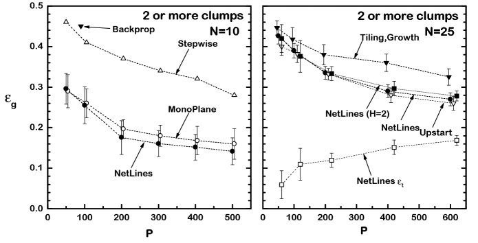
Figure 2: Two or more clumps for two ring sizes, $N=10$ and $N=25$. Generalization error $\epsilon_{g}$ vs. size of the training set $P$, for different algorithms. $N=10$: Backpropagation [37], Stepwise [26]. $N=25$: Tiling [29], Upstart [11]. Results with the Growth Algorithm [31] are indistinguishable from those of Tiling at the scale of the figure. Points without error bars correspond to best results. Results of MonoPlane and NetLines are averages over 25 tests.

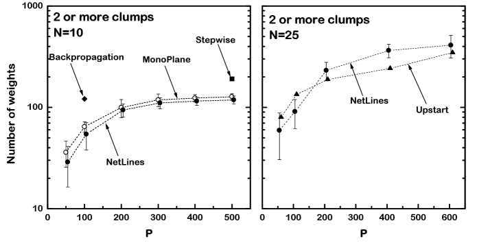
Figure 3: Two or more clumps. Number of weights (logarithmic scale) vs. size of the training set $P$, for $N=10$ and $N=25$. Results of MonoPlane and NetLines are averages over 25 tests. The references are the same as in figure 2.

In this problem [6] the network has to discriminate if the number of clumps in a ring of $N$ bits is strictly smaller than 2 or not. One clump is a sequence of identical bits bounded by bits of the other kind. The patterns are generated through a MonteCarlo method in which the mean number of clumps is controlled by a parameter $k$ [29]. We generated training sets of $P$ patterns with $k=3$, corresponding to a mean number of clumps of $\approx 1.5$, for rings of $N=10$ and $N=25$ bits. The generalization error corresponding to several learning algorithms, estimated with independently generated testing sets of the same sizes as the training sets, i.e. $G=P$, are displayed on figures 2 as a function of $P$. Points with error bars correspond to averages over 25 independent training sets. Points without error bars correspond to best results. NetLines, MonoPlane and Upstart for $N=25$ have nearly the same performances when trained to reach error-free learning.

We tested the effect of early stopping by imposing to NetLines a maximal number of two hidden units ($H=2$). The residual training error $\epsilon_{t}$ is plotted on the same figure, as a function of $P$. It may be seen that early-stopping does not help to decrease $\epsilon_{g}$. Overfitting, that arises when NetLines is applied until error-free training is reached, does not degrade the network’s generalization performance. This behavior is very different from the one of networks trained with Backpropagation. The latter reduces classification learning to a regression problem, in which the generalization error can be decomposed in two competing terms: bias and variance. With Backpropagation, early stopping helps to decrease overfitting because some hidden neurons do not reach large enough weights to work in the non-linear part of the sigmoidal transfer functions. It is well known that all the neurons working in the linear part may be replaced by a single linear unit. Thus, with early-stopping, the network is equivalent to a smaller one, i.e. having less parameters, with all the units working in the non-linear regime. Our results are consistent with recent theories [13] showing that, contrary to regression, the bias and variance components of the generalization error in classification combine in a highly non-linear way.

The number of weights used by the different algorithms is plotted on a logarithmic scale as a function of $P$ on figures 3. It turns out that the strategy of NetLines is slightly better than that of MonoPlane, with respect to both generalization performance and network size.

5.2 Real valued inputs

We tested NetLines on two problems which have real valued inputs (we include graded-valued inputs here).

5.2.1 Wisconsin Breast Cancer Data Base

The input patterns of this benchmark [42] have $N=9$ attributes characterizing samples of breast cytology, classified as benign or malignant. We excluded from the original data base 16 patterns that have the attribute $\xi_{6}$ ("bare nuclei") missing. Among the remaining $D=683$ patterns, the two classes are unevenly represented, 65.5% of the examples being benign. We studied the generalization performance of networks trained with sets of several sizes $P$. The $P$ patterns for each learning test were selected at random. On figure  4a, the generalization error at classifying the remaining $G\equiv D-P$ patterns is displayed as a function of the corresponding number of weights in a logarithmic scale. For comparison, we included in the same figure results of a single perceptron trained with $P=75$ patterns using Minimerror. The results, averaged values over 50 independent tests for each $P$, show that both NetLines and MonoPlane have lower $\epsilon_{g}$ and less number of parameters than other algorithms on this benchmark.

The total number of weights updates needed by NetLines, including the weights of the dropped output units, is $7\cdot 10^{4}$; Backpropagation needed $\approx 10^{4}$ [32].

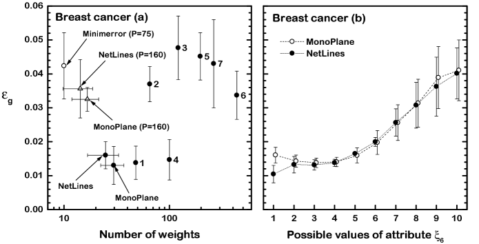
Figure 4: Breast cancer classification. (a) Generalization error $\epsilon_{g}$ vs. number of weights (logarithmic scale), for $P=525$. 1, 2, 3: Rprop with no shortcuts [32]; 4, 5, 6: Rprop with shortcuts [32]; 7: Cascade Correlation [7]. For comparison, results with smaller training sets, $P=75$ (single perceptron) and $P=160$, patterns are displayed. Results of MonoPlane and NetLines are averages over 50 tests. (b) Classification errors vs. possible values of the missing attribute ”bare nuclei” for the 16 incomplete patterns, averaged over 50 independently trained networks.

The trained network may be used to classify the patterns with missing attributes. The number of misclassified patterns among the 16 cases for which attribute $\xi_{6}$ is missing, is plotted as a function of the possible values of $\xi_{6}$ on figure  4b. For large values of $\xi_{6}$ there are discrepancies between the medical and the network’s diagnosis on half the cases. This is an example of the kind of information that may be obtained in practical applications.

5.2.2 Diabetes diagnosis

This benchmark [32] contains $D=768$ patterns described by $N=8$ real-valued attributes, corresponding to $\approx 35\%$ of Pima women suffering from diabetes, $65\%$ being healthy. Training sets of $P=576$ patterns were selected at random, and generalization was tested on the remaining $G=192$ patterns. The comparison with published results obtained with other algorithms tested under the same conditions, presented on figure  5, shows that NetLines reaches the best performances published so far on this benchmark, needing much less parameters. Training times of NetLines are of $\approx 10^{5}$ updates. The numbers of updates needed by Rprop [32] range between $4\cdot 10^{3}$ and $5\cdot 10^{5}$, depending on the network’s architecture.

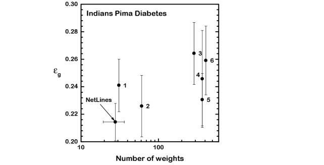
Figure 5: Diabetes diagnosis: Generalization error $\epsilon_{g}$ vs. number of weights. Results of NetLines are averages over $50$ tests. 1,2,3: Rprop no shortcuts, 4,5,6: Rprop with shortcuts [32]

5.3 Multi-class problems

We applied our learning algorithm to two different problems, both of three classes. We compare the results obtained with a winner-takes-all (WTA) classification based on the results of three networks, each one independently trained to separate one class from the two others, to the results of the TON architectures described in section 4. As the number of classes is low, we determined the three TONs, corresponding to the three possible learning sequences. The vote of the three TONs improves the performances, as expected.

5.3.1 Breiman’s Waveform Recognition Problem

This problem was introduced as a test for the algorithm CART [5]. The input patterns are defined by $N=21$ real-valued amplitudes $x(t)$ observed at regularly spaced intervals $t=1,2,\cdots,N$. Each pattern is a noisy convex linear combination of two among three elementary waves (triangular waves centered on three different values of $t$). There are three possible combinations, and the pattern’s class identifies from which combination it is issued.

We trained the networks with the same $11$ training sets of $P=300$ examples, and generalization was tested on the same independent test set of $G=5000$, as in [16]. Our results are displayed on figure 6, where only results of algorithms reaching $\epsilon_{g}<0.25$ in [16] are included. Although it is known that, due to the noise, the classification error has a lower bound of $\approx 14\%$ [5], the results of NetLines and MonoPlane presented here correspond to error-free training. The networks generated by NetLines have between 3 and 6 hidden neurons, depending on the training sets. The results obtained with a single perceptron trained with Minimerror and with the Perceptron learning algorithm, which may be considered as the extreme case of early stopping, are hardly improved by the more complex networks. Here again the overfitting produced by error-free learning with NetLines does not deteriorate the generalization performance. The TONs vote reduces the variance, but does not decrease the average $\epsilon_{g}$.

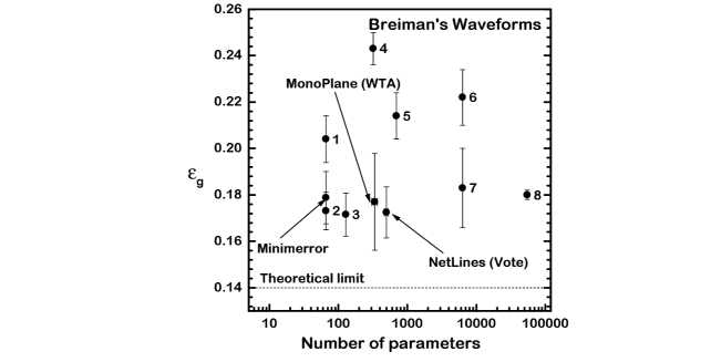
Figure 6: Breiman waveforms: Generalization error $\epsilon_{g}$ averaged over 11 tests vs. number of parameters. Error bars on the number of weights generated by NetLines and MonoPlane are not visible at the scale of the figure. 1: Linear disc., 2: Perceptron, 3: Backpropagation, 4: Genetic algorithm, 5: Quadratic disc., 6: Parzen’s kernel. 7: K-NN, 8: Constraint [16]

5.3.2 Fisher’s Iris plants database

In this classical three-class problem, one has to determine the class of Iris plants, based on the values of $N=4$ real-valued attributes. The database of $D=150$ patterns, contains $50$ examples of each class. Networks were trained with $P=149$ patterns, and the generalization error is the mean value of all the $150$ leave-one-out possible tests. Results of $\epsilon_{g}$ are displayed as a function of the number of weights on figure 7. Error bars are available only for our own results. In this hard problem, the vote of the three possible TONs trained with the three possible class sequences (see section 4) improves the generalization performance.

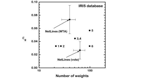
Figure 7: Iris database: Generalization error $\epsilon_{g}$ vs. number of parameters. 1: Offset, 2: Backpropagation [28]; 4,5: Backpropagation [41]; 3,6: GOT [41].

6 Conclusion

We presented an incremental learning algorithm for classification, that we call NetLines for Neural Encoder Through Linear Separation. It generates small feedforward neural networks with a single hidden layer of binary units connected to a binary output neuron. NetLines allows for an automatic adaptation of the neural network to the complexity of the particular task. This is achieved by coupling an error correcting strategy for the successive addition of hidden neurons with Minimerror, a very efficient perceptron training algorithm. Learning is fast, not only because it reduces the problem to that of training single perceptrons, but mainly because there is no longer need of the usual preliminary tests necessary to determine the correct architecture for the particular application. Theorems valid for binary as well as for real-valued inputs guarantee the existence of a solution with a bounded number of hidden neurons obeying the growth strategy.

The networks are composed of binary hidden units whose states constitute a faithful encoding of the input patterns. They implement a mapping from the input space to a discrete $H$-dimensional hidden space, $H$ being the number of hidden neurons. Thus, each pattern is labelled with a binary word of $H$ bits. This encoding may be seen as a compression of the pattern’s information. The hidden neurons define linear boundaries, or portions of boundaries, between classes in input space. The network’s output may be given a probabilistic interpretation based on the distance of the patterns to these boundaries.

Tests on several benchmarks showed that the networks generated by our incremental strategy are small, in spite of the fact that the hidden neurons are appended until error-free learning is reached. Even in those cases where the networks obtained with NetLines are larger than those used by other algorithms, its generalization error remains among the smallest values reported. In noisy or difficult problems it may be useful to stop the network’s growth before the condition of zero training errors is reached. This decreases overfitting, as smaller networks (with less parameters) are thus generated. However, the prediction quality (measured by the generalization error) of the classifiers generated with NetLines are not improved by early-stopping.

The results presented in this paper were obtained without cross-validation, nor any data manipulation like boosting, bagging or arcing [4, 8]. Those costly procedures combine results of very large numbers of classifiers, with the aim of improving the generalization performance through the reduction of the variance. As NetLines is a stable classifier, presenting small variance, we do not expect that such techniques would significantly improve our results.

Appendix

In this Appendix we exhibit a particular solution to the learning strategy of NetLines. This solution is built in such a way that the cardinal of a convex subset of well learnt patterns, $L_{h}$, grows monotonically upon the addition of hidden units. As this cardinal cannot be larger that the total number of training patterns, the algorithm must stop with a finite number of hidden units.

Suppose that $h$ hidden units have already been included and that the output neuron still makes classification errors on patterns of the training set, called training errors. Among these wrongly learned patterns, be $\nu$ the one closest to the hyperplane normal to $\vec{w}_{h}$, called hyperplane-$h$ hereafter. We define $L_{h}$ as the subset of (correctly learnt) patterns laying closer to the hyperplane-$h$ than $\vec{\xi}^{\nu}$. Patterns in $L_{h}$ have $0<\gamma_{h}<|\gamma_{h}^{\nu}|$. The subset $L_{h}$ and at least pattern $\nu$ are well learnt if the next hidden unit, $h+1$, has weights:

$$\vec{w}_{h+1}=\tau_{h}^{\nu}\vec{w}_{h}-(1-\epsilon_{h})\tau_{h}^{\nu}(\vec{w}_{h}\cdot\vec{\xi}^{\nu})\hat{e}_{0}$$ (13)

where $\hat{e}_{0}\equiv(1,0,\cdots,0)$. The conditions that both $L_{h}$ and pattern $\nu$ have positive stabilities (i.e. be correctly learned) impose that

$$0<\epsilon_{h}<\min_{\mu\in L_{h}}\frac{|\gamma_{h}^{\nu}|-\gamma_{h}^{\mu}}{|\gamma_{h}^{\nu}|}$$ (14)

The following weights between the hidden units and the output will give the correct output to pattern $\nu$ and to the patterns of $L_{h}$:

$$W_{0}(h+1) = W_{0}(h)+\tau^{\nu}$$ (15)

$$W_{i}(h+1) = W_{i}(h)\;for\;1\leq i\leq h$$ (16)

$$W_{h+1}(h+1) = -\tau^{\nu}$$ (17)

Thus, $card(L_{h+1})\geq card(L_{h})+1$. As the number of patterns in $L_{h}$ increases monotonically with $h$, convergence is guaranteed with less than $P$ hidden units.

References

- [1] Alpaydin, E.A.I. 1990. Neural models of supervised and unsupervised learning. Ph.D. thesis, EPFL 863, Lausanne, Suisse.
- [2] Biehl, M., & Opper, M. 1991. Tilinglike learning in the parity machine. Physical review a, 44, 6888.
- [3] Bottou, L., & Vapnik, V. 1992. Local learning algorithms. Neural computation, 4(6), 888–900.
- [4] Breiman, L. September, 1994. Bagging predictors. Tech. rept. 421. Department of Statistics. University of California at Berkeley.
- [5] Breiman, L., Friedman, J. H., Olshen, R. A., & Stone, C. J. 1984. Classification and regression trees. Monterey, CA: Wadsworth and Brooks/Cole.
- [6] Denker, J., Schwartz, D., Wittner, B., Solla, S., Howard, R., Jackel, L., & Hopfield, J. 1987. Large automatic learning, rule extraction, and generalization. Complex systems, 1, 877–922.
- [7] Depenau, J. 1995. Automated design of neural network architecture for classification. Ph.D. thesis, EF-448, DAIMI, Computer Science Department, Aarhus University.
- [8] Drucker, Harris, Schapire, Robert, & Simard, Patrice. 1993. Improving performance in neural networks using a boosting algorithm. Pages 42–49 of: Hanson, Stephen José, Cowan, Jack D., & Giles, C. Lee (eds), Advances in neural information processing systems, vol. 5. Morgan Kaufmann, San Mateo, CA.
- [9] Fahlman, S.E., & Lebiere, C. 1990. The cascade-correlation learning architecture. Pages 524–532 of: Touretzky, D.S. (ed), Advances in neural information processing systems, vol. 2. San Mateo: Morgan Kaufmann, for (Denver 1989).
- [10] Farrell, Kevin R., & Mammone, Richard J. 1994. Speaker recognition using neural tree networks. Pages 1035–1042 of: Cowan, Jack D., Tesauro, Gerald, & Alspector, Joshua (eds), Advances in neural information processing systems, vol. 6. Morgan Kaufmann Publishers, Inc.
- [11] Frean, M. 1990. The upstart algorithm: A method for constructing and training feedforward neural networks. Neural computation, 2(2), 198–209.
- [12] Frean, M. 1992. A “thermal” perceptron learning rule. Neural computation, 4(6), 946–957.
- [13] Friedman, J.H. 1996. On bias, variance, 0/1 - loss, and the curse-of-dimensionality. Tech. rept. Department of Statistics. Stanford University.
- [14] Fritzke, Bernd. 1994. Supervised learning with growing cell structures. Pages 255–262 of: Cowan, Jack D., Tesauro, Gerald, & Alspector, Joshua (eds), Advances in neural information processing systems, vol. 6. Morgan Kaufmann Publishers, Inc.
- [15] Gallant, Stephen I. 1986. Optimal linear discriminants. Pages 849–852 of: Proc. 8th. conf. pattern recognition, oct. 28-31, paris, vol. 4.
- [16] Gascuel, O. 1995. Symenu. collective paper (gascuel o. coordinator). Tech. rept. 5 mes Journ es Nationales du PRC-IA Teknea, (Nancy).
- [17] Geman, S., Bienenstock, E., & Doursat, R. 1992. Neural networks and the bias/variance dilemma. Neural computation, 4(1), 1–58.
- [18] Goodman, R. M., Smyth, P., Higgins, C. M., & Miller, J. W. 1992. Rule-based neural networks for classification and probability estimation. Neural computation, 4(6), 781–804.
- [19] Gordon, M. 1996. A convergence theorem for incremental learning with real-valued inputs. Pages 381–386 of: Ieee international conference on neural networks.
- [20] Gordon, M.B., & Berchier, D. 1993. Minimerror: A perceptron learning rule that finds the optimal weights. Pages 105–110 of: Verleysen, Michel (ed), European symposium on artificial neural networks. Brussels: D facto.
- [21] Gordon, M.B., & Grempel, D. 1995. Optimal learning with a temperature dependent algorithm. Europhysics letters, 29(3), 257–262.
- [22] Gordon, M.B., Peretto, P., & Berchier, D. 1993. Learning algorithms for perceptrons from statistical physics. Journal of physics i france, 3, 377–387.
- [23] Gorman, R.P., & Sejnowski, T.J. 1988. Analysis of hidden units in a layered network trained to classify sonar targets. Neural networks, 1, 75–89.
- [24] Gyorgyi, G., & Tishby, N. 1990. Statistical theory of learning a rule. In: Theumann, W.K., & Koeberle, R. (eds), Neural networks and spin glasses. Singapore: World Scientific.
- [25] Hoehfeld, M., & Fahlman, S. 1991. Learning with limited numerical precision using the cascade correlation algorithm. Tech. rept. CMU-CS-91-130. Carnegie Mellon University.
- [26] Knerr, S., Personnaz, L., & Dreyfus, G. 1990. Single-layer learning revisited: a stepwise procedure for building and training a neural network. In: Neurocomputing, algorithms, architectures and applications. Elsevier.
- [27] Marchand, M., Golea, M., & Ruján, P. 1990. A convergence theorem for sequential learning in two-layer perceptrons. Europhysics letters, 11, 487–492.
- [28] Martinez, D., & Est ve, D. 1992. The offset algorithm: building and learning method for multilayer neural networks. Europhysics letters, 18, 95–100.
- [29] Mézard, M., & Nadal, J.-P. 1989. Learning in feedforward layered networks: the tiling algorithm. J. phys. a: Math. and gen., 22, 2191–203.
- [30] Mukhopadhyay, S., Roy, A., Kim, L. S., & Govil, S. 1993. A polynomial time algorithm for generating neural networks for pattern classification: Its stability properties and some test results. Neural computation, 5(2), 317–330.
- [31] Nadal, J.-P. 1989. Study of a growth algorithm for a feedforward neural network. Int. journ. of neur. syst., 1, 55–9.
- [32] Prechelt, L. 1994 (September). PROBEN1 - A set of benchmarks and benchmarking rules for neural network training algorithms. Tech. rept. 21/94. University of Karlsruhe, Faculty of Informatics.
- [33] Raffin, B., & Gordon, M.B. 1995. Learning and generalization with minimerror, a temperature dependent learning algorithm. Neural computation, 7(6), 1206–1224.
- [34] Reilly, D.E, Cooper, L.N., & Elbaum, C. 1982. A neural model for category learning. Biological cybernetics, 45, 35–41.
- [35] Roy, A., Kim, L., & Mukhopadhyay, S. 1993. A polynomial time algorithm for the construction and training of a class of multilayer perceptron. Neural networks, 6(1), 535–545.
- [36] Sirat, J. A., & Nadal, J.-P. 1990. Neural trees: a new tool for classification. Network, 1, 423–38.
- [37] Solla, S.A. 1989. Learning and generalization in layered neural networks: The contiguity problem. Pages 168–177 of: Personnaz, L., & Dreyfus, G. (eds), Neural networks from models to applications. Paris: I.D.S.E.T., for (Paris 1988).
- [38] Torres Moreno, J.-M., & Gordon, M. 1995. An evolutive architecture coupled with optimal perceptron learning for classification. Pages 365–370 of: Verleysen, Michel (ed), European symposium on artificial neural networks. Brussels: D facto.
- [39] Trhun, S.B., & co authors, 23. 1991. The monk’s problems. a performance comparison of different learning algorithms. Tech. rept. CMU-CS-91-197. Carnegie Mellon University.
- [40] Vapnik, V. 1992. Principles of risk minimization for learning theory. Pages 831–838 of: Moody, John E., Hanson, Steve J., & Lippmann, Richard P. (eds), Advances in neural information processing systems, vol. 4. Morgan Kaufmann Publishers, Inc.
- [41] Verma, Brijesh K., & Mulawka, Jan J. 1995. A new algorithm for feedforward neural networks. Pages 359–364 of: Verleysen, Michel (ed), European symposium on artificial neural networks. Brussels: D facto.
- [42] Wolberg, W.H., & Mangasarian, O.L. 1990. Multisurface method of pattern separation for medical diagnosis applied to breast cytology. Pages 9193–9196 of: Proceedings of the national academy of sciences, usa, vol. 87.