Optical properties of correlated materials –
Generalized Peierls approach and its application to VO₂

Abstract

The aim of the present paper is to present a versatile scheme for the computation of optical properties of solids, with particular emphasis on realistic many-body calculations for correlated materials. Geared at the use with localized basis sets, we extend the commonly known lattice “Peierls substitution” approach to the case of multi-atomic unit cells. We show in how far this generalization can be deployed as an approximation to the full Fermi velocity matrix elements that enter the continuum description of the response of a solid to incident light. We further devise an upfolding scheme to incorporate optical transitions, that involve high energy orbitals that had been downfolded in the underlying many-body calculation of the electronic structure. As an application of the scheme, we present results on a material of longstanding interest, vanadium dioxide, VO₂. Using dynamical mean-field data of both, the metallic and the insulating phase, we calculate the corresponding optical conductivities, elucidate optical transitions and find good agreement with experimental results.

I Introduction

Correlated matter is characterized by an enormous sensitivity with respect to changes of external parameters. It is the merit of this responsiveness that a remarkable richness of properties emerges in these systems. Correlation effects seem, for instance, to be a vital issue to outstanding phenomena such as high temperature superconductivity and colossal magnetoresistance. In the latter case, the possibility of tuning the fundamental behavior of a material by an external field will undoubtedly lead to yet improved data storage devices. A better understanding of the various effects of strong correlations is thus a highly desirable goal of condensed matter physics, both from the theoretical and the technological point of view.

On the experimental side, numerous techniques have been devised for and applied to the study of correlated materials of ever growing complexity. Optical spectroscopy, which is the subject of this paper, is, in a way, the most natural among them : Optical detectors are sampling the response to incident light, as do our eyes, albeit accessing frequencies, and thus phenomena, that are beyond our vision. The technique is particularly suited for tracking the evolution of the system under changes of, for instance, temperature or pressure. This is owing to a generally high precision, and the fact that, contrary to e.g. photoemission spectroscopy or x-ray experiments, results are obtained in absolute values. Especially, the existence of sum-rules allows for a quantitative assessment of transfers of spectral weight upon changes of the system properties. Therewith optical spectroscopy is particularly adapted to the study of correlated materials PhysRevB.73.165116 ; PCCO ; Qazilbash12142007 ; Baldassarre_v2o3 ; pnictide_optic .

On the theory side, while weakly correlated materials are well described within density functional theory (DFT)RevModPhys.71.1253 , e.g. in the local density approximation (LDA)kohn2 , and moderate correlation effects are captured by perturbative approaches, such as Hedin’s GW approximationhedin , it was the advent of dynamical mean-field theory (DMFT)(for reviews see e.g. bible ; vollkot ), and its realistic extension, LDA+DMFT (for reviews see held_psik ; biermann_ldadmft ), which allowed for the description and understanding of several metal-insulator transitions that are derived from the Mott-Hubbard or related mechanisms. Though our discussion of optical properties within realistic many-body approaches is quite general, and applicable to other techniques, we present results on VO₂ that are based on LDA+DMFT calculations.

The paper is organized as follows : After having now expanded on the potency of optical spectroscopy and the motivation for more theoretical efforts, we will in the remainder of Section I briefly review experimental and theoretical knowledge about vanadium dioxide. In Section II we develop our formalism for the optical conductivity within realistic calculations. Section III is devoted to a detailed discussion on Fermi velocities. This part contains our major innovations. Readers less interested in technical details are welcome to jump directly to Section IV, which presents our theoretical optics spectra for vanadium dioxide in both, the metallic and the insulating phase.

I.1 Vanadium dioxide – The material

I.1.1 Basic electronic structure

At its metal-insulator transition PhysRevLett.3.34 (T_c=340 K), VO₂ transforms from a metallic high temperature phase of rutile structure into an insulating monoclinic (M1) phase, in which the vanadium atoms pair up to form tilted dimers along the c-axis. This M1 phase was found to be non-magnetic pouget_review .

Over the decades several scenarios were evoked to explain the metal-insulator transition. This is not the emphasis of the current paper, and we shall only briefly summarize the basic electronic structure.

VO₂ has a vanadium 3d¹ configuration and the crystal field splits the 3d-manifold into t_2g and empty e${}_{g}^{\sigma}$ components. The former are further split into e${}_{g}^{\pi}$ and a_1g orbitals. In the rutile phase these orbitals overlap, accounting for the metallic character. In the M1 phase, the a_1g split into bonding/anti-bonding orbitals, due to the aforementioned vanadium dimerization.

The Goodenough scenario PhysRev.117.1442 ; goodenough_vo2 of the insulator advocates the structural effect of the unit-cell doubling due to the dimer formation as the main origin of the gap-formation, and thus attributes the insulating behavior to a Peierls transitionpeierls_book . Zylbersztejn and Mott PhysRevB.11.4383 on the other hand stressed the importance of local Coulomb interactions, and thought the transition to be of, what we call today, the Mott-Hubbard type. Experiments PhysRevLett.35.873 ; PhysRevB.10.1801 ; koethe:116402 ; haverkort:196404 ; eguchi_vo2 ; qazilbash:075107 were interpreted to support one or the other of the two scenarios. Important to note is that neither of the two phases are well-described within standard band-theory approaches. In the rutile phase these miss bandwidth-narrowing and satellite features, as seen e.g. in photoemission koethe:116402 , and the bad metal conductivity seen in transport measurements ladd_vo2 . In the M1 phase, the problem is even more fundamental, since band-theory fails to produce an insulating behaviorPhysRevLett.72.3389 ; eyert_vo2 ; korotin_vo2 . For reviews see e.g. imada ; me_phd . As we will detail later, the LDA+DMFT approach succeeds in describing the experimental findings of both, the metallic 0295-5075-69-6-984 ; liebsch:085109 ; biermann:026404 and the insulating biermann:026404 phase. As a matter of fact the current calculations of optical properties rely on our previous LDA+DMFT work biermann:026404 ; tomczak_vo2_proc ; me_vo2 which in particular extended on the interpretation of the nature of the insulating M1 phase. Compatibility with experimental results on the optical conductivity strengthens this picture. For the insulating phase, also GW type of calculations PhysRevB.60.15699 ; me_phd ; sakuma:075106 ; gatti:266402 as well as LDA+U based approaches korotin_vo2 ; Eckern_vo2 open the charge gap. Further, VO₂ has also been studied within cluster based methods, see e.g. tanaka_vo2 ; Mossanek2005189 ; mossanek:125112 .

I.1.2 Insights by optical measurements

Optical measurements on VO₂ were first performed by Barker et al.PhysRevLett.17.1286 , and Verleur et al.PhysRev.172.788 . By probing different orientations of single crystal samples, they evidenced an anisotropy in the optical response of the M1 insulator. More precisely, the conductivity depends on whether the electric field is parallel or perpendicular to the crystallographic rutile c-axis when going below the transition temperature. This is to be expected from the changes in the crystal-structure and the unit-cell doubling along the c-axis. This anisotropy was confirmed by ultraviolet reflectance measurements PhysRevB.41.4993 and x-ray experimentsPhysRevB.43.7263 ; koethe:116402 (see also PhysRevB.20.1546 ). Ladd et al. ladd_vo2 performed experiments under pressure, and noticed that c-axis stress reduces the transition temperature considerably more than is the case for hydrostatic pressure. Okazaki et al. PhysRevB.73.165116 studied reflectance spectra of thin films with an orientation of the electric field perpendicular to the rutile c-axis as a function of temperature, and found indications for electron-phonon coupling. Recent studies by Qazilbash et al. qazilbash:205118 (see also qazilbash:115121 ; qazilbash:115121 ) on polycrystalline films with preferential $[010]$ orientation chae:C12 confirmed the bad metal behavior of rutile VO₂ evidenced in transport experiments ladd_vo2 . Indeed, rutile VO₂ is found to violate qazilbash:205118 the Ioffe-Regel-Mott limit for resistivity saturation RevModPhys.75.1085 , i.e. the electron mean free path is comparable to, or smaller than the lattice spacing and Boltzmann transport theory breaks down. As we shall see below, pronounced differences in the optical response are found between the individual experiments.

Theoretically, the optical response of M1 VO₂ was investigated by means of a self-consistent model GW calculation by Continenza et al.PhysRevB.60.15699 , which was found to improve on LDA results for the dielectric function, when comparing with experiments PhysRevB.5.3138 . Also, a clear polarization dependence was evidenced.

Further, the dielectric response of both the metallic and the insulating phase were calculated within LDA by Mossanek and Abbate0953-8984-19-34-346225 . In the metallic phase, peak positions and the polarization dependence were qualitatively captured. The issue of the bad metallic behavior was not addressed, which is natural since it lies beyond band theory. As to the insulating M1 phase, a rigid shift was introduced to the LDA band-structure, such as to “artificially” produce a gap. This procedure, again, resulted in qualitative agreement with experiment. However, we believe that the electronic structure is characterized by an enhanced a_1g bonding/anti-bonding splitting me_vo2 , which is not reproduced by an orbital-independent shift. An orbital-dependent one-particle potential, on the other hand, actually does correctly capture spectral properties to a surprising degree tomczak_vo2_proc ; me_vo2 . We will come back to this in Section III.

II Optical conductivity in realistic calculations

II.1 Optical conductivity from DMFT calculations

Within the field of strongly correlated electrons, calculations of the optical conductivity within the DMFT framework were first performed by Jarrell et al.PhysRevB.47.3553 , and Pruschke et al.PhysRevB.51.11704 for the case of the Hubbard model. Rozenberg et al.PhysRevLett.75.105 ; PhysRevB.54.8452 studied the phenomenology of the different optical responses of the Hubbard model throughout its phase diagram in conjunction with experiments on V₂O₃. In the realistic LDA+DMFT context, optical conductivity calculations were first performed by Blümerbluemer ; blumer-2003 for the case of degenerate orbitals. A more general approach, was developed in palsson for the study of transport properties. Further, recent LDA+DMFT works that use simplified approaches to the Fermi velocities can be found in 1367-2630-7-1-188 ; Baldassarre_v2o3 . Our work goes along the lines of the mentioned approaches. We will however use a full Hamiltonian formulation, therewith allowing for the general case of non-degenerate orbitals, and we extend the intervening Fermi velocities to multi-atomic unit cells, which becomes crucial in calculations for realistic compounds.

Alternative techniques were presented by Perlov et al. PhysRevB.68.245112 in the Korringa-Kohn-Rostoker (KKR) context, and by Oudovenko et al.oudovenko:125112 . The idea in the latter work is to diagonalize the interacting system, which allows for the analytical performing of some occurring integrals due to the “non-interacting” form of the Green’s function. Owing to the frequency-dependence of the self-energy, however, the diagonalization has to be performed for each momentum and frequency separately, so the procedure may become numerically expensive.

First accounts of the presented optics scheme have been given in Ref. tomczak_v2o3_proc for V₂O₃ (based on the electronic structure of Ref. poter_v2o3 ), while applications can be found in Ref. optic_epl ; me_psik .

II.2 The optical conductivity

The optical conductivity tensor $\sigma^{\alpha\beta}(\hbox{{q}},\omega)$ is defined as the linear response that relates the total electric field in the solid to the charge current density mahan  :

$$\langle j^{\alpha}(\hbox{{r}},t)\rangle=\sum_{\beta}\sigma^{\alpha\beta}(\hbox{{q}},\omega)E^{\beta}(\hbox{{r}},t)$$ (1)

here $\alpha,\beta$ denote cartesian coordinates and $\langle\cdot\rangle$ indicates the quantum mechanical expectation value.

In the following we will derive an expression for the long wavelength limit ($\hbox{{q}}=0$) of the real part of the conductivity tensor, which we shall refer to as the optical conductivity $\Re\sigma^{\alpha\beta}(\omega)$. The starting point of the derivation is the fundamental Hamiltonian of the system, $\hbox{{H}}=\hbox{{H}}_{0}^{A}+\hbox{{H}}_{int}$, with $\hbox{{H}}_{0}^{A}$ being the one-particle part, with the coupling to the (classical) light field via its vector potential $\hbox{{A}}(\hbox{{r}},t)$ :

$$\sum_{\sigma}\int\hbox{d${}^{3}$r }\Psi^{\dagger}_{\sigma}(\hbox{{r}},t)\left[\frac{1}{2m}\bigl{(}{\imath}\hbar\nabla+\frac{e}{c}\hbox{{A}}(\hbox{{r}},t)\bigr{)}^{2}+V(\hbox{{r}})\right]\Psi^{\phantom{{\dagger}}}_{\sigma}(\hbox{{r}},t)$$ (2)

where we have chosen the Coulomb gauge, $\nabla\cdot\hbox{{A}}=0$. $V(\hbox{{r}})$ is any one-particle potential. In practice, it will e.g. be the effective Kohn-Sham potential of density functional theory within the LDA. We emphasize that this notation in terms of the field operators, $\Psi$, is still basis free. $\hbox{{H}}_{int}$ contains, in our case, electron-electron interactions, involving only two-body terms. Then, it commutes with the charge density and is trivially gauge invariant.

Gauge invariance of the full Hamiltonian leads to charge conservation and, via the continuity equation $e\partial_{t}\rho=-\nabla\cdot\hbox{{j}}$, we obtain the expression for the charge current density $j^{\alpha}(\hbox{{r}},t)$

$$-{\cal H}\left\{{\imath}\frac{e\hbar}{m}\sum_{\sigma}\Psi_{\sigma}^{\dagger}(\hbox{{r}},t)\nabla_{\alpha}\Psi^{\phantom{{\dagger}}}_{\sigma}(\hbox{{r}},t)\right\}+\frac{e^{2}}{mc}A^{\alpha}(\hbox{{r}},t)\rho(\hbox{{r}},t)$$

where ${\cal H}$ denotes the hermitian part, and we assumed the vector potential to be directed along the $\alpha$-direction. In the Coulomb gauge, the second term in Eq. (II.2) is the diamagnetic current, which we will drop hereafter, since its contribution to the conductivity is purely imaginary. The first term is called the paramagnetic current. For a discussion on their physical interpretation see e.g. coleman . The current expectation value is, within the Kubo linear response formalism, linked to the current-current correlation function. For the optical conductivity, we then find

$$\Re\sigma^{\alpha\beta}(\omega) = -\frac{\Im\chi^{\alpha\beta}(\omega+{\imath}0^{+})}{\omega}$$ (4)

where $\chi(\omega)$ is the longwavelength-limit ($\hbox{{q}}=0$) of

$$\chi^{\alpha\beta}(\hbox{{q}},\tau) = -\frac{1}{\hbar V}\left\langle{\cal T}j^{\alpha}(-\hbox{{q}},\tau),j^{\beta}(\hbox{{q}},0)\right\rangle$$ (5)

which we have written in the imaginary time Matsubara formalism. So far, all quantities live in the spatial continuum. As announced, we shall make the connection with many-body techniques that work in localized basis sets. At this point, however, we shall first develop the field operators in a Bloch-like basis, $\Psi(\hbox{{r}},\tau)=\sum_{\mathbf{k}L\sigma}\langle\hbox{{k}}L|r\rangle c^{\phantom{{\dagger}}}_{\mathbf{k}L\sigma}(\tau)$. Here, $L=(n,l,m,\gamma)$ denotes orbital $(n,l,m)$ of atom $\gamma$ within the unit cell. $c^{\dagger}_{\mathbf{k}L\sigma}$, $c^{\phantom{{\dagger}}}_{\mathbf{k}L\sigma}$ are the usual (discrete) creation and annihilation operators. The momentum sum runs over the first Brillouin zone. Later on, we will switch to the Wannier-like, real space basis $|\hbox{{R}}L\rangle=\sum_{\mathbf{k}}\exp{({\imath}\mathbf{k}\mathbf{R})}|\mathbf{k}L\rangle$, to which the aforementioned notion of localization will apply. Here, R labels the unit-cell, which only in case of a one-atomic basis is equivalent to the atomic position. This distinction will prove important later on. Taking the limit of long wavelengths, which in this context is the familiar dipole approximation, we find for the paramagnetic current

$${j}^{\alpha}(\hbox{{q}}=0,\tau)=e\sum_{\mathbf{k},LL^{\prime},\sigma}v_{\mathbf{k},\alpha}^{L^{\prime}L}c^{\dagger}_{\mathbf{k}^{\prime}L^{\prime}\sigma}(\tau)c^{\phantom{{\dagger}}}_{\mathbf{k}L\sigma}(\tau)$$ (6)

with the so-called Fermi velocity, or dipole matrix element

$$v_{\mathbf{k},\alpha}^{L^{\prime}L} = \frac{1}{m}{\cal H}\langle\mathbf{k}L^{\prime}|\mathcal{P}_{\alpha}|\mathbf{k}L\rangle$$ (7)

where $\mathcal{P}_{\alpha}$ is the $\alpha$-component of the momentum operator. In the evaluation of $\hbox{{q}}=0$ correlation functions in infinite dimensions, thus in a dynamical mean-field spirit, vertex corrections are absent in the one orbital casePhysRevLett.64.1990 ; bible . In other words, electron-hole interactions effectively vanish, and the two-particle quantity, Eq. (5), can be decoupled into the product of two one-particle Green’s functions. In the following, we shall neglect vertex corrections, though the above statement is not valid for the cluster or multi orbital case. Indeed, one can show that only the elements of the Fermi velocity that are diagonal in orbital space have the odd parity with respect to momentum that is required for the vanishing of vertex correction in $d=\infty$. Instead of advancing towards a more stringent two-particle formulation in the model case, it is our objective to strive after a formalism that accounts for the complexity of realistic state-of-the-art electronic structure techniques, such as LDA+DMFT. With this simplification, the derivation, after continuing to real frequencies (${\imath}\omega_{n}\rightarrow\omega+{\imath}0^{+}$), yields :

$$\Re\sigma^{\alpha\beta}(\omega) = \frac{2\pi e^{2}\hbar}{V}\sum_{\mathbf{k}}\int\hbox{d}\omega^{\prime}\;\frac{\hbox{f($\omega^{\prime}$)}-\hbox{f($\omega^{\prime}+\omega$)}}{\omega}$$ (8)

$$\times \hbox{ tr}\biggl{\{}A(\hbox{{k}},\omega^{\prime}+\omega)v_{\alpha}(\hbox{{k}})A(\hbox{{k}},\omega^{\prime})v_{\beta}(\hbox{{k}})\biggr{\}}$$

Where tr stands for the trace over orbitals and $A(\hbox{{k}},\omega)=-1/\pi\,\Im\left[\omega+\mu-\hbox{{H}}_{0}(\mathbf{k})-\Sigma(\omega)\right]^{-1}$ and $v_{\alpha}(\hbox{{k}})$ are the orbital matrices of the momentum-resolved spectral functions and the Fermi velocities, respectively. $\hbox{{H}}_{0}$ denotes the one-particle Hamiltonian in the absence of the external field. Hence, in total, the conductivity acquires the well-known form of a frequency convolution of momentum resolved spectral functions, with the Fermi velocities modulating the amplitudes of the spectral weight. Due to the fact, mentioned earlier, that the interaction part of the Hamiltonian commutes with the charge density, the Fermi velocities are those of the non-interacting problem $\hbox{{H}}_{0}$. The many-body physics only enters the spectral functions via the evaluation of the expectation value in the correlation function of Eq. (5).

III Fermi velocities

The Fermi velocity matrix element, Eq. (7), is readily evaluated when e.g. working within a plane wave basis set. Yet, many-body techniques, such as DMFT and its realistic extensions, that are geared at improving on local interactions in the spirit of the Hubbard model, necessitate the use of localized orbital sets, e.g. muffin tin derived orbitals, $L/N$MTOlmto ; nmto , or other Wannier functionslechermann:125120 . While a computation of the full matrix element, Eq. (7), is in principle still possible within these basis sets, it becomes rather tedious from the practical point of view. Therefore we have devised a handy approximation, explicitly geared at the use with localized orbitals, which allows for a reliable calculation of optical properties at a rather low computational cost optic_epl ; me_psik .

III.1 Lattice formulation :
The Peierls substitution and its generalization

In the above, we coupled the light field to the electronic degrees of freedom of the solid via the standard minimum coupling, and developed the continuous field operators into a basis, which led to the given Fermi velocities of Eq. (7). A different approach is to instead develop first the Hamiltonian in this basis, and to couple the vector potential directly to the site, or lattice operators in a way that verifies gauge invariance. Consider the Hubbard model

H $$= -\sum_{ij,LL^{\prime},\sigma}t_{ij}^{L^{\prime}L}c^{\dagger}_{iL^{\prime}\sigma}c^{\phantom{{\dagger}}}_{jL\sigma}+\hbox{{H}}_{int}$$ (9)

Then, the philosophy of the “Peierls substitution” peierls ; millis_review approach is to add the following phase-factors to the lattice operatorsmillis_review  : $c^{\dagger}_{iL\sigma}\rightarrow c^{\dagger}_{iL\sigma}\exp\left({\imath}\frac{e}{c\hbar}\int^{\mathbf{R}_{iL}}d\mathbf{r}\,\mathbf{A}(\mathbf{r},t)\right)$. Here, $\hbox{{R}}_{iL}$ denotes the atomic positions. These can be separated into

$$\hbox{{R}}_{iL}=\hbox{{R}}_{i}+\mathbf{\rho}_{\gamma}$$ (10)

where the former indexes the unit cell $i$ and the latter the atom $\gamma$ within the cell, in the case of a multi-atomic unit cell. This seemingly trivial statement will lead to important terms in the Fermi velocities, which to our knowledge have so far not been considered. Equally, in a multi-atomic environment, the lattice position operator $\mathcal{R}$ can be defined as

$$\mathcal{R}=\sum_{iL\sigma}\mathbf{R}_{iL}c^{\dagger}_{iL\sigma}c^{\phantom{{\dagger}}}_{iL\sigma}$$ (11)

When now supposing the interactions in Eq. (9) to be only of density-density type in the lattice operators (cf. footnote above), then the above phases only appear in the kinetic part of the Hamiltonian. When additionally assuming a slowly varying vector potential such as to approximate the integral in the exponent, the Peierls approach can also be seen as a substitution for the hopping amplitudes in the above lattice Hamiltonian : $t^{L^{\prime}L}_{ij}\rightarrow t^{L^{\prime}L}_{ij}\exp\left({\imath}\frac{e}{\hbar c}\mathbf{A}(t)\,(\mathbf{R}_{iL^{\prime}}-\mathbf{R}_{jL})\right)$. We further remark that evidently the vector potential only couples to non-local hopping elements, i.e. within this approach intra-atomic transitions, $\bigl{(}i,L=(n,l,m,\gamma)\bigr{)}\rightarrow\bigl{(}i,\widetilde{L}=(n^{\prime},l^{\prime},m^{\prime},\gamma)\bigr{)}$ in the above notation, are absent. From the thus defined substitution, we can compute the current either by means of the continuity equation, or by a functional derivative of the Hamiltonian with respect to the vector potential. One finds

$$\hbox{{j}}^{\alpha} = e\sum_{LL^{\prime},\mathbf{k},\sigma}v^{L^{\prime}L}_{\mathbf{k}\,\alpha}\,c^{\dagger}_{\mathbf{k}L^{\prime}\sigma}c^{\phantom{{\dagger}}}_{\mathbf{k}L\sigma}$$ (12)

with the velocity

$$v^{L^{\prime}L}_{\mathbf{k}\,\alpha} = \frac{{\imath}}{\hbar}\sum_{ij}t_{ij}^{L^{\prime}L}(R^{\alpha}_{iL^{\prime}}-R^{\alpha}_{jL})e^{-{\imath}\mathbf{k}(\mathbf{R}_{i}-\mathbf{R}_{j})}$$ (13)

Using the separation Eq. (10), and introducing the usual Hamiltonian element $\hbox{{H}}_{\mathbf{k}}^{L^{\prime}L}=-\sum_{ij}t_{ij}^{L^{\prime}L}e^{-{\imath}\mathbf{k}(\mathbf{R}_{i}-\mathbf{R}_{j})}$, we find a generalized Peierls expression :

$$v^{L^{\prime}L}_{\mathbf{k}\,\alpha}=\frac{1}{\hbar}\biggl{(}\partial_{k_{\alpha}}\hbox{{H}}^{L^{\prime}L}_{\mathbf{k}}-{\imath}(\rho_{L^{\prime}}^{\alpha}-\rho_{L}^{\alpha})\hbox{{H}}^{L^{\prime}L}_{\mathbf{k}}\biggr{)}$$ (14)

The first term is the familiar Fermi velocity, given by the momentum derivative of the Hamiltonian. It contains hopping processes that take place between different unit cells $i,j$. While absent in the one-atomic case, $\gamma=\gamma^{\prime}$, the second term, which to our knowledge is new, becomes crucial, once calculations of realistic materials are performed. It accounts for hopping amplitudes between different atoms $\gamma^{\prime},\gamma$ within the same unit cell. Indeed when considering e.g. a simple cubic one-atomic system, first in its primitive unit-cell, and then in a non-primitive unit cell that is doubled in the direction along which the momentum derivative is taken. Then it is the second term in Eq. (14) that assures that the optical conductivities of the two equivalent descriptions are the same. When using the derivative term only, the optical conductivity comes out wrong, even qualitatively.

The above formula is very handy, since the only intervening matrix element is that of the Hamiltonian and its momentum derivative. No other integrals involving the LDA wave functions, which are cumbersome to handle in the chosen basis, occur in this case. We note that the above expression is hermitian. Yet, in general, it has no well defined parity with respect to the momentum k, even when assuming inversion symmetry of the Hamiltonian. Only the elements that are diagonal in the atomic $\gamma$-indices have the required odd parity that leads to the cancellation of vertex corrections in the limit of infinite coordination.

III.2 Continuum formulation :
Assessing the Peierls substitution

In the preceding section, an expression for the Fermi velocity was deduced from the lattice formulation of the solid. This has to be contrasted to the proper matrix element, Eq. (7), that originates from the continuum description. Now, a valid question is whether, and under which circumstances, the generalized Peierls velocity can be employed as a reliable approximation to the true dipole matrix element. In the appendix we show that the latter can actually quite naturally be split into the generalized Peierls expression and a correction term that recovers the full matrix element. The impact of this supplementary term decreases with an increasing localization of the basis functions. Indeed, in the limit of strongly localized orbitals, the only missing terms are atomic transitions, which, as discussed above, are absent by construction in the (generalized) Peierls approach, and have to be accounted for separately millis_review . Therewith, the above derived expression of the Fermi velocity is particularly suited for use in Wannier function setups for compounds with d or f orbitals, which satisfy the requirement of localized orbitals.

In the appendix, we give explicit expressions for going beyond the generalized Peierls approach, e.g. we derive a formula for including intra-atomic transitions within the current setup of localized orbitals. In the practical calculations for VO₂ within a localized basis, however, we found these terms to be negligible as evidenced by the good agreement between the Peierls treatment and experimental findings.

III.3 Downfolding of Fermi velocity matrix elements –
Upfolding of the downfolded response

Many-body calculation for realistic systems often work in a downfolded setup. In other words, after a band-structure has been obtained from e.g. an LDA computation, orbitals that are supposed to be subject to only minor correlation effects are integrated out and linearized. These are typically high energy excitations, and thus the downfolding procedure is used to construct an effective low-energy problem, which is simpler to be tackled with a many-body approach. The linearization step preserves the Hamiltonian form of the one-particle part of the problem. Thereby the influence of correlation effects beyond the one-particle band-structure of these orbitals, and also the possible feedback on the others, are entirely neglected, and the high energy excitation spectrum fixed to the Kohn-Sham eigenvalues within LDA. The many-body calculation thus lives in an orbital subspace only, and all other orbital degrees of freedom remain unaffected. The introduction of a double-counting term, which corrects for correlation effects already taken into account by the LDA, adjusts the center of gravity of the many-body spectrum with respect to the higher energy parts. See however e.g. Ref. anisimov:125119 for a way how to include uncorrelated orbitals within the LDA+DMFT cycle. For a recent scheme to incorporate also self-energy effects of higher energy orbitals into an effective model see Ref. ferdi_down .

Although in the computation of the Fermi velocities, Eq. (7), only the “non-interacting” Hamiltonian enters, several complications occur, when it comes to deducing of optical properties from downfolded many-body calculations : Not only are transitions from and to high energy orbitals truncated, but also the optical transitions within the block of low-energy orbitals acquire wrong amplitudes. This owes to the fact that, evidently, the computation of transition matrix elements and the downfolding procedure do not commute. Here one has to distinguish between the effect on the full matrix element from that on the approximation of the Peierls velocity. Indeed, the orbitals of the downfolded system are in general less localized than the ones of the original problem, and the Peierls approximation therewith is less accurate. For an instructive discussion on this subject see also millis_review .

Here we explain a simple strategy tomczak_v2o3_proc for the computation of the optical conductivity, applicable to many-body electronic structure calculations that were performed using a downfolded one-particle Hamiltonian. In line with the above remarks, this procedure yields better results than when computing the Fermi velocities directly from the downfolded system. The procedure is, moreover, not limited to the use of the Peierls approach.

The central quantity to look at in this respect is the orbital trace of the matrix product of Fermi velocities and momentum-resolved spectral functions in Eq. (8) :

$$\hbox{ tr}\biggl{\{}v_{\mathbf{k}}A_{\mathbf{k}}(\omega^{\prime})v_{\mathbf{k}}A_{\mathbf{k}}(\omega^{\prime}+\omega)\biggr{\}}$$ (15)

Since the trace is invariant under unitary transformations, the above can be written as

$$\hbox{ tr}\biggl{\{}U^{\dagger}_{\mathbf{k}}v_{\mathbf{k}}U_{\mathbf{k}}\widetilde{A}_{\mathbf{k}}(\omega^{\prime})U^{\dagger}_{\mathbf{k}}v_{\mathbf{k}}U_{\mathbf{k}}\widetilde{A}_{\mathbf{k}}(\omega^{\prime}+\omega)\biggr{\}}$$ (16)

for arbitrary unitary matrices $U_{\mathbf{k}}$. In the case of a band-structure calculation (i.e. a vanishing self-energy, ${\Sigma}=0$), we can chose these matrices such that they perform the desired downfolding, i.e. both, the spectral functions $\widetilde{A}_{\mathbf{k}}=U^{\dagger}_{\mathbf{k}}A_{\mathbf{k}}U_{\mathbf{k}}$ and the transformed Hamiltonian will acquire a block-diagonal form. In the following we shall distinguish between the low energy block “L” and the high energy block “H”. An LDA+DMFT calculation will add local Coulomb interactions only to the former, which will result in a self-energy that lives in the “L” sub-block, while the orbitals of the “H” block will remain unchanged from the many-body (DMFT) calculation. In other words, since both sub systems are disconnected, the block-diagonality of the spectra is retained throughout the calculation.

The idea is now to compute the dipole matrix elements from the initial full system, and then to apply the same basis transformation that blockdiagonalizes the Hamiltonian also to the velocities.

Clearly the downfolding procedure is not exact, since it linearizes the impact of the high energy orbitals. When solving the system with the full, non-downfolded, Hamiltonian, the matrices that block-diagonalize the full system would not be the same. They would even depend on the frequency $\omega$ due to the dynamical nature of the self-energy. Yet, when granting the approximative validity of the downfolding as such, and assuming the $U_{\mathbf{k}}$ to remain unchanged with respect to the initial band-structure, we can proceed further, and by specifying

$$\widetilde{v}_{\mathbf{k}}=U^{\dagger}_{\mathbf{k}}v_{\mathbf{k}}U^{\phantom{{\dagger}}}_{\mathbf{k}}=\left(\begin{array}[]{cc}V_{1}&W\\ W^{\dagger}&V_{2}\\ \end{array}\right),\quad\widetilde{A}_{\mathbf{k}}(\omega^{\prime})=\left(\begin{array}[]{cc}L&0\\ 0&H\\ \end{array}\right),$$ (21)

$$\hbox{and}\qquad\widetilde{A}_{\mathbf{k}}(\omega^{\prime}+\omega)=\left(\begin{array}[]{cc}\bar{L}&0\\ 0&\bar{H}\\ \end{array}\right)\qquad\qquad$$ (24)

where the spectra of the L sector are taken from the many-body calculation. Then the above trace becomes

$$LV_{1}\bar{L}V_{1}+LW\bar{H}W^{\dagger}+HV_{2}\bar{H}V_{2}+HW^{\dagger}\bar{L}W$$ (25)

For transitions within the block of only correlated orbitals, $L$ , intervenes the Fermi velocity matrix $V_{1}$, which is evaluated as the low-energy block of the unitary transformed matrix element of the full, i.e. non-downfolded system. The resulting velocity $\widetilde{v}_{\mathbf{k}}$ is thus different from the matrix element that is computed from the downfolded system. When using in particular the Peierls expression the momentum derivative of the unitary matrices $U_{\mathbf{k}}$ lead to additional terms in the latter case.

Moreover, with the above, a restriction to the low-energy block is not imperative. We can indeed calculate the complete optical response, including transitions from, to and within the high energy block. The latter is entirely determined by the band-structure calculation. When comparing to experiments, this allows to assess whether it is only the relative position with respect to the low energy orbitals that needs an “adjustment”, which is connected to the double counting term, correcting for correlation effects already taken into account by the LDA, or whether correlation effects modify substantially the overall spectrum of downfolded orbitals. The latter can be brought about e.g. by non-negligible life-times, or shifts that depend on the individual orbital.

We will refer to the above described scheme as “upfolding”, since the downfolded orbitals are reintroduced for the sake of accounting for optical transitions from, into, and between them.

IV Optical conductivity of vanadium dioxide – An application of the formalism

In a recent work tomczak_vo2_proc ; me_vo2 , we used an analytical continuation procedure to calculate real-frequency self-energies from LDA+Cluster-DMFT databiermann:026404 . This allowed for a better understanding of the impact of correlation effects, especially for the insulating phase of VO₂. Indeed, it was revealed that correlation effects enhance the Peierls effect, while non-local fluctuations preserve the coherence of one-particle excitations. Moreover we successfully constructed a static, yet orbital-dependent potential that, when added to the LDA Hamiltonian, reproduced the LDA+CDMFT excitation spectrum when artificially neglecting all lifetime effects. In our picture, M1 VO₂ is not a genuine Mott insulator, and we referred to it as a “many body Peierls” insulator.

Here, we compute the optical conductivities of both, the metallic and the insulating phase. A comparison with experimental results will allow to further confirm the underlying LDA+CDMFT electronic structure calculation biermann:026404 , and its interpretation tomczak_vo2_proc ; me_vo2 . Furthermore, this will also enable us to analyze the experimentally measured intensities with a solid theoretical background.

The LDA+DMFT optical conductivities are presented in the Figs. 1 and 3 for the metal and the insulator, respectively. In order to compute the optical conductivity also for high energies, we employ the upfolding scheme detailed above. In the many-body Cluster-DMFT calculation biermann:026404 all orbitals other than the vanadium t_2g were downfolded. The latter thus constitute the low energy sector, L, according to Eq. (24). For the calculation of the Fermi velocities we use a larger Hamiltonian that comprises for the high energy part, H, in particular the vanadium e${}_{g}^{\sigma}$ and the oxygen 2p orbitals, and, moreover, the oxygen 2s. We sketchily write s,p,e${}_{g}^{\sigma}$ in the graphics. When indicating that transitions are from s,p,e${}_{g}^{\sigma}$ into the t_2g orbitals, this mainly accounts for transitions from the occupied O2p into empty t_2g orbitals, since, e.g., the e${}_{g}^{\sigma}$ to t_2g transitions are derived only from the little occupied weight of e${}_{g}^{\sigma}$ character that stems from hybridizations with occupied orbitals.

When referring to the orientation of the electric field, or the light polarization, we use the simple monoclinic lattice as reference. Since for the Peierls Fermi velocity, Eq. (28), we perform the numerical derivative of the Hamiltonian on a discrete momentum mesh, not all directions are accessible in a straight forward manner. Yet, the important polarizations, $E\parallel[001]$ and $E\perp[001]$, are capturable. In an experiment, the polarization is varied by choosing different orientations of the sample, or different substrates, which, in the case of thin films, favor different growth directions. Herewith, all orientations that lie within the plane of the surface are probed, when using unpolarized light. In our calculations, however, we evaluate the response of a single given polarization only, without averaging over an ensemble of in-plane directions.

As a comparison to our theoretical curves, we include results from three experiments that we already mentioned in the beginning. We will display measurements on single crystals by Verleur et al. PhysRev.172.788 , performed for different orientations of the sample. Moreover, recently, experiments were carried out on different types of thin films. The work of Okazaki et al. PhysRevB.73.165116 used thin films (T${}_{c}\approx 290$ K) with $[001]$ orientation, i.e. for the electric field $E\perp[001]$. Qazilbash et al. qazilbash:205118 on the other hand used polycrystalline films with preferential $[010]$ orientation (T${}_{c}\approx 340$ K). We now proceed with the presentation of our results for the individual phases.

IV.1 Rutile VO₂ – The metal

In Fig. 1 we show, along with the mentioned experimental data, the theoretical optical conductivity of rutile VO₂, which we obtain for the different light polarizations as indicated.

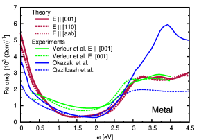
Figure 1: (color online) LDA+CDMFT optical conductivity of the rutile phase of VO₂ for the indicated polarizations ([aab]=[0.85 0.85 0.53]). The velocity matrix elements were calculated using the scheme of Section III.3. Beyond the t_2g orbitals this calculation includes in particular the Ve${}_{g}^{\sigma}$ and O2p orbitals. Experimental curves from (a) PhysRev.172.788 (single crystals, orientation as indicated), (b) qazilbash:205118 (polycrystalline film (T${}_{c}\approx 340$ K), preferential orientation $E\perp[010]$, T=360 K), and (c) PhysRevB.73.165116 (thin film (T${}_{c}\approx 290$ K), $E\perp[001]$, T=300 K).

As one can see, already the three experiments yield quite distinguishable spectra. The differences may point to a polarization dependence, but one cannot rule out an influence of the sample type and the means by which multiple reflections at the sample substrate were treated in case of the thin films. Indeed, in the case of rutile VO₂, x-ray experiments haverkort:196404 witness a rather isotropic response. The different measurements on single crystals PhysRev.172.788 also evidence a quite uniform conductivity up to 4 eV.

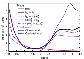
Figure 2: (color online) LDA+CDMFT optical conductivity of rutile VO₂ for the [001] polarization. Shown are the different orbital transitions according to their energy sector, see Eq. (25). The contributions are additive and sum up to the total conductivity. For details see Section III.3. Experimental curves, as above from PhysRevB.73.165116 ; qazilbash:205118 .

The polarization dependence of the theoretical conductivity is found to be rather small, too, which is also in line with our previous statement me_vo2 that the t_2g self-energy shows no particular orbital dependence. Thus, in theory, the metallic Drude-like response is made up from a_1g and e${}_{g}^{\pi}$ density near the Fermi surface.

At higher energies, beyond the Drude-like tail, further inter-“band” intra-t_2g transitions occur. Yet, the optical response is rather structureless up to 2 eV. At this energy, however, we already expect the onset of oxygen 2p derived transitions. In order to elucidate the origin of the spectral weight of this region in greater detail, we plot in Fig. 2 the optical conductivity resolved into the different energy sectors, according to Eq. (25). Since the O2p and the e${}_{g}^{\sigma}$ orbitals were part of the downfolded high energy sector, their position, within our scheme, is frozen to the LDA result (see e.g. the band-structure in eyert_vo2 ). Therefore transitions from the O2p orbitals into the t_2g ones start, as expected, at around 2 eV. We remark that the polarization dependence for the oxygen derived transitions agrees very well with the single crystal experiments PhysRev.172.788 up to 4.5 eV. Transitions from the t_2g orbitals into the e${}_{g}^{\sigma}$ set in later, at around 2.5 eV, and are rather small in magnitude. The O2p to e${}_{g}^{\sigma}$ transitions appear at the expected energies, but they are too low to be seen in Fig. 2.

Overall, the LDA eigenvalues seem to give a rather good description of the e${}_{g}^{\sigma}$ and O2p orbitals, since the agreement with experiment is reasonably accurate, as was qualitatively noticed already in previous LDA optics calculations 0953-8984-19-34-346225 . When looking at photoemission results PhysRevB.43.7263 ; koethe:116402 , one remarks that the on-set of the oxygen 2p is compatible with the LDA, yet, their center of gravity is shifted to slightly higher binding energies in the experiment. As to the e${}_{g}^{\sigma}$ orbitals, it is conceivable, when resorting to x-ray experiments PhysRevB.43.7263 ; koethe:116402 as a reference, that they appear at a little larger energies and with a smaller bandwidth than within the LDA. Of course both comparisons are somewhat indirect, due to the occurrence of matrix elements and other effects in the experiments. Yet, we emphasize that the rather incoherent nature of the t_2g weight in the spectral function me_vo2 is far beyond any band-structure technique, which is why the optical conductivity in the 2.5 to 4.0 eV region, derived from O2p to t_2g transitions, comes out too large in LDA 0953-8984-19-34-346225 when comparing to the experiment of Ref. PhysRev.172.788 , while we find a good agreement for the LDA+CDMFT conductivity.

At this point, we can only speculate on the origin of the shoulder and peak structure seen in one of the experiments qazilbash:205118 at 2.5 eV, and 3.0 eV, see Fig. 2. It seems conceivable that it stems from t_2g to O2p transitions, rather than from e${}_{g}^{\sigma}$ contributions. Attributing the humps to distinct O2p to a_1g or e${}_{g}^{\pi}$ transitions is cumbersome, mostly due to the structure of the numerous oxygen bands. When looking at the momentum-resolved optical conductivity (not shown), one realizes that O2p to e${}_{g}^{\pi}$ transitions start for most of the k-regions at lower energies than transitions into the a_1g.

IV.2 Monoclinic VO₂ – The insulator

We now come to the optical spectra of the monoclinic phase.

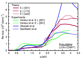
Figure 3: (color online) LDA+CDMFT optical conductivity of the M1 phase of VO₂ for the indicated polarizations ([aab]=[0.84 0.84 0.54]). The velocity matrix elements were calculated using the scheme of Section III.3. Experimental curves from (a) PhysRev.172.788 (single crystals, orientation as indicated), (b) PhysRevB.73.165116 (thin film, $E\perp[001]$, T=280 K), and (c) qazilbash:205118 (polycrystalline film, preferential orientation $E\perp[010]$, T=295 K).

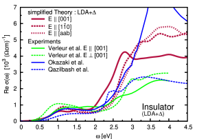
Figure 4: (color online) Optical conductivity of the M1 phase of VO₂ for the indicated polarizations ([aab]=[0.84 0.84 0.54]) when using the effective band-structure me_vo2 “LDA+$\Delta$”. Experimental curves from (a) PhysRev.172.788 (single crystals, orientation as indicated), (b) PhysRevB.73.165116 (thin film, $E\perp[001]$, T=280 K), and (c) qazilbash:205118 (polycrystalline film, preferential orientation $E\perp[010]$, T=295 K)

In Fig. 3 we show our theoretical LDA+CDMFT results, again, in conjunction with the three experiments PhysRev.172.788 ; PhysRevB.73.165116 ; qazilbash:205118 . As was the case for the metallic phase, the latter yield varying results. While the optical gap is roughly 0.5 eV in all cases, the higher energy response is markedly different. Not only the amplitudes, but also the peak positions differ considerably. Yet, as a matter of fact, in the current case of M1 VO₂, a sizable polarization dependence is expected from the structural considerations mentioned above. Indeed our calculation suggests a noticeable anisotropy in the optical response, which is congruent with the experimental findings.

Before interpreting the results, however, we find it instructive to also compute the conductivities using a somewhat simpler approach : In Ref. tomczak_vo2_proc ; me_vo2 we deduced from the LDA+CDMFT self-energies an effective static, yet orbital-dependent, one-particle potential that reproduced the many-body excitation spectrum, which arises when neglecting all life-time effects. Therewith all correlation induced energy shifts are captured, whereas the coherence of the excitations remains infinite. This is equivalent to the use of a scissors operator, albeit one that does not simply widen the gap 0953-8984-19-34-346225 , but selectively shifts the one-particle excitations that mediate the dimerization. We thus replace in a full orbital LDA Hamiltonian the Kohn-Sham eigenvalues of the t_2g orbitals by the ones to which the additional potential was applied, and label the results “LDA+$\Delta$”. For further details see me_vo2 ; me_phd . Therewith, we do not have to invoke the upfolding scheme of Section III.3.

What this theoretical conductivity is missing are the life-time effects encoded in the imaginary part of the LDA+CDMFT self-energy. These were found to be small, yet not entirely negligible me_vo2 . Fig. 3 displays our result, again along with the experimental curves.

When looking first at the optical conductivity that results from the effective band-structure tomczak_vo2_proc ; me_vo2 , “LDA+$\Delta$”, Fig. 4, we find all experimental polarization tendencies reproduced : Consistent with Verleur et al.PhysRev.172.788 , the $E\parallel[001]$ conductivity is lower than the $E\perp[001]$ one at energies up to 1.5 eV, after which the c-axis response develops a little maximum of spectral weight in both, experiment and theory. At energies of 2.35 eV qazilbash:205118 or 3.0 eV PhysRev.172.788 the experimental conductivity with $E\parallel[001]$ components evidences a narrow peak. In the calculation this is prominently seen at 2.75 eV. When looking at our effective band-structure tomczak_vo2_proc ; me_vo2 , it seems plausible that these transitions stem from a_1g bonding to anti-bonding orbitals. The peak is indeed very narrow for an inter-band transition, but in our picture this is simply owing to the fact that the a_1g anti-bonding excitation does exhibit an almost dispersionless behavior tomczak_vo2_proc ; me_vo2 . However, already in this frequency region we expect transitions that involve the oxygen 2p orbitals, as will be detailed below for the LDA+CDMFT conductivity.

At still higher energies, the $E\parallel[001]$ response is again lower than for the perpendicular direction in both, experiment and theory. The overall congruity with experiments further corroborates the validity of our effective band-structure picture for spectral properties and therewith strengthens our interpretation of the nature of the insulating phase of VO₂ as a realization of a “many-body Peierls” state me_vo2 .

Now we compare this simplified approach with the full LDA+CDMFT conductivities of Fig. 3. We instantly realize that the LDA+CDMFT response for the t_2g orbitals is damped and therewith less structured, which was clearly expected. The small underestimation of the optical gap is probably owing to the elevated temperature at which the LDA+CDMFT quantum Monte Carlo calculation was performed biermann:026404 .

To shed further light on the structure of the response, we resolve in Fig. 5 the contributions to the $[001]$ LDA+CDMFT conductivity into their respective energy sectors, according to Section III.3. From this we first infer that the slight upturn, seen for this polarization beyond 1.5 eV in the LDA+CDMFT conductivity is indeed derived from transitions within the t_2g manifold, for oxygen contributions only set in at around 2.0 eV.

Besides, the prominent peak in both, the experimental and LDA+$\Delta$ conductivity with $E\parallel[001]$ polarization that we attributed above to a_1g–a_1g transitions, is largely suppressed and only faintly discernible as a weak shoulder, when comparing with the other polarizations.

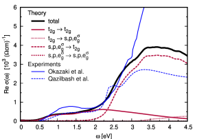
Figure 5: (color online) LDA+CDMFT optical conductivity of M1 VO₂ for the [001] polarization. Shown are the different orbital transitions according to their energy sector, see Eq. (25). The contributions are additive and sum up to the total conductivity. For details see Section III.3. Experimental curve, as above from PhysRevB.73.165116 ; qazilbash:205118 .

As an explanation for this difference between experiment and the approach of the one-particle potential $\Delta$ on the one hand, and the LDA+CDMFT result on the other, we forward the occurrence of sizable life-time effects in the LDA+CDMFT electronic structure calculation. Indeed the a_1g spectral weight in the corresponding t_2g LDA+CDMFT spectral function is not sharply defined and extends over more than 2 eV, and is only barely discernible in the total, orbitally traced, spectrum biermann:026404 . When thinking of the conductivity in simple terms of density-density transitions, it is perfectly conceivable that the a_1g–a_1g response eventuates only in a tail of spectral weight (as seen in the energy sector resolved conductivity in Fig. 5) and not in a well defined peak. Having said this, and referring to the experiments, one might thus conjecture that these life-time effects are still overestimated in the LDA+CDMFT calculation. Moreover, we stress again that the many-body electronic structure was computed at high temperatures biermann:026404 , which will lead to an overestimation of the temperature induced part of the broadening .

Finally, we remark that despite all differences in the experimental data, they reveal (maybe apart from the single crystal for $[001]$ polarization) a common global tendency, namely that, when going from the metal to the insulator, low frequency spectral weight is transfered to higher energies. Indeed, for a given polarization, the Drude-like weight that the insulator is lacking at low energies must be recovered, as requires the f-sum rule millis_review . This condition is met at 5.5 eV in one experiment qazilbash:205118 , while in the other PhysRevB.73.165116 an overcompensation appears already at energies beyond 3.5 eV. Theoretically, when using the LDA+CDMFT conductivity, we find values of 3.73 eV and 4.35 eV, for the $[1\bar{1}0]$ and $[001]$ direction, respectively.

IV.3 Comparison with simpler approaches

In this section we shall briefly show that all the trouble with the Fermi velocity is worth the effort. Therefore we plot in Fig. 6 for the case of M1 VO₂ a comparison of our full scheme, which proved to yield quantitative results, with two simplified calculations. These differ from the full scheme only in the way how the Fermi velocities, i.e. the transition amplitudes are treated. We restrict the discussion to the t_2g response.

To illustrate the effect of the downfolding of orbitals on the matrix elements, we have computed the optical conductivity when applying the generalized Peierls formula on the downfolded Hamiltonian. As we can see, the resulting curves differ considerably from those using the upfolding scheme. In particular, the absolute value for some polarizations is way off with respect to experiment.

It has become a popular approximation to entirely neglect Fermi velocities in the computation of optical properties. Therewith the conductivity is a simple convolution of momentum-resolved spectral functions. As a consequence inter-band transitions are omitted, since the Fermi-velocities are simple unit matrices. Especially in the realistic context this is a severe oversimplification.

Moreover, by construction, there cannot be any orbital dependence in the conductivity, while, as evidenced from the experiments, this is clearly an important issue for M1 VO₂. Also, the magnitude of intra-band transitions is not properly accounted for. In fact, the absolute value of the response is not well defined. In order for this approach to yield a comparable magnitude, we arbitrarily choose a pre-factor : $v_{\mathbf{k}}^{LL^{\prime}}=2r_{0}\delta_{LL^{\prime}}$, with $r_{0}$ being the Bohr radius. As can be inferred from Fig. 6, the resulting peak structure of the optical conductivity is wrong.

Finally, we also compute the optical conductivity when neglecting the multi-atomic correction term in the velocities, i.e. using only the derivative of the Hamiltonian. As was the case for the velocities of the downfolded case, only for one polarization does this yield a reasonable result.

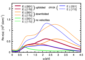
Figure 6: (color online) LDA+CDMFT t_2g optical conductivity of the M1 phase for the indicated polarizations ([aab]=[0.85 0.85 0.53]) and different Fermi velocities. The “upfolded” curves correspond to our full scheme. The “downfolded” data computes the Fermi velocities from the downfolded Hamiltonian. “no velocites” refers to a simple convolution of spectral functions without transition amplitudes. The “dH/dk” curves correspond to neglecting the multi-atomic generalization in the velocities.

V Conclusions

In conclusion we presented a versatile scheme for the calculation of optical properties of correlated materials. Geared at the use with a localized basis set, we devised a realistic extension of the Peierls substitution approach. Moreover, we developed means to incorporate transitions that involve high energy orbitals that were downfolded in the many-body treatment of the electronic structure.

As an application, we evaluated the optical conductivity of VO₂ for both, the metallic and the insulating phase. While the metal is characterized by a rather isotropic response, the insulator revealed a noticeable polarization dependence. The agreement with experiments is overall satisfying. The high energy conductivity is reasonably described when using the LDA band-structure for high lying orbitals. The LDA+CDMFT many-body calculation for the t_2g orbitals correctly describes the low-energy behavior. In the rutile phase it accounts for life-time effects within the t_2g orbitals and therewith also for the damping of oxygen to t_2g transitions with respect to LDA results. In the insulator, it allowed for a genuine reproduction of the experimental t_2g response, capturing in particular the polarization dependence over a wide energy range. The congruity of experiment and theory for the t_2g spectral weight can be interpreted as corroborating the validity of the underlying many-body calculation for the electronic structure along with its interpretation.

Appendix A Continuum formulation of the transition matrix elements

A.1 Derivation of the generalized Peierls velocity in the continuum

Starting from the general Fermi velocity, Eq. (7), which originated from the continuum formulation, we here rederive the generalized Peierls expression as an approximation. The correctional terms contain all intra-atomic transitions, that were completely lacking in the lattice theory, as well as contributions that are owing to the spatial extensions of the wave functions in the solid.

Using $\mathcal{P}_{\alpha}=-{\imath}m/\hbar\left[\mathcal{R}_{\alpha},\hbox{{H}}_{0}\right]$, the element of Eq. (7) can be written

$$\frac{1}{m}\langle\mathbf{k}L^{\prime}|\mathcal{P}_{\alpha}|\mathbf{k}L\rangle=-\frac{{\imath}}{\hbar}\frac{1}{N}\sum_{\mathbf{R},\mathbf{R}^{\prime}}e^{{\imath}\mathbf{k}(\mathbf{R}-\mathbf{R}^{\prime})}\times\qquad$$

$$\int\hbox{d${}^{3}$r }\biggl{[}\langle\hbox{{R}}^{\prime}L^{\prime}|\mathcal{R}_{\alpha}|\hbox{{r}}\rangle\langle\hbox{{r}}|\hbox{{H}}_{0}|\hbox{{R}}L\rangle\bigr{.}\qquad\qquad$$

$$\bigl{.}-\langle\hbox{{R}}^{\prime}L^{\prime}|\hbox{{H}}_{0}|\hbox{{r}}\rangle\langle\hbox{{r}}|\mathcal{R}_{\alpha}|\hbox{{R}}L\rangle\biggr{]}\quad$$ (26)

It is important to note, that here the position operator $\mathcal{R}_{\alpha}$ is defined in the continuum. Its effect in the position representation is $\langle\hbox{{r}}|\mathcal{R}_{\alpha}|\hbox{{R}}L\rangle=r_{\alpha}\chi^{\phantom{*}}_{\mathbf{R}L}(\hbox{{r}})$. This is to be contrasted to the discrete lattice version of Eq. (11). Moreover, one has to make a clear distinction between the continuous space variable r and the discrete unit cell label R. In the (unphysical) limit of completely localized wave functions, $\langle\hbox{{r}}|\hbox{{R}}L\rangle=\chi^{\phantom{*}}_{\mathbf{R}L}(\hbox{{r}})\sim\delta(\hbox{{r}}-\hbox{{R}}_{L})$, this distinction is relaxed, and we recover the expression Eq. (14) of the Peierls approach, as we shall see. Like in the lattice case, we split the atomic positions into $R^{\alpha}_{L}=R^{\alpha}_{\phantom{L}}+\rho_{L}^{\alpha}$. Then the above becomes

$$\frac{1}{m}\langle\mathbf{k}L^{\prime}|\mathcal{P}_{\alpha}|\mathbf{k}L\rangle=-\frac{{\imath}}{\hbar}\frac{1}{N}\sum_{\mathbf{R},\mathbf{R}^{\prime}}e^{{\imath}\mathbf{k}(\mathbf{R}-\mathbf{R}^{\prime})}\times\qquad\qquad$$

$$\biggl{\{}(R_{\alpha}^{\prime}-R_{\alpha}+\rho^{\alpha}_{L^{\prime}}-\rho^{\alpha}_{L})\langle\hbox{{R}}^{\prime}L^{\prime}|\hbox{{H}}_{0}|\hbox{{R}}L\rangle\biggr{.}+$$

$$\int\hbox{d${}^{3}$r }r_{\alpha}\bigl{[}\langle\hbox{{R}}^{\prime}L^{\prime}|\hbox{{r}}+\hbox{{R}}^{\prime}+\mathbf{\rho}_{L^{\prime}}\rangle\langle\hbox{{r}}+\hbox{{R}}^{\prime}+\mathbf{\rho}_{L^{\prime}}|\hbox{{H}}_{0}|\hbox{{R}}L\rangle\bigr{.}$$

$$\qquad\biggl{.}\bigl{.}-\langle\hbox{{R}}^{\prime}L^{\prime}|\hbox{{H}}_{0}|\hbox{{r}}+\hbox{{R}}+\mathbf{\rho}_{L}\rangle\langle\hbox{{r}}+\hbox{{R}}+\mathbf{\rho}_{L}|\hbox{{R}}L\rangle\bigr{]}\biggr{\}}$$ (27)

where we have chosen to condense everything into two different terms. The first one obviously is

$$\frac{1}{\hbar}\biggl{(}\frac{\partial}{\partial k_{\alpha}}\langle\hbox{{k}}L^{\prime}|\hbox{{H}}_{0}|\hbox{{k}}L\rangle-{\imath}(\rho^{\alpha}_{L^{\prime}}-\rho^{\alpha}_{L})\langle\hbox{{k}}L^{\prime}|\hbox{{H}}_{0}|\hbox{{k}}L\rangle\biggr{)}$$ (28)

which is exactly the generalized Peierls expression, Eq. (14). The merit of the Peierls approximation, in particular in realistic calculations, is its apparent simplicity. Indeed no matrix elements other than the Hamiltonian need to be calculated. The latter is a quantity that is anyhow required for a many-body calculation, and one thus has only to perform the directional momentum derivative. From the discussion of the Peierls substitution above, it is clear that the second term in Eq. (27) accounts on the one hand for all atomic transitions ($\hbox{{R}}=\hbox{{R}}^{\prime}$ and $\gamma^{\prime}=\gamma$), yet it also contains contributions that arise from the fact that we started from a continuum formulation. In other words, the spatial extensions of the wave functions lead to inter-atomic, $\gamma^{\prime}\neq\gamma$, corrections, owing to their finite overlap. Yet, a direct evaluation of these terms is an intricate undertaking, since it involves the calculation of many integrals. Therefore, it is a valid question whether the generalization of the Peierls approach, as such, already gives a reasonable approximation, without considering the terms beyond it, and if so, under which circumstances. Though the regrouping of terms into the Peierls expression and the rest was guided from the lattice considerations, it might still seem somewhat arbitrary. The next section however reveals that the intuition of an increased validity of the Peierls approach with a better localization of the involved orbitals is actually warranted.

A.2 The Peierls substitution as the localized limit

In the following, we will make consecutive approximations regarding the extension of the orbitals, which lead, step by step, to more simplified correction terms to the Peierls expression Eq. (28), which one might endeavor to take into account in an actual computation. Moreover, these approximative steps will rationalize the identification of the Peierls term as the leading contribution to the Fermi velocities in the considered setup.

By assuming well localized orbitals, we thus proceed to cut down the expression in question to the predominant terms, which will be given by the integrals that involve wave functions that have a large overlap . Indeed, we show that in the limit of perfect localization (or equivalently in the limit of large atomic separation) the only surviving transition elements are given by the intra-atomic contributions, that were missing in the Peierls formulation. Using $\langle\hbox{{r}}+\hbox{{R}}|\hbox{{R}}L\rangle=\chi^{\phantom{*}}_{\mathbf{R}L}(\hbox{{r}}+\hbox{{R}})=\chi^{\phantom{*}}_{\mathbf{0}L}(\hbox{{r}})$, the terms beyond the Peierls ones can be put into the form

$$-\frac{{\imath}}{\hbar}\frac{1}{N}\sum_{\mathbf{R},\mathbf{R}^{\prime}}e^{{\imath}\mathbf{k}(\mathbf{R}-\mathbf{R}^{\prime})}\int\hbox{d${}^{3}$r }r_{\alpha}\sum_{\mathbf{\Lambda},L^{\prime\prime}}$$ (29)

$$\biggl{[}\chi_{\mathbf{0}L^{\prime}}^{*}(\hbox{{r}}+\mathbf{\rho}_{L^{\prime}})\chi^{\phantom{*}}_{\mathbf{0}L^{\prime\prime}}(\hbox{{r}}+\hbox{{R}}^{\prime}-\mathbf{\Lambda}+\mathbf{\rho}_{L^{\prime}})\langle\mathbf{\Lambda}L^{\prime\prime}|\hbox{{H}}_{0}|\hbox{{R}}L\rangle\biggr{.}$$

$$-\biggl{.}\chi_{\mathbf{0}L^{\prime\prime}}^{*}(\hbox{{r}}+\hbox{{R}}-\mathbf{\Lambda}+\mathbf{\rho}_{L})\chi^{\phantom{*}}_{\mathbf{0}L}(\hbox{{r}}+\mathbf{\rho}_{L})\langle\hbox{{R}}^{\prime}L^{\prime}|\hbox{{H}}_{0}|\mathbf{\Lambda}L^{\prime\prime}\rangle\biggr{]}$$

In this formula the origins of all intervening wave functions lie within the same unit cell, labeled “0” . In a first step, the assumed localization of the involved orbitals makes it reasonable to identify important terms in the sum as those, where the arguments of the wave functions also lie within the same unit cell, i.e. $\mathbf{\Lambda}=\hbox{{R}}^{\prime}$ in the first term and $\mathbf{\Lambda}=\hbox{{R}}$ in the second one. We note that within this approximation, only the Hamiltonian element depends on the unit cell labels R and $\hbox{{R}}^{\prime}$, and we can thus directly perform the Fourier transformation, yielding

$$-\frac{{\imath}}{\hbar}\int\hbox{d${}^{3}$r }r_{\alpha}\sum_{L^{\prime\prime}}$$ (30)

$$\quad\biggl{[}\chi_{\mathbf{0}L^{\prime}}^{*}(\hbox{{r}}+\mathbf{\rho}_{L^{\prime}})\chi^{\phantom{*}}_{\mathbf{0}L^{\prime\prime}}(\hbox{{r}}+\mathbf{\rho}_{L^{\prime}})\langle\hbox{{k}}L^{\prime\prime}|\hbox{{H}}_{0}|\hbox{{k}}L\rangle\biggr{.}$$

$$\qquad-\biggl{.}\chi_{\mathbf{0}L^{\prime\prime}}^{*}(\hbox{{r}}+\mathbf{\rho}_{L})\chi^{\phantom{*}}_{\mathbf{0}L}(\hbox{{r}}+\mathbf{\rho}_{L})\langle\hbox{{k}}L^{\prime}|\hbox{{H}}_{0}|\hbox{{k}}L^{\prime\prime}\rangle\biggr{]}$$

This means that the entire momentum dependence, in this approximation, is carried by the Hamiltonian. The complexity of the occurring matrix elements of the position operator has been considerably reduced. In the one-atomic case, i.e. $\gamma=\gamma^{\prime}=\gamma^{\prime\prime}$, and when using the short-hand notation $\hbox{{R}}_{\alpha,0}^{LL^{\prime}}=\langle\hbox{{0}}L|\mathcal{R}_{\alpha}|\hbox{{0}}L^{\prime}\rangle$, $\hbox{{H}}_{0}^{LL^{\prime}}(\hbox{{k}})=\langle\hbox{{k}}L|\hbox{{H}}_{0}|\hbox{{k}}L^{\prime}\rangle$ we simply have

$$-\frac{{\imath}}{\hbar}\left[\hbox{{R}}_{\alpha,0},\hbox{{H}}_{0}(\hbox{{k}})\right]_{L^{\prime}L}$$ (31)

This is reminiscent of the relation $1/m\mathcal{P}=-{\imath}/\hbar\left[\mathcal{R},\hbox{{H}}_{0}\right]$, which we used in the beginning. Here however intervene on-site matrix elements rather than the full position operator. Indeed these elements, $\hbox{{R}}_{\alpha,0}^{LL^{\prime}}$, are well known in atomic physics : They give the usual amplitudes for atomic dipolar transitions : The angular part of the integral will produce the corresponding dipole selection rules ($\Delta l=\pm 1,\Delta m=0,\pm 1$) via Clebsch-Gordon coefficients (see e.g. tannoudji ), when, as we have assumed, the wave functions have a well-defined angular momentum $(l,m)$. Contrary to the atomic case, however, the Hamiltonian is momentum dependent, owing to the fact that, though regarding atomic transitions, the “atom” is here embedded in a solid. Also, the above term reminds the form of the multi-atomic correction term in Eq. (28), only that there occurred fixed atomic positions $\mathbf{\rho}_{\gamma}$, which commute with the Hamiltonian, which is why in Eq. (28) only the non-local terms $\gamma\neq\gamma^{\prime}$ appear.

Coming back to the multi-atomic case, we have to make a further approximation in order to obtain an expression containing atomic transitions only. Yet, the shifts in the wave functions of Eq. (30) can be treated analogous to the unit cell coordinates : Indeed $\chi^{\phantom{*}}_{\mathbf{0}L}(\hbox{{r}}+\mathbf{\rho}_{L})$ is centered around the position of atom $\gamma$. When, for the sake of clarity, we rename $\widetilde{\chi}^{\phantom{*}}_{\mathbf{0}L}(\hbox{{r}})=\chi^{\phantom{*}}_{\mathbf{0}L}(\hbox{{r}}+\mathbf{\rho}_{L})$ we find

$$-\frac{{\imath}}{\hbar}\int\hbox{d${}^{3}$r }r_{\alpha}\sum_{L^{\prime\prime}}$$ (32)

$$\quad\biggl{[}\widetilde{\chi}_{\mathbf{0}L^{\prime}}^{*}(\hbox{{r}})\widetilde{\chi}^{\phantom{*}}_{\mathbf{0}L^{\prime\prime}}(\hbox{{r}}+\mathbf{\rho}_{L^{\prime}}-\mathbf{\rho}_{L^{\prime\prime}})\langle\hbox{{k}}L^{\prime\prime}|\hbox{{H}}_{0}|\hbox{{k}}L\rangle\biggr{.}$$

$$\qquad-\biggl{.}\widetilde{\chi}_{\mathbf{0}L^{\prime\prime}}^{*}(\hbox{{r}}+\mathbf{\rho}_{L}-\mathbf{\rho}_{L^{\prime\prime}})\widetilde{\chi}^{\phantom{*}}_{\mathbf{0}L}(\hbox{{r}})\langle\hbox{{k}}L^{\prime}|\hbox{{H}}_{0}|\hbox{{k}}L^{\prime\prime}\rangle\biggr{]}$$

From this expression it is plausible, that for localized orbitals atomic transitions ($\gamma^{\prime\prime}=\gamma^{\prime}$ and $\gamma^{\prime\prime}=\gamma$, respectively) are in fact predominant. When restraining ourselves to these cases, we thus drop entirely the corrections to hopping processes that stem from the finite extensions of the wave-functions and end up with

$$-\frac{{\imath}}{\hbar}\int\hbox{d${}^{3}$r }r_{\alpha}\left[\sum_{L^{\prime\prime}}^{\gamma^{\prime\prime}=\gamma^{\prime}}\widetilde{\chi}_{\mathbf{0}L^{\prime}}^{*}(\hbox{{r}})\widetilde{\chi}^{\phantom{*}}_{\mathbf{0}L^{\prime\prime}}(\hbox{{r}})\langle\hbox{{k}}L^{\prime\prime}|\hbox{{H}}_{0}|\hbox{{k}}L\rangle\right.$$ (33)

$$\left.-\sum_{L^{\prime\prime}}^{\gamma^{\prime\prime}=\gamma}\widetilde{\chi}_{\mathbf{0}L^{\prime\prime}}^{*}(\hbox{{r}})\widetilde{\chi}^{\phantom{*}}_{\mathbf{0}L}(\hbox{{r}})\langle\hbox{{k}}L^{\prime}|\hbox{{H}}_{0}|\hbox{{k}}L^{\prime\prime}\rangle\right]$$

$$= -\frac{{\imath}}{\hbar}\left[\sum_{L^{\prime\prime}}^{\gamma^{\prime\prime}=\gamma^{\prime}}\langle\widetilde{\hbox{{0}}L^{\prime}}|\mathcal{R}_{\alpha}|\widetilde{\hbox{{0}}L^{\prime\prime}}\rangle\langle\hbox{{k}}L^{\prime\prime}|\hbox{{H}}_{0}|\hbox{{k}}L\rangle\right.$$

$$\left.-\sum_{L^{\prime\prime}}^{\gamma^{\prime\prime}=\gamma}\langle\widetilde{\hbox{{0}}L^{\prime\prime}}|\mathcal{R}_{\alpha}|\widetilde{\hbox{{0}}L}\rangle\langle\hbox{{k}}L^{\prime}|\hbox{{H}}_{0}|\hbox{{k}}L^{\prime\prime}\rangle\right]$$

Here, only the terms in which the Hamiltonian element is diagonal in the atomic index $\gamma$ can be written in the form of a commutator, as was the case in the one-atomic case in Eq. (31). In total, the above term contains intra-atomic transitions only. These were completely missing in the Peierls approach, as explained above. Under the assumptions on the localization of the involved orbitals, the Peierls term, Eq. (28), thus turns out to be the most important contribution to the Fermi velocity. Intuitively, this approach is thus particularly suited for systems in which e.g. 3d or 4f orbitals play an important role, since these verify the request of a high degree of localization.

Another point, worth noticing, is the fact, that, when using the Peierls approximation, the result of the conductivity is actually basis dependent. It is the momentum derivative of the Hamiltonian, which constitutes the first term in Eq. (28), that transforms evidently differently than the Hamiltonian itself. Obviously this is an artifact of the approximations from which the Peierls expression eventuated. Since, however, the term corresponds to the limit of perfect localization, it is expected to still yield reasonable results for orbitals that are short-ranged. We will come back to this in the next paragraph, in the context of Fermi velocities for downfolded Hamiltonians.

Improvements to the above approximations are obvious: One could e.g. take into account elements containing nearest-neighbor wave functions within the same unit cell, or even account for wave functions centered in different unit cells. An evaluation of these terms in principle allows for a more quantitative assessment of the quality of the Peierls term. However, the matrix elements that one needs to evaluate are numerous and more complex since they explicitly involve various wave functions. We stress again, that these terms are inter-atomic corrections to the Peierls term, while the intra-atomic contributions are absent in the Peierls formalism by construction, and given by Eq. (33).

References

- (1) K. Okazaki, S. Sugai, Y. Muraoka, and Z. Hiroi. Role of electron-electron and electron-phonon interaction effects in the optical conductivity of VO2. Phys. Rev. B, 73(16):165116, Apr 2006.
- (2) A. Zimmers, J. M. Tomczak, R. P. S. M. Lobo, N. Bontemps, C. P. Hill, M. C. Barr, Y. Dagan, R. L. Greene, A. J. Millis, and C. C. Homes. Infrared properties of electron-doped cuprates: Tracking normal-state gaps and quantum critical behavior in Pr2-xCexCuO4. Europhys. Lett., 70(2):225–231, 2005.
- (3) M. M. Qazilbash, M. Brehm, Byung-Gyu Chae, P.-C. Ho, G. O. Andreev, Bong-Jun Kim, Sun Jin Yun, A. V. Balatsky, M. B. Maple, F. Keilmann, Hyun-Tak Kim, and D. N. Basov. Mott Transition in VO2 Revealed by Infrared Spectroscopy and Nano-Imaging. Science, 318(5857):1750–1753, 2007.
- (4) L. Baldassarre, A. Perucchi, D. Nicoletti, A. Toschi, G. Sangiovanni, K. Held, M. Capone, M. Ortolani, L. Malavasi, M. Marsi, P. Metcalf, P. Postorino, and S. Lupi. Quasiparticle evolution and pseudogap formation in V2O3: An infrared spectroscopy study. Phys. Rev. B, 77(11):113107, 2008.
- (5) S.S.A. Seo J.S. Kim P. Popovich Y. Matiks R.K. Kremer B. Keimer A.V. Boris, N.N. Kovaleva. Signatures of electronic correlations in optical properties of lafeaso1-xfx. (arXiv:0806.1732), 2008.
- (6) W. Kohn. Nobel lecture: Electronic structure of matter-wave functions and density functionals. Rev. Mod. Phys., 71(5):1253–1266, Oct 1999.
- (7) W. Kohn and L. J. Sham. Self-consistent equations including exchange and correlation effects. Phys. Rev., 140(4A):A1133–A1138, Nov 1965.
- (8) L. Hedin. New method for calculating the one-particle green’s function with application to the electron-gas problem. Phys. Rev., 139(3A):A796–A823, Aug 1965.
- (9) A. Georges, G. Kotliar, W. Krauth, and M. J. Rozenberg. Dynamical mean-field theory of strongly correlated fermion systems and the limit of infinite dimensions. Rev. Mod. Phys., 68(1):13, Jan 1996.
- (10) G. Kotliar and D. Vollhardt. Strongly correlated materials: Insights from dynamical mean-field theory. Physics Today, 57(3):53, 2004.
- (11) K. Held, I. A. Nekrasov, G. Keller, V. Eyert, N. Blümer, A. K. McMahan, R. T. Scalettar, Th. Pruschke, V. I. Anisimov, and D. Vollhardt. Realistic investigations of correlated electron systems within lda+dmft. Psi-k Newsletter, 56(65), 2003.
- (12) S. Biermann. Lda+dmft - a tool for investigating the electronic structure of materials with strong electronic coulomb correlations. in Encyclopedia of Materials: Science and Technology, 2006.
- (13) F. J. Morin. Oxides which show a metal-to-insulator transition at the neel temperature. Phys. Rev. Lett., 3(1):34–36, Jul 1959.
- (14) J. P. Pouget and H. Launois. Metal insulator phase transition in vo2. J.Phys. France, 37:C4–49, 1976.
- (15) John B. Goodenough. Direct cation- -cation interactions in several oxides. Phys. Rev., 117(6):1442–1451, Mar 1960.
- (16) J. B. Goodenough. The two components of the crystallographic transition in vo2. J. Solid State Chem., 3:490–500, Mar 1971.
- (17) R. E. Peierls. Quantum Theory of Solids. Clarendon, Oxford, 1955.
- (18) A. Zylbersztejn and N. F. Mott. Metal-insulator transition in vanadium dioxide. Phys. Rev. B, 11(11):4383–4395, Jun 1975.
- (19) J. P. Pouget, H. Launois, J. P. D’Haenens, P. Merenda, and T. M. Rice. Electron localization induced by uniaxial stress in pure vo2. Phys. Rev. Lett., 35(13):873–875, Sep 1975.
- (20) J. P. Pouget, H. Launois, T. M. Rice, P. Dernier, A. Gossard, G. Villeneuve, and P. Hagenmuller. Dimerization of a linear heisenberg chain in the insulating phases of . Phys. Rev. B, 10(5):1801–1815, Sep 1974.
- (21) T. C. Koethe, Z. Hu, M. W. Haverkort, C. Schussler-Langeheine, F. Venturini, N. B. Brookes, O. Tjernberg, W. Reichelt, H. H. Hsieh, H.-J. Lin, C. T. Chen, and L. H. Tjeng. Transfer of spectral weight and symmetry across the metal-insulator transition in vo2. Phys. Rev. Lett., 97(11):116402, 2006.
- (22) M. W. Haverkort, Z. Hu, A. Tanaka, W. Reichelt, S. V. Streltsov, M. A. Korotin, V. I. Anisimov, H. H. Hsieh, H.-J. Lin, C. T. Chen, D. I. Khomskii, and L. H. Tjeng. Orbital-assisted metal-insulator transition in vo2. Phys. Rev. Lett., 95(19):196404, 2005.
- (23) R. Eguchi, M. Taguchi, M. Matsunami, K. Horiba, K. Yamamoto, Y. Ishida, A. Chainani, Y. Takata, M. Yabashi, D. Miwa, Y. Nishino, K. Tamasaku, T. Ishikawa, Y. Senba, H. Ohashi, Y. Muraoka, Z. Hiroi, and S. Shin. Photoemission evidence for a mott-hubbard metal-insulator transition in vo[sub 2]. Phys. Rev. B, 78(7):075115, 2008.
- (24) M. M. Qazilbash, M. Brehm, G. O. Andreev, A. Frenzel, P.-C. Ho, Byung-Gyu Chae, Bong-Jun Kim, Sun Jin Yun, Hyun-Tak Kim, A. V. Balatsky, O. G. Shpyrko, M. B. Maple, F. Keilmann, and D. N. Basov. Infrared spectroscopy and nano-imaging of the insulator-to-metal transition in vanadium dioxide. Phys. Rev. B, 79(7):075107, 2009.
- (25) L. A. Ladd and William Paul. Optical and transport properties of high quality crystals of near the metallic transition temperature. Solid State Commun., 7:425–428, 1969.
- (26) R. M. Wentzcovitch, W. W. Schulz, and P. B. Allen. : Peierls or mott-hubbard? a view from band theory. Phys. Rev. Lett., 72(21):3389–3392, May 1994.
- (27) V. Eyert. The metal-insulator transitions of vo2: A band theoretical approach. Ann. Phys. (Leipzig), 11:650, 2002.
- (28) M. A. Korotin, N. A. Skorikov, and V. I. Anisimov. Phys. Met. Metallogr., 94(1):17, 2002.
- (29) M. Imada, A. Fujimori, and Y. Tokura. Metal-insulator transitions. Rev. Mod. Phys., 70(4):1039–1263, Oct 1998.
- (30) Jan M. Tomczak. Spectral and Optical Properties of Correlated Materials. PhD thesis, Ecole Polytechnique, France, 2007.
- (31) M. S. Laad, L. Craco, and E. Müller-Hartmann. Vo2: A two-fluid incoherent metal? Europhys. Lett., 69(6):984–989, 2005.
- (32) A. Liebsch, H. Ishida, and G. Bihlmayer. Coulomb correlations and orbital polarization in the metal-insulator transition of vo2. Phys. Rev. B, 71(8):085109, 2005.
- (33) S. Biermann, A. Poteryaev, A. I. Lichtenstein, and A. Georges. Dynamical singlets and correlation-assisted peierls transition in vo2. Phys. Rev. Lett., 94(2):026404, 2005.
- (34) J. M. Tomczak and S. Biermann. Effective band structure of correlated materials: the case of vo2. J. Phys.: Cond. Matter, 19(36):365206, 2007.
- (35) Jan M. Tomczak, Ferdi Aryasetiawan, and Silke Biermann. Effective bandstructure in the insulating phase versus strong dynamical correlations in metallic vo2. Phys. Rev. B, 78(11):115103, 2008.
- (36) A. Continenza, S. Massidda, and M. Posternak. Self-energy corrections in within a model scheme. Phys. Rev. B, 60(23):15699–15704, Dec 1999.
- (37) R. Sakuma, T. Miyake, and F. Aryasetiawan. First-principles study of correlation effects in vo[sub 2]. Phys. Rev. B, 78(7):075106, 2008.
- (38) Matteo Gatti, Fabien Bruneval, Valerio Olevano, and Lucia Reining. Understanding correlations in vanadium dioxide from first principles. Phys. Rev. Lett., 99(26):266402, 2007.
- (39) Ulrich Eckern Xiangyang Huang, Weidong Yang. Metal-insulator transition in vo2: a peierls-mott-hubbard mechanism. (arXiv:cond-mat/9808137), 1998.
- (40) A. Tanaka. A new scenario on the metal-insulator transition in vo2. J. Phys. Soc. Jpn., 72(10):2433, 2003.
- (41) R.J.O. Mossanek and M. Abbate. Evolution of the d[short parallel] band across the metal-insulator transition in vo2. Solid State Communications, 135(3):189 – 192, 2005.
- (42) R. J. O. Mossanek and M. Abbate. Cluster model calculations with nonlocal screening channels of metallic and insulating vo[sub 2]. Phys. Rev. B, 74(12):125112, 2006.
- (43) A. S. Barker, H. W. Verleur, and H. J. Guggenheim. Infrared optical properties of vanadium dioxide above and below the transition temperature. Phys. Rev. Lett., 17(26):1286–1289, Dec 1966.
- (44) Hans W. Verleur, A. S. Barker, and C. N. Berglund. Optical properties of v between 0.25 and 5 ev. Phys. Rev., 172(3):788–798, Aug 1968.
- (45) S. Shin, S. Suga, M. Taniguchi, M. Fujisawa, H. Kanzaki, A. Fujimori, H. Daimon, Y. Ueda, K. Kosuge, and S. Kachi. Vacuum-ultraviolet reflectance and photoemission study of the metal-insulator phase transitions in , , and . Phys. Rev. B, 41(8):4993–5009, Mar 1990.
- (46) M. Abbate, F. M. F. de Groot, J. C. Fuggle, Y. J. Ma, C. T. Chen, F. Sette, A. Fujimori, Y. Ueda, and K. Kosuge. Soft-x-ray-absorption studies of the electronic-structure changes through the phase transition. Phys. Rev. B, 43(9):7263–7266, Mar 1991.
- (47) G. A. Sawatzky and D. Post. X-ray photoelectron and auger spectroscopy study of some vanadium oxides. Phys. Rev. B, 20(4):1546–1555, Aug 1979.
- (48) M. M. Qazilbash, K. S. Burch, D. Whisler, D. Shrekenhamer, B. G. Chae, H. T. Kim, and D. N. Basov. Correlated metallic state of vanadium dioxide. Phys. Rev. B, 74(20):205118, 2006.
- (49) M. M. Qazilbash, A. A. Schafgans, K. S. Burch, S. J. Yun, B. G. Chae, B. J. Kim, H. T. Kim, and D. N. Basov. Electrodynamics of the vanadium oxides vo2 and v2o3. Phys. Rev. B, 77(11):115121, 2008.
- (50) Byung-Gyu Chae, Hyun-Tak Kim, Sun-Jin Yun, Bong-Jun Kim, Yong-Wook Lee, Doo-Hyeb Youn, and Kwang-Yong Kang. Highly oriented vo2 thin films prepared by sol-gel deposition. Electrochemical and Solid-State Letters, 9(1):C12–C14, 2006.
- (51) O. Gunnarsson, M. Calandra, and J. E. Han. Colloquium: Saturation of electrical resistivity. Rev. Mod. Phys., 75(4):1085–1099, Oct 2003.
- (52) Anibal Gavini and Clarence C. Y. Kwan. Optical properties of semiconducting v films. Phys. Rev. B, 5(8):3138–3143, Apr 1972.
- (53) R J O Mossanek and M Abbate. Optical response of metallic and insulating vo2 calculated with the lda approach. J. Phys.: Cond. Matter, 19(34):346225 (10pp), 2007.
- (54) Th. Pruschke, D. L. Cox, and M. Jarrell. Hubbard model at infinite dimensions: Thermodynamic and transport properties. Phys. Rev. B, 47(7):3553–3565, Feb 1993.
- (55) M. Jarrell, J. K. Freericks, and Th. Pruschke. Optical conductivity of the infinite-dimensional hubbard model. Phys. Rev. B, 51(17):11704–11711, May 1995.
- (56) M. J. Rozenberg, G. Kotliar, H. Kajueter, G. A. Thomas, D. H. Rapkine, J. M. Honig, and P. Metcalf. Optical conductivity in mott-hubbard systems. Phys. Rev. Lett., 75(1):105–108, Jul 1995.
- (57) M. J. Rozenberg, G. Kotliar, and H. Kajueter. Transfer of spectral weight in spectroscopies of correlated electron systems. Phys. Rev. B, 54(12):8452–8468, Sep 1996.
- (58) N. Blümer. Mott-Hubbard Metal-Insulator Transition and Optical Conductivity in High Dimensions. PhD thesis, Universität Augsburg, 2002.
- (59) N. Blümer and P. G. J. van Dongen. Transport properties of correlated electrons in high dimensions, 2003.
- (60) G. Pálsson. Computational studies of thermoelectricity in strongly correlated electron systems. PhD thesis, Rutgers, The State University of New Jersey, 2001.
- (61) E Pavarini, A Yamasaki, J Nuss, and O K Andersen. How chemistry controls electron localization in 3d1 perovskites: a wannier-function study. New Journal of Physics, 7:188, 2005.
- (62) A. Perlov, S. Chadov, and H. Ebert. Green function approach for the ab initio calculation of the optical and magneto-optical properties of solids: Accounting for dynamical many-body effects. Phys. Rev. B, 68(24):245112, Dec 2003.
- (63) V. S. Oudovenko, G. Palsson, S. Y. Savrasov, K. Haule, and G. Kotliar. Calculations of optical properties in strongly correlated materials. Phys. Rev. B, 70(12):125112, 2004.
- (64) J. M. Tomczak and S. Biermann. Multi-orbital effects in optical properties of vanadium sesquioxide. J. Phys.: Cond. Matter, 21(064209), 2009.
- (65) Alexander I. Poteryaev, Jan M. Tomczak, Silke Biermann, Antoine Georges, Alexander I. Lichtenstein, Alexey N. Rubtsov, Tanusri Saha-Dasgupta, and Ole K. Andersen. Enhanced crystal-field splitting and orbital-selective coherence induced by strong correlations in v2o3. Phys. Rev. B, 76(8):085127, 2007.
- (66) J. M. Tomczak and S. Biermann. Materials design using correlated oxides: Optical properties of vanadium dioxide. 2009. Europhys. Lett. accepted, preprint: arXiv:0807.4044.
- (67) Jan M. Tomczak and S. Biermann. Optical properties of correlated materials - or why intelligent windows may look dirty. Scientific Highlight of the Month, August(88), 2008.
- (68) Gerald D. Mahan. Many-particle Physics. Plenum Press, 1990.
- (69) P. Coleman. The evolving monogram on Many Body Physics. 2004.
- (70) Anil Khurana. Electrical conductivity in the infinite-dimensional hubbard model. Phys. Rev. Lett., 64(16):1990, Apr 1990.
- (71) O. Krogh Andersen. Linear methods in band theory. Phys. Rev. B, 12(8):3060–3083, Oct 1975.
- (72) O. K. Andersen and T. Saha-Dasgupta. Muffin-tin orbitals of arbitrary order. Phys. Rev. B, 62(24):R16219–R16222, Dec 2000.
- (73) F. Lechermann, A. Georges, A. Poteryaev, S. Biermann, M. Posternak, A. Yamasaki, and O. K. Andersen. Dynamical mean-field theory using wannier functions: A flexible route to electronic structure calculations of strongly correlated materials. Phys. Rev. B, 74(12):125120, 2006.
- (74) R. Peierls. Z. Physik, 80:763, 1933.
- (75) A. J. Millis. Optical conductivity and correlated electron physics. In L. Degiorgi D. Baeriswyl, editor, Strong Interactions in Low Dimensions, volume 25, page 195ff. Physics and Chemistry of Materials with Low-Dimensional Structures, 2004.
- (76) V. I. Anisimov, D. E. Kondakov, A. V. Kozhevnikov, I. A. Nekrasov, Z. V. Pchelkina, J. W. Allen, S.-K. Mo, H.-D. Kim, P. Metcalf, S. Suga, A. Sekiyama, G. Keller, I. Leonov, X. Ren, and D. Vollhardt. Full orbital calculation scheme for materials with strongly correlated electrons. Phys. Rev. B, 71(12):125119, 2005.
- (77) F. Aryasetiawan, J. M. Tomczak, T. Miyake, and R. Sakuma. Downfolded self-energy of many-electron systems. 2009. Phys. Rev. Lett. accepted, preprint: arXiv:0806.3373.
- (78) C. Cohen-Tannoudji, B. Diu, and F. Laloë. Mécanique quantique. Hermann, 1992.