Analytic Aperture Calculation and Scaling Laws for Radio Detection of Lunar-Target UHE Neutrinos

Abstract

We derive analytic expressions, and approximate them in closed form, for the effective detection aperture for Cerenkov radio emission from ultra-high-energy neutrinos striking the Moon. The resulting apertures are in good agreement with recent Monte Carlo simulations and support the conclusion of James & Protheroe (2009) that neutrino flux upper limits derived from the GLUE search (Gorham et al., 2004) were too low by an order of magnitude. We also use our analytic expressions to derive scaling laws for the aperture as a function of observational and lunar parameters. We find that at low frequencies downward-directed neutrinos always dominate, but at higher frequencies, the contribution from upward-directed neutrinos becomes increasingly important, especially at lower neutrino energies. Detecting neutrinos from Earth near the GZK regime will likely require radio telescope arrays with extremely large collecting area ($A_{e}\sim 10^{6}$ m²) and hundreds of hours exposure time. Higher energy neutrinos are most easily detected using lower frequencies. Lunar surface roughness is a decisive factor for obtaining detections at higher frequencies ($\nu\mathrel{\hbox to0.0pt{\lower 3.0pt\hbox{$\mathchar 536\relax$}\hss}\raise 2.0pt\hbox{$\mathchar 318\relax$}}$ 300 MHz) and higher energies ($E\mathrel{\hbox to0.0pt{\lower 3.0pt\hbox{$\mathchar 536\relax$}\hss}\raise 2.0pt\hbox{$\mathchar 318\relax$}}10^{21}$ eV).

1 Introduction

The ubiquitous presence of ultra-high-energy (UHE, $E_{\nu}>10^{18}$ eV) cosmic rays suggests the existence of an equally ubiquitous and similarly high-energy cosmic neutrino population, either as a result of the various mechanisms for generating muon neutrinos from charged pion decay in the vicinity of the cosmic-ray acceleration region (Bahcall & Waxman, 2001), or during interactions with the cosmic background radiation (GZK effect, Greisen, 1966; Zatsepin & Kuz’min, 1966). One effort to detect such neutrinos involves radio observations of the expected Cerenkov burst emission when these neutrinos interact with the Moon. Several experiments have already attempted to detect this signal (e.g., Hankins et al., 1996; Gorham et al., 2004; Beresnyak et al., 2005; Buitink et al., 2008) all with null results to date. But even null results can be converted into useful upper bounds for the UHE neutrino flux, provided that the effective aperture, the area times the solid angle through which incident neutrinos are detectable, is known.

For future experiments, it is clear that the larger the aperture, the greater will be the possibility of achieving a detection, or the more decisively constraining will be the inferred upper limit. Of particular note is the fact that all the experiments so far have suffered from particularly weak coverage of the energy domain near the GZK cutoff near $10^{19.6}$ eV, the region of perhaps the highest cosmological interest, and also possibly a local peak in the neutrino spectrum. The poor coverage is largely due to inherent limitations on radio observations, but it may also in part be due to the difficulty in achieving optimal tailoring of the observing parameters. Having access to closed-form expressions of general validity would yield not only a convenient means for calculating the aperture, it would also assist in such optimization of experimental design, for penetrating deeper into this hitherto uncharted neutrino regime.

Despite their potential value, no such closed-form expressions are currently available in the literature, and so the primary purpose of this paper is to provide such expressions. We then apply them to the question of how to optimize for detection of GZK and other UHE neutrinos by looking for radio Cerenkov signals from the Moon. The approach is general enough for future modifications to accommodate other types of experiments, such as terrestrial ice sheets seen from airborne balloons, or the Moon seen from lunar orbit.

To account for the neutrino properties and their detectability in closed-form aperture expressions, we rely on previous determinations of the basic attributes of radio Cerenkov emission from ultra-high-energy (UHE) hadronic showers (e.g., James & Protheroe, 2009) and reviews of the basic physics of the Askar’yan effect, whereby neutrinos generate charge excesses in hadronic showers (e.g., Alvarez-Muniz & Zas, 2001). Here we will not comment on these physical processes, but merely quote the results from the literature as we apply them to our specific problem.

In this paper we assume that all contributing neutrino showers occur in the lunar regolith near the surface, with a fixed index of refraction of $n_{r}=1.73$ (James & Protheroe, 2009), so we ignore inhomogeneities such as the sub-regolith. James & Protheroe (2009) have evaluated a sub-regolith contribution and find that it can only significantly increase the aperture for Earthbound detection at very high neutrino energies ($E\mathrel{\hbox to0.0pt{\lower 3.0pt\hbox{$\mathchar 536\relax$}\hss}\raise 2.0pt\hbox{$\mathchar 318\relax$}}10^{22}$ eV), because only such high-energy neutrinos produce sufficiently strong fields to be above the minimum detectable level at the surface. Of course, experiments from a closer distance, such as lunar orbiters like LORD (Gusev et al., 2006), could receive significant contributions from the sub-regolith, and ignoring gradients in the lunar material introduces potential errors but is certainly a greatly simplifying assumption.

2 General form of the aperture calculation

Our goal is to determine the rate of detection of hadronic showers initiated in the Moon by the capture of a high-energy cosmic neutrino, via the detection of the resulting radio-frequency electric fields propagating from the Moon. One way to conceptualize this detection rate is in terms of an aperture size, which when multiplied by the incident neutrino flux in each energy bin of interest, gives the detection rate in that bin. Since the diffuse neutrino background flux is scaled per area and per solid angle, the aperture will be in units of an area times a solid angle (Williams, 2004).

Our approach for analytically specifying this aperture begins with identifying the maximum possible aperture ${A_{max}}$ that an amount of mass equivalent to the lunar mass could possibly achieve, assuming that each neutrino interacting with that material is detected exactly once. Note this would actually require the lunar material be unphysically spread out, among other impossible requirements. Thus it is merely a starting point, and it follows clearly that

$${A_{max}}(E)=4\pi M\kappa(E)$$ (1)

for mass $M$ (of the Moon) exhibiting a cross section per gram $\kappa(E)$ for initiating charged particle showers for neutrinos at energy $E$, incident over the full 4$\pi$ steradians of sky.

Our approach is then to reduce the aperture by eliminating events that are blocked from occuring by virtue of prior absorption of the neutrino elsewhere in the spherical Moon, and then reduce it further by requiring that the events yield radio signals above the detection threshold of the specified telescope system along some ray that intersects the detector. These reductions are substantial for three reasons: ultra-high-energy (UHE) neutrinos are drastically truncated by the opaqueness of the Moon, total internal reflection at the lunar surface reduces the rays that successfully cross the falling refractive index at this boundary, and rays from depth in the Moon are significantly attenuated by lunar radio absorption. The remainder of this paper is devoted to quantifying the aperture reductions stemming from these three effects.

2.1 The phase-space partition

In order to include these corrections, we first subdivide ${A_{max}}$ by multiplying it by the fractional (normalized to unity) phase-space volumes of all the processes that contribute to ${A_{max}}$, and then weight each subdivision by an efficiency fraction, or probability, by which that phase-space component contributes to the observable aperture. Hence, the detection rate for a neutrino flux distribution $I(E,{{\bf\bar{\nu}}})$, where $I(E,{{\bf\bar{\nu}}})$ is per energy bin at energy $E$ and per solid angle along direction ${\bf\bar{\nu}}$ and per target area, is

$${\mathcal{R}}\ =\ \int d{{\hat{V}}_{m}}\int d{{\hat{\Omega}}_{\gamma}}\int d{{\hat{\Omega}}_{\nu}}\int dE\ {A_{max}}(E)\ I(E,{{\bf\bar{\nu}}})e^{-\tau_{\nu}}\ {{\mathcal{H}}_{D}}\ {{\mathcal{H}}_{R}}\ \ ,$$ (2)

where the phase space consists of three dimensions of lunar volume $d{{\hat{V}}_{m}}$ that account for all possible shower locations inside the Moon, two dimensions in $d{{\hat{\Omega}}_{\gamma}}$ that account for the possible directions of the rays along which the electric field of the shower can propagate (after leaving the Moon), and two dimensions in $d{{\hat{\Omega}}_{\nu}}$, which account for the possible directions of the incident neutrino. The weighting function $e^{-\tau_{\nu}}$ accounts for the penetrating fraction of neutrinos which reach the phase-space contribution element under consideration (the first correction mentioned above), the Heaviside step function ${\mathcal{H}}_{R}$ selects the outgoing radial rays from $d{{\hat{\Omega}}_{\gamma}}$ that do not totally internally reflect at the lunar surface (the second correction), and ${\mathcal{H}}_{D}$ further selects the rays from $d{{\hat{\Omega}}_{\gamma}}$ that are bright enough to detect (the third correction).

2.2 Surface roughness effects

To determine whether or not a particular ray will escape total internal reflection at the lunar surface, it is necessary to know the angle that the ray meets the surface, which can be altered by lunar surface roughness on the wavelength scale or larger. Shepard et al. (1995) analyzed radar reflections from the lunar surface and found that the surface irregularities are self-similar (fractal), and the root-mean-square roughness angle, which we convert to a Gaussian halfwidth by multiplying by $\sqrt{2}$, can be parameterized as

$$\sigma_{o}(\lambda)=\sqrt{2}\ \tan^{-1}\left(0.29\ {\lambda}^{-0.22}\right)=\sqrt{2}\ {\rm tan}^{-1}(0.14\ \nu^{0.22})$$ (3)

where $\lambda$ is the spatial scale in cm, $\nu$ in GHz, and $\sigma_{o}$ is in radians.

Even though the surface may be tilted symmetrically in any direction, the way surface roughness alters the local refraction angle may have an important impact because of the nonlinearity of the Heaviside step functions. This nonlinearity can be particularly important for “downward” neutrinos, which are the most likely to produce total internally reflected rays becasue of their downward-pointing Cerenkov cones. To illustrate this, Fig. 1 depicts schematic ray paths of the escaping Cerenkov cone both with and without surface roughness. In general, favorable surface tilts increase the number of rays escaping from downward-directed neutrinos more than the unfavorable tilts reduce it, because there may already have been little or no signal prior to the inclusion of surface tilt (and note that once a signal contribution becomes zero it never becomes negative, so unfavorable tilts come with little penalty). The enhancement becomes especially important as the root-mean-square surface roughness angle exceeds the Cerenkov width, i.e., at high observing frequencies ($\nu\mathrel{\hbox to0.0pt{\lower 3.0pt\hbox{$\mathchar 536\relax$}\hss}\raise 2.0pt\hbox{$\mathchar 318\relax$}}300$ MHz, see section 4.1). On the other hand, we show below that whenever there is significant contribution from “upward” neutrinos (neutrinos that have survived a significant secant of lunar rock and approach the surface from an upward angle), surface roughness plays a less important role.

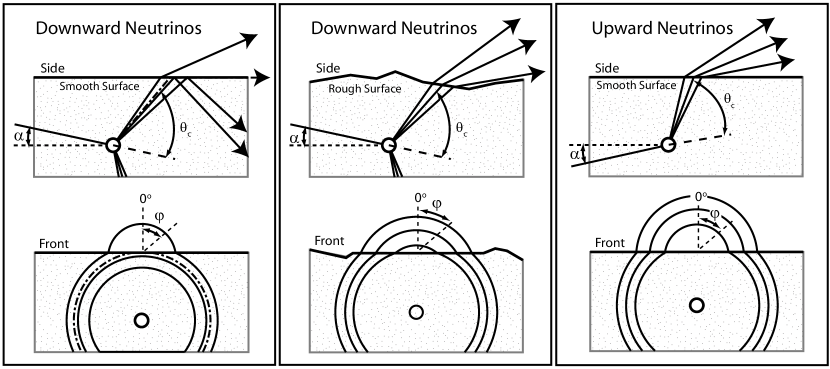
Figure 1: (Left panel) Side and face-on views of Cerenkov cone ray paths escaping the lunar surface for downward-directed neutrinos, assuming a smooth surface. (Middle) Same, but including surface roughness. Note that a larger fraction of the Cerenkov cone escapes. (Right) Same, but for upward-going neutrinos.

Accounting for surface roughness may be accomplished by using a probabilistically smoothed ${\mathcal{H}}_{R}$ function defined by

$${\mathcal{H}}_{R}\ =\ \pi^{-3/2}\int_{-\pi/2}^{\pi/2}d\phi^{\prime}\ \int_{-\infty}^{\infty}dw\ e^{-w^{2}}{\mathcal{H}}_{w,\phi^{\prime}}{{({\hat{n}}_{\sigma}\cdot{\hat{\gamma}})}\over{({\hat{n}}\cdot{\hat{\gamma}})}}\ \cong\ 2\pi^{-3/2}\int_{0}^{\pi/2}d\phi^{\prime}\ \int_{-\infty}^{\infty}dw\ e^{-w^{2}}{{\mathcal{H}}}_{w,\phi^{\prime}}\ ,$$ (4)

which allows the surface normal to be tilted, relative to the radio ray incident along ${\hat{\gamma}}$, by a small polar angle $\sigma=\sigma_{o}w$ in a random azimuthal ($\phi^{\prime}$) direction. The polar angle $\sigma$ is approximately normally distributed with Gaussian halfwidth $\sigma_{o}$, as supported by the findings of Shepard et al. (1995) in the limit of small $\sigma$. The expression $({\hat{n}}_{\sigma}\cdot{\hat{\gamma}})/({\hat{n}}\cdot{\hat{\gamma}})$ accounts for the higher likelihood of encountering a tilt that reduces the angle of incidence than one that increases it, owing to the relative increase in projected area of the former, but this effect is deemed to be too negligible to track when the tilt angles are small, consistent with our other approximations. Here ${{\mathcal{H}}}_{w,\phi^{\prime}}$ expresses the no-internal-reflection selection rule in the form of a step function whose argument is positive whenever the values of $w$ and $\phi^{\prime}$ allow the ray to cross the surface, so ${\mathcal{H}}_{R}$ itself becomes a smoothed function rather than a formal Heaviside function.

It should be noted that we choose the somewhat nonstandard convention of allowing $w$ to be either positive or negative, corresponding to surface tilts that either help or hinder ray escape, and take the azimuth of the surface normal to wrap only from $-\pi/2$ to $\pi/2$ (further applying the left/right symmetry to restrict to one azimuthal quadrant from $0$ to $\pi/2$), rather than restricting the tilt angle to positive values and wrapping around the full $2\pi$ in azimuth. We choose this convention because it indicates more explicitly when the tilt is helping or hindering escape, an issue to which the Heaviside functions are highly sensitive. Also note that ${{\mathcal{H}}}_{R}$ is normalized to unity in the purely hypothetical situation where ${{\mathcal{H}}}_{w,\phi^{\prime}}$ is always unity, as desired.

Including surface roughness can increase the aperture significantly, but it also adds two additional dimensions to the integral over fractional phase space, and it introduces a new angular scale, $\sigma_{o}$, to the several other important angular scales that appear in the calculation. It is natural to expect this complication to be worthwhile whenever $\sigma_{o}$ is appreciable relative to the other angular widths that affect the aperture, for example when observing at high frequencies where the Cerenkov cone is thin. The scaling laws we derive bear out this expectation.

2.3 Isotropic neutrino flux

As the current interest is primarily in cosmologically distributed sources, rather than targeted sources, we focus on isotropic neutrino flux distributions $I(E)$, and simplify the form of the aperture. Then we may write the detection rate ${\mathcal{R}}$ as

$${\mathcal{R}}\ =\ \int dE\ I(E)A(E)\ ,$$ (5)

where the energy-dependent isotropic aperture is given by

$$A(E)={A_{max}}\int d{{\hat{V}}_{m}}\int d{{\hat{\Omega}}_{\gamma}}\int d{{\hat{\Omega}}_{\nu}}\ e^{-\tau_{\nu}}\ {{\mathcal{H}}_{R}}\ {{\mathcal{H}}_{D}}\ .$$ (6)

Again note that each fractional phase space integral is by definition normalized to unity, and ${A_{max}}$ specifies the units of $A(E)$, but not the scale of $A(E)$. The great majority of the fractional phase space will generally not contribute to neutrino detections, and thus $e^{-\tau_{\nu}}$, ${{\mathcal{H}}_{R}}$, and ${{\mathcal{H}}_{D}}$ exert stringent constraints on $A(E)$ in ways we will now calculate.

2.4 Spherical symmetry simplifications

The fractional phase space in eq. (6) includes 7 total dimensions, or 9 including a surface-normal tilt distribution, so would certainly represent a daunting undertaking to compute in closed form. However, we receive welcome assistance from the basic spherical symmetry of the Moon, in concert with an isotropic incident neutrino flux. Capitalizing on that symmetry actually allows us to eliminate three of the dimensions of the phase space (two because the lunar aperture operates the same way as seen by observers from all directions, and one because the lunar aperture seen by those observers has an axial symmetry around the Moon center). This reduces the phase space (even with surface roughness) to 6 dimensions, which is certainly more tractable, though still requiring extensive use of approximations to achieve a closed-form result.

2.5 Aperture calculation from the lunar volume-centered perspective

Several choices are possible for coordinatizing the phase space, each with its various computational advantages and challenges. We adopt a Moon-centered perspective that scans in spherical coordinates over the volume of the Moon by accounting only for the distance $h$ below the lunar surface along the radial direction, and we coordinatize the incident neutrino direction in terms of the glancing angle $\alpha$ that the neutrinos make to the surface (so $\alpha$ is the complement of the angle of incidence to the normal), so chosen because it tends to be a small quantity. Our convention is $\alpha>0$ for upward neutrinos that must penetrate a significant lunar secant before reaching the detectable zone.

Hence, the 4-dimensional configuration phase space is divided into one dimension to describe the location of interest in the Moon, one dimension to describe the incident neutrino angle, and two dimensions to describe the outgoing electric field rays. At this point in the calculation, we temporarily consider the two dimensions of outgoing radio rays to be outside the Moon, but shortly we will convert to a coordinatization where these are inside the Moon and along the Cerenkov cone of the shower. As mentioned above, in addition to these four dimensions, there are generally two more integrations to account for the local surface normal variations on the scale of the assumed surface roughness.

The crucial simplification stemming from the spherical symmetry and the isotropic neutrino assumption is that fractional phase-space component weights are based only on the probability that a hypothetical observer at Earth distance randomly chosen over the solid angle of the lunar sky could detect the radio signal, without specifying any particular viewing angle. This succeeds because we are in effect fixing the location where the shower occurs along an arbitrary radial ray in the Moon, randomizing the orientation of the observer, and asking what is the probability that such a randomly located observer could detect that shower.

Translating the above into an expression for the aperture yields

$$A(E)\ =\ {A_{max}}(E)\times{1\over 2}\int_{-\pi/2}^{\pi/2}d\alpha\ \cos\alpha\ \times\ \int d{{\hat{\Omega}}_{\gamma}}\ \times\ {3\over R_{m}^{3}}\int_{0}^{R}dr\ r^{2}\ e^{-\tau_{\nu}}{\mathcal{H}}_{D}\ {\mathcal{H}}_{R}\ ,$$ (7)

where $R_{m}$ is the radius of the Moon. Note how each fractional phase space component is still normalized to unity, in keeping with the partition of ${A_{max}}$ over its contributing fractional phase space. Defining the neutrino interaction length to be ${L_{\nu}}(E)=1/\rho\kappa(E)$ for cross section per gram $\kappa(E)$ and mass density $\rho$ (and we take $\rho=1.8$ g cm^-3 in the regolith where the showers occur), we obtain from eq. (1)

$${A_{max}}(E)\ =4\pi M\kappa(E)\ =4\pi\left({4\pi\over 3}R_{m}^{3}\rho\right)\kappa(E)\ =\ {4\over{3}}\ {R_{m}\over{L_{\nu}}}{A_{o}}\ ,$$ (8)

where

$${A_{o}}\ =\ 4\pi^{2}{R_{m}}^{2}$$ (9)

is the maximum attainable aperture for a spherical object for which neutrinos can be detected at most once (see the Appendix for the reason that this “maximum” aperture could actually be exceeded by added contributions from neutrinos with initial energies above $E$). Note that ${A_{o}}$ is the geometric lunar cross section $\pi{R_{m}}^{2}$ times the full 4$\pi$ steradians of illumination, as in Williams (2004), and eq. (7) yields $A(E)={A_{o}}$ if we set ${\mathcal{H}}_{D}{\mathcal{H}}_{R}=1$ and treat $\tau_{\nu}$ in the highly opaque limit, where there is as yet no correction for downgrading of higher-energy neutrinos (again, see the Appendix for how the effective $\tau_{\nu}$ is reduced by downgrading).

Since we treat only neutrino energies for which the Moon is highly opaque, we have ${A_{o}}\ {\ll}\ {A_{max}}(E)$, owing to the high shielding of the lunar interior, and thus ${A_{o}}$ makes for a better fiducial reference to use in our aperture expressions. Thus we will express the aperture $A(E)$ in the form

$$A(E)\ =\ {A_{o}}\ P(E)\ ,$$ (10)

where $P(E)$ is to be interpreted as the fraction of neutrinos entering the Moon at energy $E$ that will actually be detected by the instrument under consideration, assuming all such neutrinos will create showers, and corrected slightly for the detection of downgraded neutrinos originally at higher $E$ (see the Appendix).

2.6 Converting from exterior to interior ray angles

Since detectability of the radio rays is a crucial issue, the field strengths generated by the hadronic showers appear prominently in the aperture calculation. However, the characteristics of these fields trace the Cerenkov cone inside the lunar material, whereas the ray-angle phase space is referenced to the emergent solid angle outside the Moon where the detector is located. This is inconvenient, so we now convert the ray angles to being inside the Moon where the field properties are more easily expressed. To effect that change, we must not only convert $d{{\hat{\Omega}}_{\gamma}}$ to an angular integral over an interior solid angle, we must also account for the solid-angle magnification factor that appears whenever emerging rays refract across a dropping index of refraction, which here falls from its internal value of $n_{r}\cong 1.73$ (James & Protheroe, 2009) to unity. This magnification factor is (e.g., Gorham et al., 2004)

$$\xi(\beta)\ =\ {n_{r}^{2}\cos\beta\over\sqrt{1-n_{r}^{2}\sin^{2}\beta}}\ ,$$ (11)

where $\beta$ is the angle of incidence from the normal of the radio ray as it encounters the lunar surface from the inside.

We coordinatize this interior-ray solid angle using the polar angle $\Delta$ (measured relative to the Cerenkov angle $\theta_{c}$ so the $\Delta$ of interest are usually quite small), and the azimuthal angle $\phi$ around the Cerenkov cone (with the convention that $\phi=0$ corresponds to the direction nearest to the surface). Hence we replace the normalized solid angle $d{{\hat{\Omega}}_{\gamma}}$ by the transformed solid angle $d\Delta\ \sin(\theta_{c}+\Delta)d\phi\ \xi(\beta)/2\pi$, where we take $\phi$ only from 0 to $\pi$ because of the left/right local symmetry. The interior phase space element has its normalization altered by the $\xi(\beta)$ factor, but the resulting exterior solid angle will not exceed its full unit value because the contributing interior solid angle is actually quite small, owing to truncation by ${\mathcal{H}}_{R}$ as seen below.

Indeed we expect all integrals to be truncated by the selection rules imposed by ${\mathcal{H}}_{R}$ and ${\mathcal{H}}_{D}$, so as a minor convenience we will extend all finite integration limits to infinity. This step has no physical significance and will not alter the outcome of the calculation, it merely removes unnecessary emphasis from the arbitrary limits of the integrals, and returns the emphasis to the selection rules themselves. Since we are working in the limit where the radio rays are rapidly attenuated in the Moon, we assume all detections occur near the surface, so we also replace the integral over $r$ with an integral over $z=h/{L_{\gamma}}$, where $h$ is the depth below the surface and ${L_{\gamma}}$ is the electric field dissipation length (so ${L_{\gamma}}/2$ is the photon mean-free-path). We also approximate $r^{2}$ by $R_{m}^{2}$ in the $z$ phase-space integration. These are all excellent approximations in the domain of interest of our calculation.

Taking the definition of $P(E)$ from eq. (10), we combine eqs. (7) and (8) to yield

$$P(E)\ =\ {1\over\pi}\ {{L_{\gamma}}\over{L_{\nu}}}\ \int_{-\infty}^{\infty}d\alpha\ \cos\alpha\ \int_{-\infty}^{\infty}d\Delta\ \sin(\theta_{c}+\Delta)\ \int_{0}^{\infty}d\phi\ \int_{0}^{\infty}dz\ e^{-\tau_{\nu}}\ {\mathcal{H}}_{R}\ {\mathcal{H}}_{D}\ \xi\ .$$ (12)

Note that already the scale of $A(E)$ has been reduced by the factor ${L_{\gamma}}/{L_{\nu}}\ll 1$, the proportion by which neutrinos overpenetrate to depths beyond where detectable electric fields can emerge. The remaining factors that will further reduce the aperture, mediated by the ${\mathcal{H}}$ truncations, will be included next, and will invoke additional approximations.

2.7 Imposing the ${\mathcal{H}}_{R}$ and ${\mathcal{H}}_{D}$ selection rules

The constraint described by ${\mathcal{H}}_{w,\phi^{\prime}}$ is that the radio ray emergent from the electron shower must not internally reflect at the surface of the Moon, and the constraint described by ${\mathcal{H}}_{D}$ is that the signal be detectable by the instrument of interest. Each Heaviside function uses whichever quantity must be positive to apply the constraint, which appropriately truncates the limits of integration.

We first consider the requirement that we count the contribution only from rays that are associated with detectably strong radio waves. We assume that each shower induces a Cerenkov cone with a field strength along each ray that depends on the deviation $\Delta$ in polar angle from the Cerenkov peak angle $\theta_{c}$. If the field strength ${\mathcal{E}}$ is distributed over $\Delta$ in an approximately Gaussian way (small deviations from this are discussed by Scholten et al., 2006; Gusev et al., 2006), then

$${\mathcal{E}}\ =\ {\mathcal{E}}_{o}{\hat{t}_{\parallel}}(\beta)\ e^{-(\Delta/\Delta_{o})^{2}}\ e^{-\tau_{\gamma}}\ ,$$ (13)

where $\Delta_{o}$ is the Gaussian halfwidth of the angular distribution around the Cerenkov angle, ${\mathcal{E}}_{o}$ is the strength of the field at the shower along the Cerenkov angle, $\tau_{\gamma}$ is the number of radio dissipation lengths the field passes through before exiting the Moon at the frequency in question, and ${\hat{t}_{\parallel}}(\beta)$ is the field transmission coefficient appropriate for the diverging rays that fill the emergent solid angle of interest. We assume the polarization is in the plane of incidence (termed “pokey” electric polarization), as that is the dominant polarization for the rays most likely to escape total internal reflection, and $\beta$ is the angle of incidence to the surface normal (inside the Moon).

The result begins with the standard expression for the field transmission coefficient for plane waves (Williams, 2004)

$$t_{\parallel}\ =\ \sqrt{{n_{r}\cos\beta\over\cos\beta_{o}}\ \left(1\ -\ r_{\parallel}^{2}\right)}$$ (14)

where $r_{\parallel}$ is the field reflection coefficient for “pokey” electric polarization, and $\beta_{o}$ is the angle of refraction relative to the normal (outside the Moon) as the rays pass through the surface of the Moon into free space, so

$$\beta_{o}\ =\ \sin^{-1}(n_{r}\sin\beta)\ .$$ (15)

In an appendix of Williams (2004), a ray-tracing technique is described for converting this plane-wave transmission coefficient to one appropriate for the diverging rays that fill the observable emergent solid angle, which agrees with an analytic result she quotes from a private communication with Dave Seckel. The result is

$${\hat{t}_{\parallel}}\ =\ \sqrt{{\tan\beta\over\tan\beta_{o}}\left(1\ -\ r_{\parallel}^{2}\right)}\ =\ {\tan\beta\over\tan\beta_{o}}t_{\parallel}(\beta)\ =\ {2\sin\beta\cos\beta_{o}\over\sin(\beta_{+}\beta_{o})\cos(\beta-\beta_{o})}\ ,$$ (16)

where

$$t_{\parallel}(\beta)\ =\ {2\sin\beta_{o}\cos\beta\over\sin(\beta_{o}+\beta)\cos(\beta_{o}-\beta)}\ .$$ (17)

It may be noted that the Williams (2004) numerical result, the above analytic expression, and the analytic expression cited in Gusev et al. (2006), present sequentially more pessimistic transmission coefficients, at roughly the 10% level per step in the sequence. This motivates both our using the “intermediate” level of optimism, and the application of the rather crude approximation outlined below. It appears that the transmission of diverging radio rays from a hadronic shower remains a problem that is not completely solved.

In this paper we use expressions for the maximum electric field and the Cerenkov cone width in the regolith as given by James & Protheroe (2009), which tend to give narrower detection windows and lower apertures than previous values in the literature. For the maximum field we have

$${\mathcal{E}}_{o}(d,\nu,E)=0.0845\ \frac{\rm{V}}{\rm{m}\cdot\rm{MHz}}\ \left[\frac{d}{m}\right]^{-1}\ \left[\frac{E_{s}}{EeV}\right]\ \left[\frac{\nu}{\rm{GHz}}\right]\ {\left[1+\left(\frac{\nu}{\rm{2.32~{}GHz}}\right)\right]}^{-1.23}\ ,$$ (18)

where $d$ is the distance from the shower (and $m$ is the unit in meters), $\nu$ is the observing frequency, and $E_{s}$ is the shower energy in EeV ($10^{18}$ eV). Approximately 20% of the incident neutrino energy is deposited in hadronic showers, independent of neutrino flavor (James & Protheroe, 2009), so we take $E_{s}=0.2E$. The Cerenkov cone $1/e$ half-width is given by

$$\Delta_{o}=0.05\ \left[\frac{\rm{GHz}}{\nu}\right]\ {\left[1+0.075\ {\rm log}\left(\frac{E_{s}}{10^{19}\rm{eV}}\right)\right]}^{-1}\ .$$ (19)

Note that we have multiplied the angular width constant $C_{H}=2.4\arcdeg$ of (James & Protheroe, 2009) by the factor $1/\sqrt{ln\ 2}=1.2$ to make $\Delta_{o}$ be the $1/e$ half-width rather than the half-width at half-maximum, as this is more attuned to use with the familiar exponential attenuation factors. We also convert the angle units to radians for use in the scaling laws that follow, since radians are the useful unit for testing the small-angle approximations that will be invoked shortly.

For a telescope with a field detection threshold ${\mathcal{E}}_{min}$, the selection rule to have a detectable signal in eq. (13) is

$${\mathcal{E}}_{min}\ <\ {\mathcal{E}}_{o}{\hat{t}_{\parallel}}(\beta)e^{-(\Delta/\Delta_{o})^{2}}\ e^{-\tau_{\gamma}}\ ,$$ (20)

or, solving for $\Delta$,

$$\Delta\ <\ \Delta_{o}\sqrt{{\rm ln}\left({{\hat{t}_{\parallel}}(\beta){\mathcal{E}}_{o}\over{\mathcal{E}}_{min}}\right)\ -\ {s\over{L_{\gamma}}}}\ ,$$ (21)

where $s$ is the path length from the shower to the surface and ${L_{\gamma}}$ is the electric field dissipation length. Therefore ${{\mathcal{H}}}_{D}=0$ when this is not satisfied, which truncates the integrals over $\Delta$ and $z$ in a manner that depends on the order of integration. When the above expression is satisfied, the ray in question is detectable, and ${{\mathcal{H}}}_{D}=1$.

To avoid internal reflection, the ray must meet the surface at an angle of incidence that exceeds the complement of the Cerenkov angle, where the Cerenkov angle is $\theta_{c}=\cos^{-1}(1/n_{r})=0.954$ for $n_{r}=1.73$. The transmission coefficient ${\hat{t}_{\parallel}}(\beta)$ goes to zero at that angle, which is when $\beta=\pi/2-\theta_{c}$, and remains zero for all larger $\beta$. Thus, the constraint in eq. (21) is already violated when internal reflection occurs, and there would be no formal need to include ${\mathcal{H}}_{w,\phi^{\prime}}$ separately. However, ${\hat{t}_{\parallel}}$ grows so rapidly with angle that it is appreciably nonzero even just a few degrees from critical, and it quickly saturates near 0.7 for angles as small as 10 degrees from critical. That rapidly saturating behavior, along with the fact that ${\hat{t}_{\parallel}}$ appears in a logarithm so is only crucially important for weaker fields, motivates our choosing to model ${\hat{t}_{\parallel}}\cong 0.6$ as a constant. This loses some accuracy in the result, but is much computationally simpler than following a function whose small-angle approximation breaks down completely for angles more than just 2 degrees from critical. Uniformly setting ${\hat{t}_{\parallel}}=0.6$ implies that we no longer have zero transmission at the critical angle, so we now need to apply the total internal reflection constraint, ${\mathcal{H}}_{w,\phi^{\prime}}$, separately.

To determine if internal reflection is avoided, we need the cosine of the angle of incidence, which is given by the dot product of the surface normal $\hat{n}(w,\phi^{\prime})$ and the ray direction $\hat{\gamma}(\Delta,\phi,\alpha)$. Here $\alpha$ is the angle the neutrino (and its shower) makes to the horizontal, where our convention is that $\alpha<0$ is for downward neutrinos that are first encountering the Moon close to the shower of interest. Thus given the glancing incident neutrino angle $\alpha$, which sets the orientation of the Cerenkov cone, and the electric field ray angles $\Delta$ and $\phi$ within that cone (where $\Delta=0$ is at the Cerenkov angle and $\phi=0$ is most directly toward the surface and least apt to internally reflect), we require

$$\hat{n}(w,\phi^{\prime})\cdot\hat{\gamma}(\Delta,\phi,\alpha)\ >\ \sin\theta_{c}\ ,$$ (22)

which yields directly

$$\sin\theta_{c}\ <\sin(\theta_{c}+\Delta)\cos\phi\sin\sigma\cos\phi^{\prime}\sin\alpha\ -\ \cos(\theta_{c}+\Delta)\cos\sigma\sin\alpha\\ \ -\ \sin(\theta_{c}+\Delta)\sin\phi\sin\sigma\sin\phi^{\prime}\ +\ \sin(\theta_{c}+\Delta)\cos\phi\cos\sigma\cos\alpha\\ \ +\ \cos(\theta_{c}+\Delta)\sin\sigma\cos\phi^{\prime}\cos\alpha\ .$$ (23)

Applied to the integrals in eq. (12), this constraint identifies a maximum azimuth $\phi$ and truncates the $\phi$ integral there, while the constraint in eq. (21) truncates the integral over depth $z$.

3 Further approximations to reach a result in closed form

The goal of this paper is to achieve closed-form expressions for the effective area $A(E)$ as a function of neutrino energy, lunar regolith properties, and observing parameters. Since at this point we still have a cumbersome 6-dimensional integral to evaluate, we must avail ourselves of several additional approximations to obtain a tractable expression which yields the desired scaling laws.

3.1 The near-surface emission approximation

Since the integrand $e^{-\tau_{\nu}}$ depends on $z$, the $z$ integration is nontrivial, but this dependence is removed when the observable showers have to be so close to the surface that there is no appreciable change in the neutrino irradiation over the region where the radio signals are detectable. The requirement to make this approximation is

$${L_{\gamma}}\ {\ll}\ {{L_{\nu}}^{2}\over R_{m}}$$ (24)

where ${L_{\gamma}}$ and ${L_{\nu}}$ are the electric-field attentuation length and neutrino mean-free-path respectively. This “near-surface emission” approximation allows the $z$-integral to be performed trivially. The expressions for ${L_{\nu}}$ and ${L_{\gamma}}$ are taken as (summing the cross sections for neutral and charged-current interactions, as they both generate similar hadronic showers, Gandhi et al., 1998; Reno, 2005),

$${{L_{\nu}}\over R_{m}}\ =\ 0.07\left({E\over 10^{20}eV}\right)^{-1/3}\left(\rho\over{\rho_{reg}}\right)^{-1}\ ,$$ (25)

where $\rho_{reg}=1.8$ g cm^-3 is the regolith mass density, and

$${{L_{\gamma}}\over R_{m}}\ =\ 1\times 10^{-5}\left({\nu\over GHz}\right)^{-1}\ .$$ (26)

(This result is known only to within about a factor of two (Gorham et al., 2004; Scholten et al., 2006). Hence the approximation requires $\nu\ {\gg}\ 5(E/10^{20}$ eV$)^{2/3}$ MHz for lunar rock with density $\rho\cong 3$ g cm^-3. This is satisfied over most of the range of neutrino energies and radio frequencies that concern us, except when the lowest frequencies ($\nu\mathrel{\hbox to0.0pt{\lower 3.0pt\hbox{$\mathchar 536\relax$}\hss}\raise 2.0pt\hbox{$\mathchar 316\relax$}}100$ MHz) are used to observe the highest energy ($E{\gg}10^{22}$ eV) neutrinos.

The surface-emission approximation allows us to replace $\tau_{\nu}$ in $e^{-\tau_{\nu}}$ by

$$\tau_{\nu}\ \cong\ {R_{m}\over\psi{L_{\nu}}}\sin\alpha\ {\mathcal{H}}(\alpha)$$ (27)

for ${\mathcal{H}}(\alpha)$ again the Heaviside step function, so $\tau_{\nu}=0$ for $\alpha<0$ (downward neutrinos) and $\tau_{\nu}\ =\ \sin\alpha\times 2R_{m}/{L_{\nu}}$ for $\alpha>0$ (upward neutrinos). Here we insert the order-unity parameter $\psi=1.4$ (appropriate for a neutrino spectrum $\sim E^{-2}$, see Appendix) to account for neutrinos from higher energies being downgraded into the detection regime for energy $E$, which slightly enhances the aperture. Note the absence of dependence on $z$, making the $z$ integration a trivial matter of simply tracking its range of contribution.

Carrying out the $z$ integration subject to the selection rule in equation (21) and using

$${s\over{L_{\gamma}}}\ =\ {z\over\sin(\theta_{c}+\Delta)\cos\phi\cos\alpha\ -\ \cos(\theta_{c}+\Delta)\sin\alpha}\ ,$$ (28)

the detection probability integral (eq. [12]) can be written

$$P(E)\ =\ {2\over\pi^{5/2}}\ {{L_{\gamma}}\over{L_{\nu}}}\ \int_{-\infty}^{\infty}d\alpha\ \cos\alpha\ \int_{-\infty}^{\infty}d\Delta\ \sin(\theta_{c}+\Delta)\ \\ \times\int_{0}^{\infty}d\phi\ \int_{0}^{\pi/2}d\phi^{\prime}\ \int_{-\infty}^{\infty}dwe^{-w^{2}}\Upsilon(z_{max})\ e^{-\tau_{\nu}}\ {\mathcal{H}}_{w,\phi^{\prime}}\ \xi(\beta)\ ,$$ (29)

where $z_{max}$ is the maximum depth for which the emergent field exceeds the minimum detectable value, and we define

$$\Upsilon(f)\ =\ f{\mathcal{H}}(f)$$ (30)

for ${\mathcal{H}}$ the Heaviside step function, to insure the integrand never contributes when it is negative. We may determine $z_{max}$ by combining eqs. (21) and (28)

$$z_{max}\ =\ [\sin(\theta_{c}+\Delta)\cos\phi\cos\alpha\ -\ \cos(\theta_{c}+\Delta)\sin\alpha]\ f_{o}^{2}\left(1\ -\ {\Delta^{2}\over f_{o}^{2}\Delta_{o}^{2}}\right)$$ (31)

where $f_{o}$ is the dimensionless quantity

$$f_{o}\ =\ \sqrt{{\rm ln}\left({{\mathcal{E}}_{o}{\hat{t}_{\parallel}}\over{\mathcal{E}}_{min}}\right)}\ .$$ (32)

Physically, $f_{o}$ is the ratio of the thickness of the Cerenkov cone corresponding to the electric field threshold to the $1/e$ full thickness ($2\Delta_{o}$), as shown in Fig. 2.

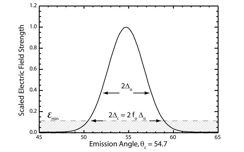
Figure 2: Cerenkov cone angular profile at $E=10^{21}$ eV and $\nu=$ 1 GHz. The dimensionless factor $f_{o}$ is the ratio of the cone thickness at threshold ${\mathcal{E}}_{min}$ to the $1/e$ width.

3.2 Small angle approximation

We have now reduced the number of integrations to five, including two over surface roughness. One more integration, that over azimuthal angle around the Cerenkov cone $\phi$, can be carried out surprisingly easily if we make the further approximation that the detectable radio rays hug tightly to the Cerenkov cone, such that $\Delta$ is small, and that the other angles we treat, $\phi$, $\alpha$, and $\sigma$, are also small. The small-angle approximation is particularly valid for lower energy neutrinos near the important GZK cutoff. It also applies to higher observing frequencies above 1 GHz, and may extend to lower frequencies as long as the highest energy neutrinos are not the focus. In this approximation, the maximum azimuthal angle that does not totally internally reflect, $\phi_{R}$, is given by equation (23) to be

$$\phi_{R}\ =\ \sqrt{{2\left(\Delta\ +\ w\sigma_{o}\cos\phi^{\prime}\ -\ \alpha\right)\over\tan\theta_{c}}}\ \ ,$$ (33)

which supplies the upper limit for the $\phi$ integration.

The small-angle approximation also permits us to use

$$z_{max}\ \cong\ \sin\theta_{c}\ f_{o}^{2}\left(1\ -\ {\Delta^{2}\over f_{o}^{2}\Delta_{o}^{2}}\right)\ ,$$ (34)

and to replace $\sin\theta$ by $\sin\theta_{c}\ =\ \sqrt{1-1/n_{r}^{2}}$ and $\cos\alpha$ by unity. This gives us all the expressions we need to simplify the evaluation of the integrals, recalling again that $f_{o}$ is influenced by ${\hat{t}_{\parallel}}$, and to within an expected accuracy of 10-20% we take ${\hat{t}_{\parallel}}(\beta)=0.6$, rather than its small-angle form, as the latter loses accuracy too rapidly for the angles we need to treat. We note that the primary influence of ${\hat{t}_{\parallel}}$ is in determining the depth below the surface that will be visible, and since the angular contributions scale in a self-similar way as this depth is varied at different $E$, the systematic errors introduced by our approach should appear primarily in the energy scale. Hence the transmission coefficient has its largest significance in the determination of the minimum detectable neutrino energy, and since this is already an important issue for GZK-type neutrinos, future work should attempt to clarify the reliability of the various and somewhat contradictory treatments of ${\hat{t}_{\parallel}}$ found in the literature.

3.3 Evaluation of the azimuthal integral over the Cerenkov cone

Approximating all remaining angles to lowest nonvanishing order simplifies the expressions dramatically, and allows us to carry out the $\phi$ and $w$ integrations in closed form. Prior to those integrations, and subject to the approximations above, the detection probability becomes

$$P(E)\ ={2\over\pi^{5/2}}{(n_{r}^{2}-1)\over n_{r}^{2}}f_{o}^{2}\left({{L_{\gamma}}\over{L_{\nu}}}\right)\int_{-\infty}^{\infty}dw\ e^{-w^{2}}\int_{0}^{\pi/2}d\phi^{\prime}\ \\ \times\int_{-\infty}^{\infty}d\Delta\ \Upsilon\left(1\ -\ {\Delta^{2}\over f_{o}^{2}\Delta_{o}^{2}}\right)\int_{-\infty}^{\infty}d\alpha\ e^{-\tau_{\nu}}\int_{0}^{\phi_{R}}d\phi\ \xi(\beta){\mathcal{H}}_{R}(\phi_{R})\ ,$$ (35)

where in the surface-emission approximation we have

$$\tau_{\nu}\ =\ \Upsilon\left({\alpha\over\alpha_{o}}\right)$$ (36)

and we have defined

$$\alpha_{o}\ =\ {{L_{\nu}}\psi\over 2R_{m}}\ =\ 0.03\left({E\over 10^{20}eV}\right)^{-1/3}$$ (37)

as the angle through which upward ($\alpha>0$) neutrinos are successful at penetrating the lunar secant through rock with mass density $\rho=$ 3 g cm^-3 up to the regolith layer (with $\psi\cong 1.4$ chosen in regard to a somewhat arbitrary neutrino spectrum with power-law index -2, see Appendix).

To evaluate the $\phi$ integral, let us first let us define the angle $\varepsilon$, which is the angle of incidence (from inside the Moon) to the normal to the surface, relative to the critical angle, so

$$\varepsilon\ =\ {\pi\over 2}\ -\ \theta_{c}\ -\ \beta\ .$$ (38)

We replace $\beta$ by $\varepsilon$ because the latter is small and will be considered only to lowest nonvanishing order. To this order, we find eq. (11) becomes

$$\xi(\varepsilon)\ \cong\ {n_{r}(n_{r}^{2}-1)^{1/4}\over\sqrt{2\varepsilon}}\ ,$$ (39)

which demonstrates explicitly how the solid-angle magnification factor gets large as the critical angle is approached. This magnification effect is an important contributor to what would otherwise be a much smaller aperture.

The angle $\varepsilon$ is not one of the phase space integration variables, but is easily expressed in terms of those variables, in the small-angle limit:

$$\varepsilon\ \cong\ \Delta\ +\ w\sigma_{o}\cos\phi^{\prime}\ -\ \alpha\ -\ {\sqrt{n_{r}^{2}-1}\over 2}\phi^{2}\ =\ {\sqrt{n_{r}^{2}-1}\over 2}\phi_{R}^{2}\left(1\ -\ {\phi^{2}\over\phi_{R}^{2}}\right)\ ,$$ (40)

where in this limit we have

$$\phi_{R}\ =\ {2(\Delta+w\sigma_{o}\cos\phi^{\prime}-\alpha)\over\sqrt{n_{r}^{2}-1}}\ .$$ (41)

Now we encounter an interesting result, which follows from elementary application of eqs. (39) and (40):

$$\int_{0}^{\phi_{R}}d\phi\ \xi(\varepsilon){\mathcal{H}}(\phi_{R})\ =\ {n_{r}\pi\over 2}{\mathcal{H}}(\phi_{R})$$ (42)

for any set of values for the other phase-space variables. In other words, in each equal-size phase-space bin over $\Delta$, $\alpha$, $\sigma$, and $\phi^{\prime}$, the integral over $\phi$ yields either the same fixed numerical value, or it vanishes. Physically, this says that the solid-angle magnification effect perfectly compensates for the way internal reflection truncates the azimuthal window for ray escape. This can be no coincidence, and presumably would be more intuitively clear using some other choice of phase-space partition.

3.4 Evaluation of the integral over incident neutrino angle

The simple result from the $\phi$ integration is especially helpful in carrying out the integral over $\alpha$, because it adds no new dependence on $\alpha$ to the integrand. Thus the integrand remains simply $e^{-\Upsilon(\alpha/\alpha_{o})}$, which is amenable to closed-form integration. When $\alpha>0$ (upward neutrinos), we have an exponential integral, and when $\alpha<0$ (downward neutrinos), we have a trivial integrand.

At this point it is convenient to introduce the scaled variables

$$v\ =\ {\alpha\over\alpha_{o}}$$ (43)

and

$$u\ =\ {\Delta\over f_{o}\Delta_{o}}\ ,$$ (44)

and define the “roughness parameter”

$$x\ =\ {\sigma_{o}\over f_{o}\Delta_{o}}\ ,$$ (45)

which characterizes how the window of acceptance of downward neutrinos can be expanded by surface tilts that avoid total internal reflection, and the “penetration parameter”

$$y\ =\ {\alpha_{o}\over f_{o}\Delta_{o}}\ ,$$ (46)

which characterizes the contribution of upward neutrinos that penetrate a long distance through the lunar rock to reach the shower point. Using these definitions, eq. (35) becomes

$$P(E)\ =\ P_{o}(E)\alpha_{o}\int_{0}^{\pi/2}d\phi^{\prime}\ \int_{-\infty}^{\infty}dw\ e^{-w^{2}}\int_{-1}^{1}du\ (1-u^{2})\int_{-\infty}^{\infty}dv\ e^{-\Upsilon(v)}{\mathcal{H}}(v-v_{min})$$ (47)

where for brevity we define

$$P_{o}(E)\ =\ {(n_{r}^{2}-1)\over\pi^{3/2}n_{r}}\left({{L_{\gamma}}\over{L_{\nu}}}\right)f_{o}^{3}\Delta_{o}$$ (48)

and

$$v_{min}\ =\ -{u\over y}\ -\ {wx\cos\phi^{\prime}\over y}\ .$$ (49)

The integration over $v$ may be carried out explicitly, yielding

$$P(E)\ =\ P_{o}(E)\ \alpha_{o}\int_{0}^{\pi/2}d\phi^{\prime}\ \\ \times\left[\int_{w_{o}}^{\infty}\ e^{-w^{2}}\int_{-1}^{1}du\ (1-u^{2})U_{+}\ +\ \int_{-w_{o}}^{w_{o}}dw\ e^{-w^{2}}\int_{w/w_{o}}^{1}du\ (1-u^{2})U_{-}\right]$$ (50)

where $w_{o}\ =\ 1/(x\cos\phi^{\prime})$ and

$$U_{\pm}\ =\ 1\ +\ {u\over y}\ \pm\ {wx\cos\phi^{\prime}\over y}\ +\ e^{\pm(u/y\ -\ wx\cos\phi^{\prime}/w_{o})}\ .$$ (51)

Although further progress can be made carrying out the elementary integrals over the Cerenkov cone angle $u$, the expressions become extremely unwieldy, and the two further integrals over the surface tilt parameters $w$ and $\phi^{\prime}$ would require numerical integration anyway. So we pursue no further the formal integration of these expressions, and instead turn to calculating scaling laws in various asymptotic limits. We ultimately find that a convenient global approximation may be derived without significant loss of accuracy, by using the approximate method described next.

3.5 Asymptotics and scaling laws

Since the ultimate goal is to gain insight by deriving scaling laws and asymptotic limits, we seek an approximate evaluation of eq. (50) that is accurate in both limits of weak and strong roughness ($x\rightarrow 0$ and $x\ {\gg}\ 1$, respectively), which will then hopefully maintain approximate accuracy in between. We may accomplish this simply by evaluating the aperture in these two opposite extremes, keeping only the leading contributions in each regime, and simply adding them together for a global scaling law. Because the regimes of contribution are so physically separable, simply adding them produces results that agree with the full expressions within $\sim$25%, and also yields physically insightful results.

Taking $x=0$ produces closed-form results for the integral in eq. (50), but even those results are more complicated than necessary. Keeping only the dominant terms in the limit of either large or small $y$, we find we achieve better than 25% accuracy with the simple asymptotic expression

$$P(E)_{smooth}\ \cong\ {(n_{r}^{2}-1)\over 8n_{r}}{{L_{\gamma}}\over{L_{\nu}}}f_{o}^{3}\Delta_{o}\left(f_{o}\Delta_{o}\ +\ {16\over 3}\alpha_{o}\right)\ .$$ (52)

Note the first term in the parentheses originates from downward neutrinos and the second from upward neutrinos, so we see the angular acceptance of downward neutrinos is controlled by the Cerenkov width when the surface is smooth, and the acceptance of upward neutrinos is due to the angle that can successfully penetrate the Moon.

If we include roughness and consider the limit $x\ {\gg}\ 1$, we find that the upward neutrino detection rate is hardly affected, because upward detections are limited far moreso by penetration than by total internal reflection, giving them a completely different character from downward detections. However, the downward detection rate may be greatly enhanced by roughness, because downward neutrinos often produce Cerenkov cones that are almost completely internally reflected unless the surface encountered by the rays is favorably tilted, and we find in this limit

$$P(E)_{rough}\ \cong\ {(n_{r}^{2}-1)\over 8n_{r}}{{L_{\gamma}}\over{L_{\nu}}}f_{o}^{3}\Delta_{o}\left({16\over 3\pi^{3/2}}\sigma_{o}\right)\ ,$$ (53)

so the role of $f_{o}\Delta_{o}$ for the downward neutrinos has been supplanted by $\sigma_{o}$; rays avoid internal reflection not by pushing to the edge of the detectable Cerenkov cone, but rather by being lucky enough to encounter the surface where the tilt is highly favorable.

Adding the smooth and rough limits thus yields the general expression, consistent with pre-existing inaccuracies owing to the idealizations and approximations already in place. Thus we find for the full aperture calculation

$$A(E)\ \cong\ A_{o}{(n_{r}^{2}-1)\over 8n_{r}}{{L_{\gamma}}\over{L_{\nu}}}f_{o}^{3}\Delta_{o}\left(\Psi_{ds}\ +\ \Psi_{dr}\ +\ \Psi_{u}\right)\ ,$$ (54)

where

$$\Psi_{ds}\ =\ f_{o}\Delta_{o}$$ (55)

accounts for downward detections without help from roughness,

$$\Psi_{dr}\ =\ {16\over 3\pi^{3/2}}\sigma_{o}\ =\ 0.96\ \sigma_{o}$$ (56)

accounts for downward detections assisted by roughness, and

$$\Psi_{u}\ =\ {16\over 3}\alpha_{o}\ =\ 5.3\ \alpha_{o}$$ (57)

accounts for the detection of upward neutrinos.

The above results underline clearly the three basic angular scales of interest, the Cerenkov width $\Delta_{c}=f_{o}\Delta_{o}$, the surface roughness parameter $\sigma_{o}$, and the upward neutrino acceptance angle $\alpha_{o}$, which with appropriate coefficients, map into the angular acceptance parameters $\Psi_{ds}$, $\Psi_{dr}$, and $\Psi_{u}$. The aperture for neutrino detection is simply dominated by whichever of these is largest, and note that the $\alpha_{o}$ angle for upward neutrinos is benefited by an order-unity coefficient that is significantly larger than the others, owing to the much higher azimuthal angular acceptance when internal reflection is less of a problem. Nevertheless, the large scale of $\sigma_{o}$ ($>10\arcdeg$ at $\nu\gtrsim 1$ GHz) makes roughness an important contributor, especially at higher frequencies, whereas the $f_{o}\Delta_{o}$ parameter is largest at low frequencies. Upward neutrinos, on the other hand, prefer lower energy neutrinos that penetrate over a wider $\alpha_{o}$, but are often difficult to detect unless the instrument is extremely sensitive.

4 Aperture Dependence on Lunar and Telescope Parameters

The scaling laws provided by equation (54) may be viewed as the fundamental result of this paper. Each of the three terms has a simple physical interpretation that can be conceptualized in the following simple form:

$$P_{i}\ =\ P_{o}\ \Psi_{i}$$ (58)

for $i={ds,dr,u}$, and where

$$P_{o}\ =\ {(n_{r}^{2}-1)\over 8n_{r}}{{L_{\gamma}}\over{L_{\nu}}}f_{o}^{3}\Delta_{o}$$ (59)

accounts for the inherent angular width of the Cerenkov emission as well as the fractional loss in detections owing to the overpenetration of neutrinos past the layers where radio rays may be detected. The $\Psi_{i}$ terms represent effective acceptance angles for the “active” neutrinos, i.e., the neutrinos that can contribute to detections. The relative contribution of these terms to the total aperture is illustrated in Fig. 3 for a threshold field ${\mathcal{E}}_{min}=0.01$ $\mu$V m^-1MHz^-1 and two characteristic frequencies, 150 MHz and 1.5 GHz.

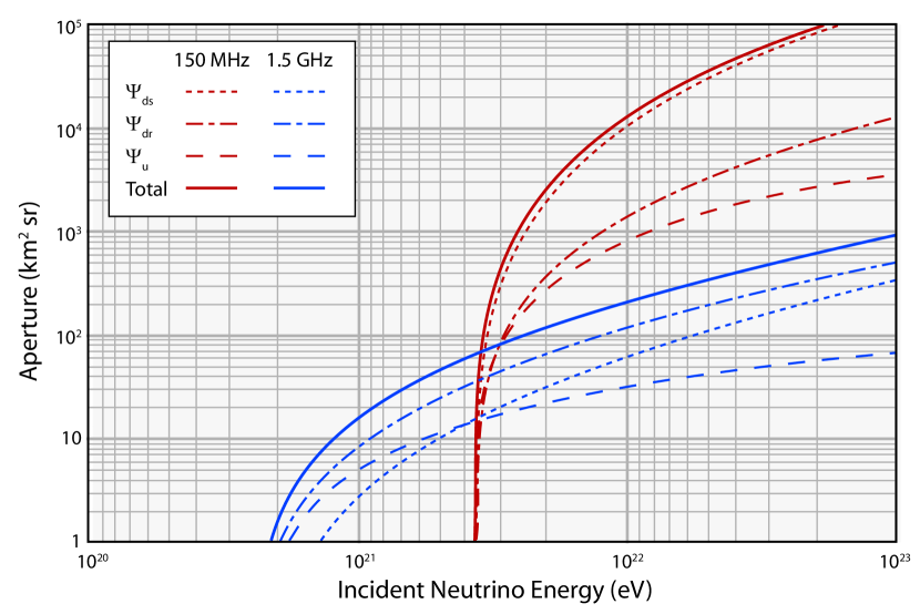
Figure 3: Total aperture versus neutrino energy at threshold field ${\mathcal{E}}_{min}$ = 0.01  $\mu$V m^-1MHz^-1 and two observing frequencies: 150 MHz (solid red line) and 1.5 GHz (solid blue line). The contribution from each of the three terms in equation (54) is also shown. At both frequencies, downward-directed terms have the largest contribution except near the lower cutoff energy. For energies well above the cutoff energy, surface roughness has the largest contribution, except at low frequencies, where the smooth surface term already dominates without assistance from roughness.

4.1 Dependence on Surface roughness

It is apparent from Fig. 3 that the surface roughness contribution $\Psi_{dr}$ is the largest contributor to the total aperture at 1.5 GHz, whereas it is unimportant at 150 MHz. The roughness contribution can be very large at even higher frequencies e.g., the GLUE experiment at 2.2 GHz (Gorham et al., 2004), where the enhancement over a smooth lunar surface is a more than a factor of 3 at $E=10^{21}$ eV. The contribution from surface roughness is important when it exceeds the sum of the contributions from the smooth surface and upward-going contributions For $E_{\nu}=1$ ZeV, this occurs at $\nu\mathrel{\hbox to0.0pt{\lower 3.0pt\hbox{$\mathchar 536\relax$}\hss}\raise 2.0pt\hbox{$\mathchar 318\relax$}}$ 300 MHz with only a modest dependence on neutrino energy. The importance of surface roughness to the detection aperture at high frequencies has also been found in several Monte Carlo ray-tracing simulations of the escaping radiation from the lunar surface (Gorham et al., 2001; Beresnyak, 2003; James & Protheroe, 2009).

4.2 Dependence on minimum detectable electric field (${\mathcal{E}}_{min}$)

The minimum detectable electric field of a radio telescope with effective collecting area $A_{e}$, system temperature $T_{sys}$, and bandwidth $\Delta\nu$, receiving linearly-polarized radiation, can be written (Gorham et al., 2004)

$${\mathcal{E}}_{min}=N_{\sigma}\ {\left(\frac{2k_{b}T_{sys}Z_{0}}{A_{e}\Delta\nu\ n_{r}}\right)}^{\text@frac{1}{2}}\ \ \rm{V/m}$$ (60)

where $N_{\sigma}$ is the minimum number of standard deviations needed to reject statistical noise pulses, $k_{b}$ is Boltzmann’s constant, $Z_{0}$ = 377 $\Omega$ is the impedance of free space, and $n_{r}$ is the refractive index of the medium. This minimum electric field is plotted as a function effective telescope collecting area in Fig. 4, using nominal values of $N_{\sigma}$ = 4.0, $T_{sys}=120\arcdeg$ K (assumed dominated by the Moon’s contribution, limb pointing), and $n_{r}=1.73$.

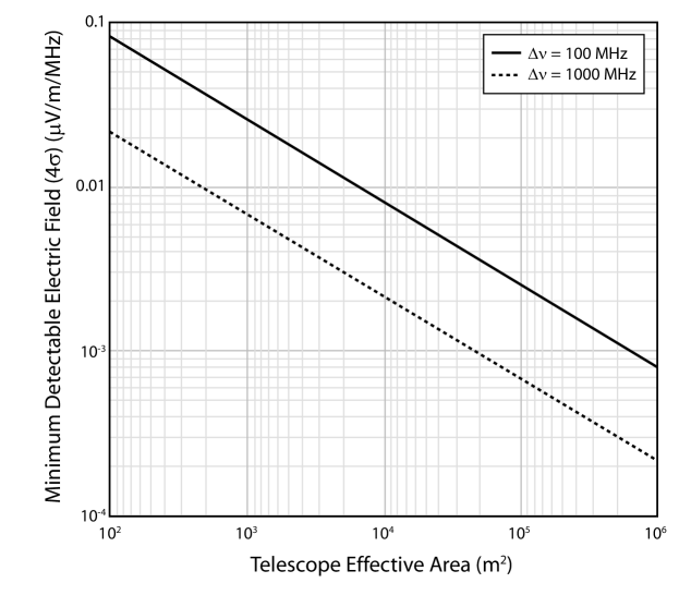
Figure 4: Minimum detectable electric field vs telescope effective area using eq. (60) and bandwidth $\Delta\nu=$100 MHz (solid line) and 1 GHz (dashed line). See text for assumed values for other telescope parameters.

Since the effective thickness of the Cerenkov cone $\Delta_{c}$ depends strongly on ${\mathcal{E}}_{min}$, the total effective aperture will also depend strongly on ${\mathcal{E}}_{min}$, as shown in Fig. 5. The left panel shows the aperture at an observing frequency 1.5 GHz, while the right panel is at 150 MHz. This plot shows the clear trade-off between collecting area and minimum detectable neutrino energy as the observed frequency changes: at high frequencies the minimum neutrino energy cutoff is lower, while at low frequencies the total aperture is significantly higher at a given fixed telescope sensitivity (${\mathcal{E}}_{min}$).

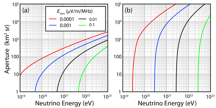
Figure 5: $(a)$ Aperture vs. neutrino energy at observing frequency $\nu=$ 1.5 GHz using telescopes with minimum detectable electric field ${\mathcal{E}}_{min}$= 0.0001, 0.001, 0.01, and 0.1 $\mu$V m^-1MHz^-1 . $(b)$ Same as panel $(a)$, but at observing frequency $\nu=150$ MHz. Note the trade-off between collecting area and minimum detectable neutrino energy as frequency is changed.

The aperture dependence as a function of both telescope sensitivity (${\mathcal{E}}_{min}$) and observing frequency is shown as a surface plot in Fig. 6. Panel (a) shows the total aperture for neutrino energies exceeding $10^{21}$ eV, while panel (b) shows aperture values for $E>10^{22}$ eV. The dark blue regions (zero aperture) correspond to the low-$E$ cutoffs seen in Figs. 3 and 5. Note that for a fixed neutrino energy and telescope sensitivity (${\mathcal{E}}_{min}$), the maximum aperture results from choosing the lowest observing frequency that avoids the sharp cut-off region.

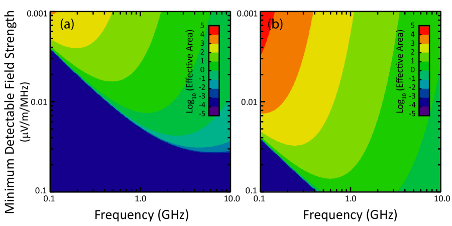
Figure 6: $(a)$ Aperture vs. minimum detectable electric field and observing frequency for neutrinos with energies $E>10^{21}$ eV. $(b)$ Same as panel $(a)$, but for neutrino energies $E>10^{22}$ eV.

4.3 Aperture optimization

One benefit of scaling laws is the ability to make optimization calculations using analytic derivatives. The aperture is energy sensitive, so to maximize the neutrino detection rate, we must make some assumption about the neutrino energy spectrum. We will consider two cases: a power-law distribution and a mono-energetic spectrum.

First consider a canonical power-law neutrino spectrum that scales with neutrino energy as $E^{-2}$. We wish to choose frequency $\nu$ to optimize

$${\mathcal{R}}\ \propto\ \int dE\ E^{-2}P(E)\ .$$ (61)

Let us first assume that the surface roughness dominates the aperture, so we use $\Psi_{dr}$, and note that this will be most appropriate at higher frequencies where the detectable Cerenkov cone is narrow. Then

$${\mathcal{R}}\ \propto\ \int dE\ E^{-2}{{L_{\gamma}}\over{L_{\nu}}}f_{o}^{3}\Delta_{o}\ ,$$ (62)

so

$${\mathcal{R}}\ \propto\ \nu^{-2}\int dE\ E^{-5/3}\left[ln\left({\nu\ E\over 1+(\nu/2.3)^{1.23}}\right)\ +\ k\right]^{3/2}\ .$$ (63)

We can scale the frequency out of the energy integration using $y=\nu E$, and neglecting the weak dependence in the $\nu/2.3$ GHz term in the logarithm, yields that ${\mathcal{R}}$ scales nearly with $\nu^{-4/3}$. Thus the optimal frequency to maximize aperture is as low as possible, at the expense of increasingly larger neutrino cut-off energy sensitivity and technical issues such as RF interference and ionospheric pulse dispersion.

If, on the other hand, if we are targeting a particular energy $E_{o}$, we can focus ${\mathcal{R}}$ on just that $E_{o}$, and find

$${\mathcal{R}}\ \propto\ \nu^{-2}\left[ln\left({\nu\ E\over 1+(\nu/2.3)^{1.23}}\right)\ +\ k\right]^{3/2}\ .$$ (64)

Evaluating the derivative of this expression, again neglecting the variation in the $1+(\nu/2.3)$ term, leads to the conclusion that the detection rate is optimized when the frequency is chosen such that $f_{o}=\sqrt{3/4}=0.87$. This means that for for detection of neutrinos at energy $E_{o}$, $f_{o}$ values substantially above unity are wasting aperture and would be better served by reducing $\nu$ (and $f_{o}$). Likewise, $f_{o}$ values substantially below unity are encountering the energy cutoff problem, so it is preferable to increase the observing frequency.

At low frequencies surface roughness no longer dominates, and instead it is the broadly detectable Cerenkov cones that controls the aperture ($\Psi_{ds}$) for higher energy neutrinos. Then we would find for an $E^{-2}$ power law

$${\mathcal{R}}\ \propto\ \nu^{-3}\int dE\ E^{-5/3}\left[ln\left({\nu\ E\over 1+(\nu/2.3)^{1.23}}\right)\ +\ k\right]^{2}\ ,$$ (65)

which scales roughly like $\nu^{-7/3}$ and favors even more heavily the lower frequencies. However, if a particular energy $E_{o}$ is the target, optimization occurs near $f_{o}=\sqrt{2/3}=0.82$.

In summary, for power-law neutrino spectra with no high-energy cutoff, the detection rate is maximized at the lowest possible observing frequency, neglecting technical problems with RF interference and ionospheric dispersion. However, if a search is optimized for a particular neutrino energy range, the aperture (and consequent event rate) is maximized when the dimensionless parameter $f_{o}\sim 0.8$. From eq. (32) this condition can be written

$$\frac{{\mathcal{E}}_{o}}{{\mathcal{E}}_{min}}=e^{{f_{o}}^{2}}\sim 1.9$$ (66)

We can recast this condition to a more tractable form using eq. (18),

$$\nu_{opt}\ {\left[1+{\left(\frac{\nu_{opt}}{2.32}\right)}^{1.23}\right]}^{-1}=43.2\ \rm{GHz}\cdot{\left[\frac{E}{\rm{ZeV}}\right]}^{-1}\ \left[\frac{{\mathcal{E}}_{min}}{\mu\rm{V\ }\rm{m}^{-1}\rm{\ MHz}^{-1}}\right]\ ,$$ (67)

where $\nu_{opt}$ is the observing frequency which maximizes aperture at neutrino energy $E$.

Fig. 7(a) shows the frequency which maximizes aperture for a given target neutrino energy for threshold sensitivities ${\mathcal{E}}_{min}=$ 0.001, 0.01, and 0.1 $\mu$V m^-1MHz^-1 . Fig. 7(b) plots the aperture as a function of frequency for a threshold sensitivity ${\mathcal{E}}_{min}=$ 0.001 $\mu$V m^-1MHz^-1 for three target energies near the GZK cutoff. As discussed in section 4.2, this sensitivity corresponds to much larger aperture (e.g., SKA) than current searches. Note that the optimal search frequency for GZK neutrinos depends strongly on the exact model for the cosmogenic neutrino energy spectrum, which varies with UHECR source model (e.g., Kalashev et al., 2002).

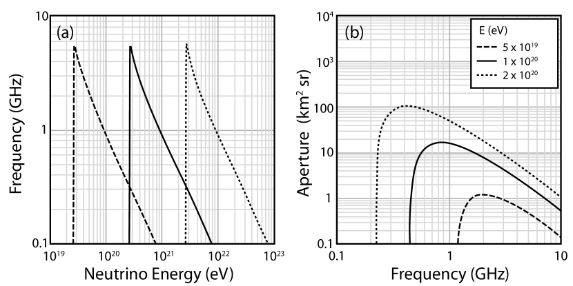
Figure 7: (a) Optimal observing frequency vs. target neutrino energy for threshold ${\mathcal{E}}_{min}$ = 0.001 (dashed line), 0.01 (solid line ), and 0.1 (dotted line) $\mu$V m^-1MHz^-1 . (b) Aperture vs. observing frequency for ${\mathcal{E}}_{min}=0.001$ $\mu$V m^-1MHz^-1 and neutrino energy $E=5\cdot 10^{19}$ eV (dashed line), $\ 10^{20}$ eV (solid line), and $5\cdot 10^{20}$ eV (dotted line).

4.4 Telescope requirements for GZK-neutrino searches

In order to probe near GZK energies ($E\mathrel{\hbox to0.0pt{\lower 3.0pt\hbox{$\mathchar 536\relax$}\hss}\raise 2.0pt\hbox{$\mathchar 316\relax$}}10^{20}$ eV), the minimum detectable electric field must be ${\mathcal{E}}_{min}\mathrel{\hbox to0.0pt{\lower 3.0pt\hbox{$\mathchar 536\relax$}\hss}\raise 2.0pt\hbox{$\mathchar 316\relax$}}10^{-3}$ $\mu$V m^-1MHz^-1 , largely independent of frequency. From Fig. 4 we can see that even for very wide bandwidths, this requires an effective collecting area exceeding 50,000 m², approximately the area of the Arecibo telescope. Since most detection schemes require coincidence on multiple telescopes to discriminate against accidental pulses, an array of multiple Arecibo-class telescopes are required. Current experiments using multiple 10-100 m diameter telescopes can only probe neutrino energies well above GZK, where more exotic neutrino production processes may be operating (e.g., Kalashev et al., 2002). We therefore conclude that only next-generation arrays, e.g., the full SKA ($A_{e}\sim 10^{6}$ m², ${\mathcal{E}}_{min}\sim 10^{-4}$ $\mu$V m^-1MHz^-1 ) will have sufficient collecting area to probe GZK energies. However, even the SKA will have an aperture of only a few km² at the GZK cutoff $E_{GZK}\sim 10^{19.6}$ eV. Given an expected GZK neutrino flux $F_{\nu}\sim$1 km^-1 yr^-1 sr^-1 (e.g., Gusev et al., 2006), the event rate might only be a few counts per observing month. Hence an even higher energy neutrino population, if it exists, might continue to prove easier to detect, even with SKA-class technology.

4.5 Comparison with Monte Carlo simulations

Finally, we address the question of how the present analytic calculations compare with previously published Monte Carlo simulations (e.g., Gorham et al., 2001; Beresnyak, 2003; Williams, 2004; James & Protheroe, 2009). In general, a direct comparison with each simulation is problematic, since the input physics model (neutrino and radio extinction lengths, Cerenkov cone width and peak electric field, lunar roughness, detailed regolith properties) is significantly different for each simulation. However, since we have largely adopted the input physics parameters from James & Protheroe (2009), a direct comparison is warranted in this case.

Table 1 shows a comparison of calculated apertures using the analytic approximation (equation 54) compared with apertures reported by James & Protheroe (2009) in their Fig. 6a (no sub-regolith case, different pointings summed), at a fixed neutrino energy $E=$ 1 Zev ($10^{21}$ eV) for convenience. For completeness, we also list the upper limit (90% confidence) to the commonly plotted quantity $F(E)=E^{2}I(E)$, where $I(E)$ is the differential neutrino flux, using the “model independent” expression (Lehtinen et al., 2004)

$$F(E)<\frac{2.3\ E}{t_{obs}A(E)}\ ,$$ (68)

where $t_{obs}$ is the total observing time.

Table 1 lists observational parameters, apertures, and flux limits for three searches: Parkes (Hankins et al., 1996; James et al., 2007a), GLUE (Gorham et al., 2004), and Kalyazin (Beresnyak et al., 2005). The table lists the relevant input parameters used in the calculation, which were derived from the literature: threshold electric field (${\mathcal{E}}_{min}$), center observing frequency ($\nu$), and fraction of the Moon’s limb sampled ($\zeta$). This fraction is difficult to estimate accurately since the searches often used pointings with roughly defined beam positions (e.g., ‘limb’, ‘half-limb’) and differing beamwidths for pulse coincidence schemes with multiple telescopes or frequencies. Nevertheless, we made our best estimate based on the experimental descriptions, and multiplied the calculated aperture by this fraction, since the calculation assumes 100% limb coverage. The columns in Table 1 are: (1) experiment name, (2) threshold electric field (${\mathcal{E}}_{min}$), (3) mid-observing frequency ($\nu$), (4) total observing time ($t_{obs}$), and (5) fractional lunar limb coverage ($\zeta$). Columns 6-7 are apertures calculated using eq. (54) ($A_{gmj}$), and from Fig. 6a of James & Protheroe (2009) ($A_{jp}$). Columns 8-10 are upper limits to the quantity $F(E)$ using aperture $A_{gmj}$, $A_{jp}$, and directly from the original search papers.

Inspection of Table 1 shows that the apertures calculated at $E=1$ ZeV by the analytic approximation agree very well with the Monte Carlo results of James & Protheroe (2009) for all three experiments. In Fig. 8 we show a comparison of the ratio of effective aperture to energy as a function of neutrino energy for the GLUE experiment using our analytic calculation (eqn. 54) with James & Protheroe (2009, regolith only). The agreement is quite good, although there appears to be a small systematic difference with energy scaling. It is difficult to assess whether or not any of the disagreement could be traced to weakness in the Monte Carlo simulations, as details of such calculations are not generally reported with sufficient completeness to reproduce the results in detail. Nevertheless, the overall conclusion is that the resulting estimates of neutrino flux upper limits are in good agreement, and our results help confirm the assertion of James & Protheroe (2009) that the widely referenced GLUE upper limit (Gorham et al., 2004) should actually be an order of magnitude higher than previously reported.

Table 1: Aperture, neutrino flux limit comparison at neutrino energy $E$ = 1 ZeV

Experiment	${\mathcal{E}}_{min}$	$\nu$	$t_{obs}$	$\zeta$	$A_{gmj}$	$A_{jp}$	log($F_{gmj})$	log($F_{jp})$	log($F_{orig})$
	Vm-1 MHz-1	GHz	Hr		(km2-sr)		(GeV cm-2 s-1 sr-1)
Parkes (limb)	0.013	1.5	2.0	0.20	2.1	2.0	-1.8	-1.8	-2.1
GLUE (limb)	0.011	2.2	120	0.17	1.1	1.0	-3.4	-3.2	-4.2
Kalyazin	0.013	2.3	31	0.11	0.7	0.6	-2.5	-2.3	-2.2

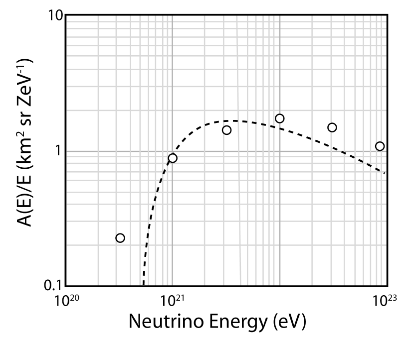
Figure 8: Effective aperture divided by neutrino energy versus energy for GLUE experiment (Gorham et al., 2004) calculated using equation 54 (dotted line) and Monte Carlo calculation of James & Protheroe (2009) for regolith only (open circles, from their Fig. 6a).

5 Summary and Conclusions

Accurate aperture calculations are complicated and laborious and historically have required Monte Carlo simulations. We have shown that an analytic calculation with a series of simplifying approximations can reproduce a result comparable to Monte Carlo simulations, and in addition generate simple scaling laws with a straightforward conceptual interpretation (eq. [54]). We find that it is crucial to account for surface roughness when apertures are intrinsically low, such as when using high frequencies from Earthlike distances, but when the aperture is intrinsically high, such as at low frequencies with high-energy neutrinos, or for lunar orbiters, then surface roughness is of lesser significance. We also find (Fig. [3]) that downward neutrinos significantly dominate over upward neutrinos for higher neutrino energies, and this is especially true for lower frequency observations ($\nu\mathrel{\hbox to0.0pt{\lower 3.0pt\hbox{$\mathchar 536\relax$}\hss}\raise 2.0pt\hbox{$\mathchar 316\relax$}}300$ MHz). However, at the energies nearest to the GZK regime, which is perhaps of greatest cosmological importance, both upward and downward neutrinos may contribute comparably to the detection rate.

These conclusions imply that the first detected GZK neutrino, if detected at high frequency to give a more favorable energy cutoff, may be a downward neutrino whose Cerenkov signal will have escaped by virtue of a lunar roughness feature, or it may with similar likelihood be an upward neutrino that will have made it through a long column of lunar rock and then created an upward Cerenkov flash that did not require assistance from lunar roughness. Alternatively, if the first GZK neutrino detection comes at lower frequency, it will likely be because a downward neutrino sent out a very weak radio signal that did not require lunar surface roughness to escape, but did require an extraordinarily sensitive radio instrument to detect. It is also possible that the first UHE neutrino will come from pion decay near the acceleration region of a UHE proton, and then it could come at an energy well beyond the GZK regime. In that case, the detection could come at low or high frequency, depending on whichever instrument first achieves the necessary sensitivity.

Another important conclusion is that simple scaling laws, with all their extreme portability, may be used to optimize experimental design within a wide range of constraints. They are also useful for making instant comparisons between the apertures of past experiments using a standardized treatment of the relevant input parameters. In this way, the impact of the various inconsistencies between models, such as the detectable Cerenkov cone width, the treatment of transmission and solid-angle magnification, and the role of surface roughness, can be addressed without having to run Monte Carlo simulations with exactly the same parameters. Indeed, uncertainties in the details of such simulations make it difficult for us to resolve several inconsistencies between our results and others quoted in the literature, whether they be due to problems in the Monte Carlo simulations or in our own analytic approximations, especially our use of small-angle approximations and a constant transmission coefficient. For example, we have not been able to determine the source of the order of magnitude increase in the neutrino flux upper limit compared with the published GLUE upper limits (cf. Table 1). This discrepancy was also reported by James & Protheroe (2009) using a Monte Carlo simulation.

One particularly robust result we obtain is that to optimize the detection of neutrinos at a given energy, one should choose a frequency that will yield a value for the $f_{o}$ parameter of roughly 0.8, which implies a ratio of the maximum to the minimum detectable field of about 2, for that energy. Inverting this implies that past experiments at given frequencies are best tailored to the neutrino energies for which the maximum field generated in the telescope by neutrinos of that energy is about twice the minimum detectable field for that instrument.

We would like to acknowledge helpful discussions with Hallsie Reno, John Ralston, and Clancy James, who were especially helpful guides in areas of this effort outside our own expertise.

6 Appendix A: The effective neutrino extinction pathlength

When UHE neutrinos strike the Moon, there is a roughly 1/3 chance (Reno, 2005) that they will initiate via the neutral current interaction a hadronic cascade that will leave roughly 80% of the neutrino energy still in the highly forward-scattered neutrino. The remaining 2/3 of the time, a charged current interaction will destroy the neutrino, but still result in the same roughly 20% of the energy going into the hadronic cascades we wish to detect. Thus from the point of view of detecting the cascade, we do not care whether the interaction was via neutral or charged current. However, this is a relevant question when considering whether or not the neutrino survives the encounter and can initiate further cascades.

Since the observed radio signals are from a narrow layer at the surface, it is highly unlikely that the same neutrino could be involved in multiple detectable showers. Nevertheless, some of the neutrinos we are hoping to detect (labeled the “upward” neutrinos) may have to make their way through a considerable amount of lunar material before arriving at their observable shower location. For these neutrinos, it does matter if they can survive prior neutral-current interactions, losing only $\sim 20$% of their energy each time. For example, a neutrino that suffers two neutral-current interactions and no charge-current interactions can arrive in the domain of interest with roughly 64% of its energy intact, so at the energy of interest, this just means that there can be a contribution from initially higher energy neutrinos. This “downgrading” effect is easily accounted for by increasing the effective neutrino extinction path over and above $L_{\nu}(E)$, by a factor that depends on the steepness of the energy spectrum, thereby increasing the number of “upward” neutrinos that contribute to the aperture at any given energy. Once this has been accounted for, the actual reaction rates for a given neutrino population are still proportional to $L_{\nu}^{-1}$, so the effect is not the same as a global correction to $L_{\nu}$, it is merely an effective reduction in neutrino extinction at energy $E$.

Here we derive in the simplest case the enhancement in the effective extinction pathlength, so we find the factor $\psi$ we use to multiply ${L_{\nu}}(E)$ in eqs. (27) and (37), for a power-law neutrino energy distribution, with flux per unit energy $I(E)\propto E^{-2}$. The power-law nature of the problem imposes a scale invariance that allows us to seek a constant factor by which all effective extinction lengths are altered, where the extinction of $I(E)$ must be modified by the appearance in $I(E)$ of downgraded neutrinos from initially higher energies. This results in an effective extinction coefficient ${\bar{\chi}(E)}$, differing from the actual extinction coefficient $\chi(E)$, such that $I(s)=I_{o}e^{-{\bar{\chi}}s}$. The net extinction over length $ds$ must obey

$${dI\over ds}\ =\ -\chi(E)I_{o}e^{-{\bar{\chi}}s}\ +\ b\cdot 1.077\cdot 0.8\cdot\chi(E)I_{o}e^{-{\bar{\chi}}s}\ ,$$ (69)

where $b$ is the branching ratio for the survival of the neutrino, which here is $b=1/3$ (Cooper-Sarkar & Sarkar, 2008), 1.077 comes from assuming that $\chi(E)\propto E^{1/3}$ so the $\chi$ for the downgraded neutrinos is slightly higher than $\chi(E)$, and the 0.8 factor comes from the combination of the $E^{-2}$ neutrino power law (assumed only for simplicity here) and the fact that higher energy bins are squeezed into narrower energy bins when 20% of the neutrino energy is lost to the hadronic shower.

It remains only to note that the above equation takes on the desired form

$${dI\over ds}\ =\ -{\bar{\chi}}I_{o}e^{-{\bar{\chi}}s}$$ (70)

when ${\bar{\chi}}=\chi/1.4$. Hence, the extinction of neutrinos with $I(E)\propto E^{-2}$ acts as though the extinction length was larger by a factor $\psi=1.4$. Had we instead used a power law of -2.7 instead of -2, the factor would have been 1.3, but the factor could be higher for flatter spectra, such as in the rising hump of the GZK cutoff region. It is even possible for the neutrino flux at a given energy at the start of the GZK hump to experience a region of neutrino enhancement inside the Moon, but we do not deal with this possibility here because no suitably general assumptions about the shape of the neutrino spectrum can be applied at this time. If GZK neutrinos are detected, they will likely come at energies near the peak or the falling part of the GZK hump, so we are probably not underestimating the neutrino population that is being passed down from higher energies as they cross lunar rock.

References

- Alvarez-Muniz & Zas (2001) Alvarez-Muniz, J., & Zas, E. 2001, Radio Detection of High Energy Particles, AIP Conference Proceedings, 579, 128
- Bahcall & Waxman (2001) Bahcall, J., & Waxman, E. 2001, Physical Review D, 64
- Beresnyak (2003) Beresnyak, A. R. 2003, astro-ph/0310295v2
- Beresnyak et al. (2005) Beresnyak, A. R., Dagkesamanskii, R. D., Zheleznykh, I. M., Kovalenko, A. V., & Oreshko, V. V. 2005, Astronomy Reports, 49, 127
- Buitink et al. (2008) Buitink, S., Bacelar, J., Braun, R., de Bruyn, G., Falcke, H., Scholten, O., Singh, K., Stappers, B., Strom, R., & Yahyaoui, R. a. 2008, ArXiv e-prints, 0808
- Cooper-Sarkar & Sarkar (2008) Cooper-Sarkar, A., & Sarkar, S. 2008, Journal of High Energy Physics, 01, 75
- Gandhi et al. (1998) Gandhi, R., Quigg, C., Reno, M. H., & Sarcevic, I. 1998, Physical Review D, 58
- Gorham et al. (2004) Gorham, P. W., Hebert, C. L., Liewer, K. M., Naudet, C. J., Saltzberg, D., & Williams, D. 2004, Physical Review Letters, 93
- Gorham et al. (2001) Gorham, P. W., Liewer, K. M., Naudet, C. J., Saltzberg, D. P., & Williams, D. R. 2001, ArXiv Astrophysics e-prints
- Greisen (1966) Greisen, K. 1966, Phys. Rev. Lett., 16, 748
- Gusev et al. (2006) Gusev, G. A., Lomonosov, B. N., Pichkhadze, K. M., Polukhina, N. G., Ryabov, V. A., Saito, T., Sysoev, V. K., Feinberg, E. L., Tsarev, V. A., & Chechin, V. A. 2006, Cosmic Research, 44, 19
- Hankins et al. (1996) Hankins, T. H., Ekers, R. D., & O’Sullivan, J. D. 1996, Monthly Notices of the Royal Astronomical Society, 283, 1027
- James et al. (2007a) James, C. W., Crocker, R. M., Ekers, R. D., Hankins, T. H., O’Sullivan, J. D., & Protheroe, R. J. 2007a, Monthly Notices of the Royal Astronomical Society, 379, 1037
- James et al. (2007b) —. 2007b, Monthly Notices of the Royal Astronomical Society, 379, 1037
- James & Protheroe (2009) James, C. W., & Protheroe, R. J. 2009, Astroparticle Physics, 30, 318
- Kalashev et al. (2002) Kalashev, O. E., Kuzmin, V. A., Semikoz, D. V., & Sigl, G. 2002, Physical Review D, 66
- Lehtinen et al. (2004) Lehtinen, N. G., Gorham, P. W., Jacobson, A. R., & Roussel-Dupre, R. A. 2004, Physical Review D, 69
- Reno (2005) Reno, M. H. 2005, Nuclear Physics B Proceedings Supplements, 143, 407
- Scholten et al. (2006) Scholten, O., Bacelar, J., Braun, R., de Bruyn, A. G., Falcke, H., Stappers, B., & Strom, R. G. 2006, Astroparticle Physics, 26, 219
- Shepard et al. (1995) Shepard, M. K., Brackett, R. A., & Arvidson, R. E. 1995, Journal of Geophysical Research, 100, 11709
- Williams (2004) Williams, D. R. 2004, Ph.D. Thesis
- Zatsepin & Kuz’min (1966) Zatsepin, G. T., & Kuz’min, V. A. 1966, Soviet Journal of Experimental and Theoretical Physics Letters, 4