Variational approximations of bifurcations of asymmetric solitons in cubic–quintic nonlinear Schrödinger lattices

Abstract.

Using a variational approximation we study discrete solitons of a nonlinear Schrödinger lattice with a cubic-quintic nonlinearity. Using an ansatz with six parameters we are able to approximate bifurcations of asymmetric solutions connecting site-centered and bond-centered solutions and resulting in the exchange of their stability. We show that the numerically exact and variational approximations are quite close for solitons of small powers.

C. Chong

Fakultät für Mathematik, Universität Karlsruhe

Karlsruhe 76128, Germany

D.E. Pelinovsky

Department of Mathematics, McMaster University

Hamilton, Ont., Canada L8S 4K1

1. Introduction

The variational approximation (VA) has long been used as a semi-analytic technique to approximate solitary wave solutions of nonlinear evolution equations with an underlying Hamiltonian structure [13]. There have been a number of papers exploring the VA with four parameters as a relevant approximation of localized modes in discrete nonlinear Schrödinger (DNLS) equations [6, 14, 19]. Kaup [10] extended the variational approximation with six parameters that allowed him to construct not only site-centered solutions (also called on-site solitons) from [14] but also the bond-centered solutions (solitons centered at a midpoint between two adjacent sites also known as inter-site solitons).

Site-centered and bond-centered solitons were recently considered in the context of the DNLS equations with competing cubic focusing and quintic defocusing nonlinearities both in the space of one [3] and two [4] lattice dimensions. It was found that the two branches exchange their stability while continued with respect to the underlying parameters. A salient feature of this stability exchange is that the two branches of site-centered and bond-centered solitions do not intersect directly but are connected by an intermediate branch of asymmetric solitons. It was argued in [4] that the discrete solitons have enhanced mobility near the regimes of stability inversion. These properties were originally discovered in the DNLS equations with a saturable nonlinearity both in the space of one [8] and two [20] dimensions as well as for the DNLS equations with on-site and next-site cubic nonlinearities in the space of one dimension [18]. It was recently shown for the same model in the space of two dimensions [17] that stability inversion and asymmetric solutions may not lead to enhanced mobility of discrete solitons if the bifurcation points of the solution branches are widely separated in the parameter space.

It is the purpose of this work to apply Kaup’s variational method with six parameters from [10] to explain bifurcations of asymmetric solutions and stability exchange of site-centered and bond-centered discrete solitons in the context of the one-dimensional cubic–quintic DNLS equation. In this sense, our work is a complement to the previous paper [3] where discrete solitons were constructed numerically using a dynamical reduction. Dark solitons and staggered solutions of the cubic–quintic DNLS equation were recently studied numerically in Refs. [15] and [16] respectively.

We consider a discrete nonlinear Schrödinger equation with a cubic–quintic nonlinearity in the form,

$$i\dot{\psi}_{n}+C(\psi_{n+1}+\psi_{n-1}-2\psi_{n})+B|\psi_{n}|^{2}\psi_{n}-Q|\psi_{n}|^{4}\psi_{n}=0,\quad n\in\mathbb{Z},$$ (1)

where $\psi_{n}(t):\mathbb{R}_{+}\to\mathbb{C}$ and $(C,B,Q)$ are real-valued parameters. Nonlinear Schrödinger lattices have proved to be relevant models in a variety of contexts (see reviews in [7, 11]), including the description of optical pulses in one-dimensional waveguide arrays [5]. In this application, the quantity $|\psi_{n}|^{2}$ represents the intensity of the electric field of waveguide $n$, $C>0$ represents coupling strength between adjacent waveguides and $(B,Q)$ measure the nonlinearity strength. A large portion of the literature is dedicated to Eq. (1) with $Q=0$, which would correspond to a medium with a Kerr nonlinearity. Recent experimental results [2, 9, 21] have shown that the nonlinear response of some materials is better fit with an additional competing quintic nonlinearity, i.e. $B,Q>0$. This lends relevance to studying the cubic-quintic DNLS equation in the form (1).

The cubic–quintic DNLS equation (1) has two conserved quantities, namely the power,

$$M=\sum_{n\in\mathbb{Z}}|\psi_{n}|^{2},$$ (2)

and the Hamiltonian,

$$H=\sum_{n\in\mathbb{Z}}C\left(\psi^{*}_{n}\psi_{n+1}+\psi_{n}\psi^{*}_{n+1}-2|\psi_{n}|^{2}\right)+\frac{B}{2}|\psi_{n}|^{4}-\frac{Q}{3}|\psi_{n}|^{6}.$$ (3)

Steady-state solutions have the form $\psi_{n}=u_{n}e^{-i\mu t}$, $n\in\mathbb{Z}$, where $\mu\in\mathbb{R}$ and $u_{n}\in\mathbb{R}$ are found from the stationary DNLS equation,

$$\mu u_{n}+C(u_{n+1}+u_{n-1}-2u_{n})+Bu_{n}^{3}-Qu_{n}^{5}=0,\quad n\in\mathbb{Z}.$$ (4)

We seek localized solutions of the stationary DNLS equation (4) which in turn correspond to discrete solitons.

Spectral stability of the steady-state solutions is studied with the linearization ansatz,

$$\psi_{n}(t)=\left(u_{n}+(v_{n}+iw_{n})e^{\lambda t}+(v^{*}_{n}+iw^{*}_{n})e^{\lambda^{*}t}\right)e^{-i\mu t},\quad n\in\mathbb{Z},$$

which leads to the spectral problem,

$$\left\{\begin{array}[]{cc}-\mu v_{n}-C(v_{n+1}+v_{n-1}-2v_{n})-3Bu_{n}^{2}v_{n}+5Qu_{n}^{4}v_{n}=-\lambda w_{n},\\ -\mu w_{n}-C(w_{n+1}+w_{n-1}-2w_{n})-Bu_{n}^{2}w_{n}+Qu_{n}^{4}w_{n}=\lambda v_{n},\end{array}\right.\quad n\in\mathbb{Z}.$$ (5)

We are looking for nonzero solutions of the linearized system in $L^{2}(\mathbb{Z},\mathbb{C}^{2})$ called eigenvectors. The steady-state solution is called unstable if there exists at least one eigenvector for which ${\rm Re}(\lambda)>0$. Otherwise, the solution is called spectrally stable.

Steady-state solutions are considered in Section 2. Spectral stability of these solutions is studied in Section 3. For both problems, we compare results of the variational approximations and the direct numerical approximations.

2. Variational approximations of the steady-state solutions

Solutions of the DNLS equation (1) correspond to critical points of the Lagrangian,

$$\mathcal{L}=\sum_{n\in\mathbb{Z}}\frac{i}{2}\left(\psi^{*}_{n}\partial_{t}\psi_{n}-\psi_{n}\partial_{t}\psi^{*}_{n}\right)+C\left(\psi^{*}_{n}\psi_{n+1}+\psi_{n}\psi^{*}_{n+1}-2|\psi_{n}|^{2}\right)+\frac{B}{2}|\psi_{n}|^{4}-\frac{Q}{3}|\psi_{n}|^{6}.$$ (6)

To find approximate solutions for discrete solitons, we pose a trial function in the form,

$$\psi_{n}=Ae^{i\phi_{n}}e^{-\eta|n-n_{0}|},\quad\phi_{n}=\alpha+k(n-n_{0})+\frac{\beta}{2}(n-n_{0})^{2},$$ (7)

where each of the six parameters are dependent on $t$. Substituting Eq. (7) into the Lagrangian (6) and evaluating the sums yields the effective Lagrangian,

$$\mathcal{L}_{\mathrm{eff}} = -A^{2}\left(\frac{\mathrm{d}\alpha}{\mathrm{d}t}-\frac{k}{2}\frac{\mathrm{d}\chi}{\mathrm{d}t}\right)S_{0}-A^{2}\left(\frac{\mathrm{d}k}{\mathrm{d}t}-\frac{\beta}{2}\frac{\mathrm{d}\chi}{\mathrm{d}t}\right)S_{1}-\frac{A^{2}}{2}\frac{\mathrm{d}\beta}{\mathrm{d}t}S_{2}$$ (8)

$$+CA^{2}\left(e^{ik}S_{\beta}+e^{-ik}S_{\beta}^{*}-2S_{0}\right)+\frac{B}{2}A^{4}S_{4}-\frac{Q}{3}A^{6}S_{6},$$

where $\chi=2n_{0}-1$ and,

$$S_{0}(\eta,\chi) = {\frac{\cosh\chi\eta}{\sinh\eta}},$$

$$S_{1}(\eta,\chi) = \frac{\cosh\eta\sinh\chi\eta}{2\sinh^{2}\eta}+\frac{\chi}{2}S_{0},$$

$$S_{2}(\eta,\chi) = \left(\frac{2}{\sinh^{2}\eta}+\frac{1}{4}\right)S_{0}-\frac{\chi}{2}\frac{\cosh\eta\sinh\chi\eta}{\sinh^{2}\eta}-\frac{\chi^{2}}{4}S_{0},$$

$$S_{4}(\eta,\chi) = S_{0}(2\eta,\chi),$$

$$S_{6}(\eta,\chi) = S_{0}(3\eta,\chi),$$

$$S_{\beta}(\eta,\chi,\beta) = e^{-\eta}e^{-\frac{i}{2}\beta\chi}\left(1+\frac{e^{-\eta\chi}}{e^{i\beta}e^{\eta}-e^{-\eta}}+\frac{e^{\eta\chi}}{e^{-i\beta}e^{\eta}-e^{-\eta}}\right).$$

Since the center $n_{0}$ of the ansatz (7) can be arbitrarily chosen on $[0,1]$ module the discrete group of translations in $n\in\mathbb{Z}$, we shall consider $\chi$ on $[-1,1]$ (this restriction was used already in the derivation of (8)). The solution with $\chi=0$ is centered between lattice sites and hence is called bond-centered. The solution with $\chi=\pm 1$ is centered on a lattice site and hence is called site-centered. Solutions for $\chi\in(-1,0)\cup(0,1)$ are called asymmetric.

According to the variational principle, the effective Lagrangian $\mathcal{L}_{\mathrm{eff}}$ achieves critical values at the Euler-Lagrange equations,

$$\frac{\partial\mathcal{L}_{\mathrm{eff}}}{\partial p_{j}}-\frac{d}{dt}\left[\frac{\partial\mathcal{L}_{\mathrm{eff}}}{\partial\dot{p}_{j}}\right]=0,$$ (9)

where $p_{j}$ represents a parameter of ansatz (7). Varying $\alpha$ yields the conservation law,

$$A^{2}S_{0}=M,$$ (10)

which corresponds to the dynamical invariant (2) of the power. Varying $A$ yields,

$$\frac{\mathrm{d}\alpha}{\mathrm{d}t} = \frac{\mathrm{d}\chi}{\mathrm{d}t}\frac{k}{2}-\frac{\mathrm{d}k}{\mathrm{d}t}\frac{S_{1}}{S_{0}}+\frac{\beta}{2}\frac{S_{1}}{S_{0}}\frac{\mathrm{d}\chi}{\mathrm{d}t}-\frac{1}{2}\frac{\mathrm{d}\beta}{\mathrm{d}t}\frac{S_{2}}{S_{0}}+\frac{C}{S_{0}}(e^{ik}S_{\beta}+e^{-ik}S_{\beta}^{*}-2S_{0})$$ (11)

$$\;+BM\frac{S_{4}}{S_{0}^{2}}-QM^{2}\frac{S_{6}}{S_{0}^{3}}\;.$$

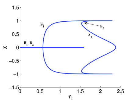
Figure 1. Solutions of Eqs. (12) and  (2) for $C=0.1$, $B=2$, and $Q=1$.

Before writing the remaining equations, it will be more convenient to make use of the fact that we seek steady-state solutions. This corresponds to

$$\beta=k=\frac{\mathrm{d}\chi}{\mathrm{d}t}=\frac{\mathrm{d}\eta}{\mathrm{d}t}=0\quad\mbox{\rm and}\quad\frac{d\alpha}{dt}=-\mu,$$

where $\mu$ is the parameter of the steady-state solution. With this assumption, the equations corresponding to variation of $k$ and $\beta$ are identically satisfied. Varying $\chi$ and $\eta$ and making use of Eq. (11) leads to the following two equations respectively,

$$\frac{A^{2}\eta\sinh\eta\chi}{\sinh\eta\cosh\eta\chi}\left(\frac{A^{4}2Q\cosh\eta\cosh\eta\chi}{4\cosh^{2}\eta-1}-A^{2}+Ce^{-\eta}\sinh 2\eta\right)=0,$$ (12)

and,

$$-Ce^{-\eta}\left(1+\frac{\cosh\eta\chi-\cosh\eta}{\sinh\eta}+\frac{\chi\sinh\eta\chi}{\cosh\eta\chi}\right)+\frac{BA^{2}\chi\sinh\eta\chi}{2\sinh 2\eta\cosh\eta\chi}$$

$$+\frac{BA^{2}\cosh 2\eta\chi}{2\sinh^{2}2\eta}-QA^{4}\left(\frac{\chi\sinh\eta\chi}{\sinh 3\eta}+\frac{\cosh\eta\cosh 3\eta\chi}{\sinh^{2}3\eta}\right)=0.$$

Note these equations with $Q=0$ correspond to those in Ref. [10]. When $\chi=0$ (bond-centered solutions), Eq. (12) is identically satisfied and Eq. (2) becomes,

$$\frac{-Ce^{-\eta}(1+e^{-\eta})\sinh^{2}2\eta}{\sinh\eta}+\frac{BA^{2}}{2}-\frac{QA^{4}\cosh\eta\sinh^{2}2\eta}{\sinh^{2}3\eta}=0,$$ (14)

which is easily solved for $A^{2}$, giving an existence condition in terms of the parameter $\eta$. There exists exactly two bond-centered solutions (denoted by $B_{1}$ and $B_{2}$) for $\eta\in(0,\eta_{\rm cr})$, which disappear as a result of the saddle–node bifurcation at $\eta=\eta_{\rm cr}$. See Fig. 1, where solutions of Eqs. (12) and (2) are plotted for $C=0.1$, $B=2$, and $Q=1$ with $\eta_{\rm cr}\approx 1.56$. We note, for larger $C$ steady-state solutions become smoother (they approach the continuous counterpart) and so the ansatz (7), which is based on an exponential cusp, becomes irrelevant.

For $\chi\neq 0$, the term in parenthesis of Eq. (12) can be used as condition for $A^{2}$, which can then be substituted into (2) yielding a root finding problem in $(\eta,\chi)$ parameter space. We find exactly three pairs of solutions for $C=0.1$, $B=2$, and $Q=1$, which are denoted by $S_{1}$,$S_{2}$, and $A_{1}$ in Fig. 1. Branches $(S_{1},S_{2})$ and $(S_{2},A_{1})$ are connected by means of the saddle-node bifurcations. Branch $S_{1}$ arises from $\chi=0$ as a result of the supercritical pitchfork bifurcation, while branches $S_{2}$ and $A_{1}$ arise from $\chi=0$ as a result of the subcritical pitchfork bifurcation.

The solution branches $S_{1}$ and $S_{2}$ approach $\chi=1$ rapidly, so that they correspond to the site-centered solitons slightly disturbed by the variational approximation. The solution branch $A_{1}$ is a true asymmetric solution that connects the bond-centered and site-centered solitons. Only one branch $S_{1}$ of site-centered solutions and only one branch $B_{1}$ of bond-centered solutions exist in the cubic case $Q=0$, where these two branches extend for any $\eta>0$.

To test the validity of the variational approximations we compare them against direct numerical solutions of the stationary DNLS equation (4). The “numerically exact” solutions are obtained using a Newton method with the VA solutions as initial seeds. The profiles of the discrete solitons that are obtained via the VA and the corresponding numerical solutions are shown in Fig. 2.

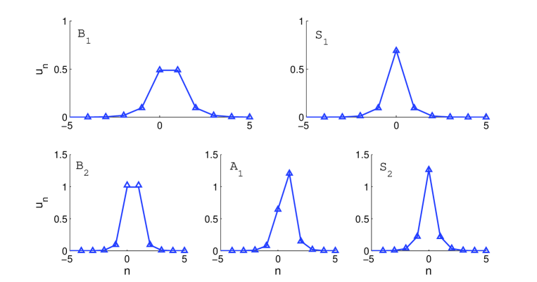
Figure 2. Plot of numerical (solid lines) and variational (markers) solutions for $C=0.1$, $B=2$, $Q=1$. Top: Short bond-centered (left) and site-centered (right) solutions. Bottom: A taller bond-centered (left) and site-centered (right) solution. The asymmetric solution (middle) is an intermediate between the two symmetric profiles. The labels $A_{1}$, $B_{1}$, $B_{2}$, $S_{1}$, and $S_{2}$ correspond to those in Fig. 1.

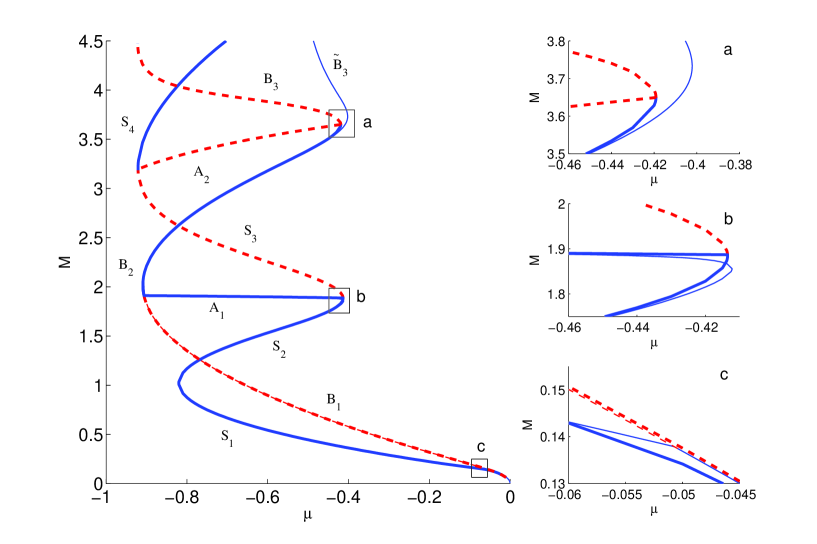
Figure 3. (Color online) Plot of the power $M$ of the VA solutions (thin lines) and numerical solutions (thick lines). Stable branches are represented by solid blue lines and unstable branches by dashed red lines. There are two principle branches, one corresponding to site-centered solutions (labeled $S_{j},\,j=1..4$) and one for bond-centered solutions (labeled $B_{j},\,j=1..3$). The two principle branches are connected via asymmetric solutions (labeled $A_{j},\,j=1,2$) at points of stability change. Only the branches $S_{1},S_{2},A_{1},B_{1},$ and $B_{2}$, are captured by the VA. Differences between the VA and numerical solutions are more visible in the zooms labeled ‘a’, ‘b’ and ‘c’. The branch labeled $\tilde{B}_{3}$ corresponds to the VA that fails to capture $B_{3}$.

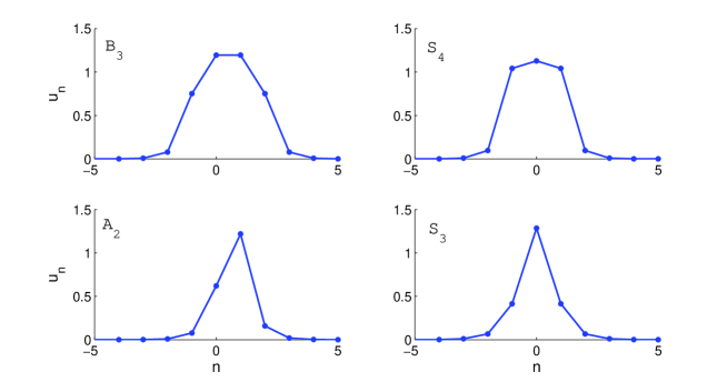
Figure 4. Examples of numerical solutions shown in Fig. 3 that the VA did not capture. The failure of the VA is due to the wide nature of the solutions. Parameter values are $C=0.1$, $B=2$, and $Q=1$.

It is more instructive for comparison to plot the solution branches in the $(\mu,M)$ plane, where $M$ is defined in Eq. (10) and $\mu=-\frac{d\alpha}{dt}$, see Fig. 3. The predicted stability is also depicted (see Sec. 3 for details on stability computations).

Besides the five solutions predicted within the variational approximation, there exists additional branches $S_{3}$, $S_{4}$, $B_{3}$, $A_{2}$ of solutions of Eq. (4) that appear on Fig. 3. See Fig. 4 for profiles of these “wide” solutions. The pattern of Fig. 3 suggests existence of an infinite number of additional branches of discrete solitons for large power $M$ with a characteristic snaking behavior. The snaking behavior was also found in the higher dimensional cubic-quintic DNLS equation [4] and the Swift-Hohenberg equation [1, 12]. It seems the role a higher order dispersion plays in the Swift-Hohenberg equation is replaced by discreteness in the cubic-quintic DNLS equation.

The bifurcations shown in Fig. 3 look as if the asymmetric solutions connect exactly at the turning points of bond-centered or site-centered solutions. This is not the case. Rather, there exists a pair of saddle–node and pitchfork bifurcations and the stability exchange occurs at the pitchfork bifurcation where the asymmetric solutions emanate. Interestingly, the VA is able to accurately capture this subtle bifurcation scenario. In Fig. 5 a plot of such a bifurcation pair is shown. This particular pair represents a saddle-node bifurcation of a short ($B_{1}$) and tall ($B_{2}$) bond-centered solution and a pitchfork of two asymmetric solutions ($A_{1}$) and the short bond-centered solution ($B_{1}$). The agreement between the variational and numerical approximations is impressive. The stability is also correctly predicted.

On the other hand, bifurcations including the site-centered solutions are not captured as well. This should not be surprising since site-centered solutions are never truly represented by the VA (see Fig. 1). We point out other minor discrepancies between the variational approximations and the numerical results in the zooms of Fig. 3. Zoom (a) shows where the VA solution $\tilde{B}_{3}$ departs from the corresponding numerical solution $B_{3}$. This is expected as the ansatz (7) is only valid for “narrow” solutions, i.e. those that have at most two initially excited sites. Zoom (b) shows that the asymmetric solution $A_{1}$ is connected to the site-centered solution $S_{2}$ (opposed to $S_{3}$) and is underestimated. The wider short site-centered solution $S_{3}$ is not captured at all by the VA (as expected). Finally, zoom (c) shows that the VA falsely predicts collision of the bond-centered $B_{1}$ and site-centered $S_{1}$ solutions for a non-zero value of $M$, similar to the cubic case discussed by Kaup in [10].

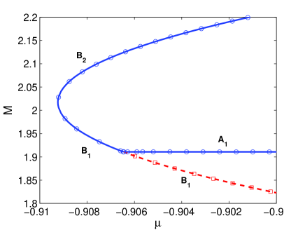
Figure 5. Plot of numerical (lines) and variational (markers) approximations of power $M$ versus $\mu$ for $C=0.1$, $B=2$, $Q=1$ in a parameter region near a pitchfork bifurcation. Stable solutions of the VA are indicated by circles and unstable solutions by squares.

3. Variational approximations of spectral stability

In order to determine stability within the VA we return to the variational equations (9) but this time without the assumption that $\beta=k=\frac{\mathrm{d}\chi}{\mathrm{d}t}=\frac{\mathrm{d}\eta}{\mathrm{d}t}=0$. Let $\vec{x}=(\beta,\chi,\eta,k)^{T}$ represent the four parameters of ansatz (7) after Eqs. (10) and (11) are used. To perform a linear stability analysis we substitute,

$$\vec{x}=\vec{x}_{0}+\epsilon\vec{y}e^{\lambda t},\quad\lambda\in\mathbb{C},$$

into the four variational equations, where the steady-state solution is defined by $\vec{x}_{0}=(0,\chi_{0},\eta_{0},0)^{T}$ and $(\chi_{0},\eta_{0})$ satisfy Eqs. (12) and (2). Keeping only the terms linear in $\epsilon$ leads to the generalized eigenvalue problem,

$$\lambda{\bf A}\vec{y}={\bf B}\vec{y},$$ (15)

where the entries of the $4\times 4$ matrices ${\bf A}$ and ${\bf B}$ are given by,

$$a_{11} =0, a_{21} =0,$$

$$a_{12} =\frac{M}{2}+M\frac{\partial}{\partial\chi}\left[\frac{S_{1}}{S_{0}}\right], a_{22} =\frac{M}{2}\left(\frac{S_{1}}{S_{0}}+\frac{\partial}{\partial\chi}\left[\frac{S_{2}}{S_{0}}\right]\right),$$

$$a_{13} =M\frac{\partial}{\partial\eta}\left[\frac{S_{1}}{S_{0}}\right], a_{23} =\frac{M}{2}\frac{\partial}{\partial\eta}\left[\frac{S_{2}}{S_{0}}\right],$$

$$a_{14} =0, a_{24} =0,$$

$$a_{31} =\frac{M}{2S_{0}}\left(\frac{\partial S_{0}}{\partial\chi}\frac{S_{2}}{S_{0}}-\frac{\partial S_{2}}{\partial\chi}-S_{1}\right), a_{41} =\frac{M}{2S_{0}}\left(\frac{\partial S_{0}}{\partial\eta}\frac{S_{2}}{S_{0}}-\frac{\partial S_{2}}{\partial\eta}\right),$$

$$a_{32} =0, a_{42} =0,$$

$$a_{33} =0, a_{43} =0,$$

$$a_{34} =\frac{M}{S_{0}}\left(\frac{\partial S_{0}}{\partial\chi}\frac{S_{1}}{S_{0}}-\frac{\partial S_{1}}{\partial\chi}\right)-\frac{M}{2}, a_{44} =\frac{M}{S_{0}}\left(\frac{\partial S_{0}}{\partial\eta}\frac{S_{1}}{S_{0}}-\frac{\partial S_{1}}{\partial\eta}\right),$$

and,

$$b_{11} =\frac{CM}{S_{0}}\left(\frac{\sinh\eta\chi}{\sinh^{2}\eta}-\chi e^{-\eta}(1+S_{0})\right), b_{21} =\frac{-CM}{S_{0}}\left(\frac{\partial^{2}S_{\beta}}{\partial\beta^{2}}+\frac{\partial^{2}S_{\beta}^{*}}{\partial\beta^{2}}\right),$$

$$b_{12} =0, b_{22} =0,$$

$$b_{13} =0, b_{23} =0,$$

$$b_{14} =\frac{2CM}{S_{0}}e^{-\eta}(1+S_{0}), b_{24} =\frac{CM}{S_{0}}\left(\frac{\sinh\eta\chi}{\sinh^{2}\eta}-\chi e^{-\eta}(1+S_{0})\right),$$

$$b_{31} =0, b_{41} =0,$$

$$b_{32} =-\frac{\partial}{\partial\chi}\left[\frac{\partial L}{\partial\chi}+\frac{\partial S_{0}}{\partial\chi}P\right], b_{42} =-\frac{\partial}{\partial\chi}\left[\frac{\partial L}{\partial\eta}+\frac{\partial S_{0}}{\partial\eta}P\right],$$

$$b_{33} =-\frac{\partial}{\partial\eta}\left[\frac{\partial L}{\partial\chi}+\frac{\partial S_{0}}{\partial\chi}P\right], b_{43} =-\frac{\partial}{\partial\eta}\left[\frac{\partial L}{\partial\eta}+\frac{\partial S_{0}}{\partial\eta}P\right],$$

$$b_{34} =0, b_{44} =0.$$

Here we have defined,

$$L = \frac{CM}{S_{0}}\left(S_{\beta}+S^{*}_{\beta}-2S_{0}\right)+\frac{BM^{2}}{2S_{0}^{2}}S_{4}-\frac{QM^{3}}{3S_{0}^{3}}S_{6},$$

$$P = \frac{-CM}{S_{0}^{2}}\left(S_{\beta}+S^{*}_{\beta}-2S_{0}\right)-\frac{BM^{2}}{S_{0}^{3}}S_{4}+\frac{QM^{3}}{S_{0}^{4}}S_{6},$$

and each entry is evaluated at the fixed point $\vec{x}_{0}$. For the form of the perturbation chosen, an eigenvalue with Re$(\lambda)>0$ indicates instability of the steady-state solution $\vec{x}_{0}$.

Since ${\bf A}$ and ${\bf B}$ are real-valued matrices, both $\lambda$ and $\lambda^{*}$ are eigenvalues. Since ${\bf A}$ and ${\bf B}$ has a clear block structure, if $\lambda$ is an eigenvalue with the eigenvector $\vec{y}$, then $-\lambda$ is an eigenvalue with the eigenvector $S\vec{y}$, where $S={\rm diag}(1,-1,-1,1)$. Therefore, eigenvalues of (15) occur as pairs of real or imaginary eigenvalues or as quartets of complex eigenvalues. A typical example of eigenvalues of (15) is shown on the left panel of Fig. 6 for the unstable solution $B_{1}$ with a pair of real and a pair of imaginary eigenvalues.

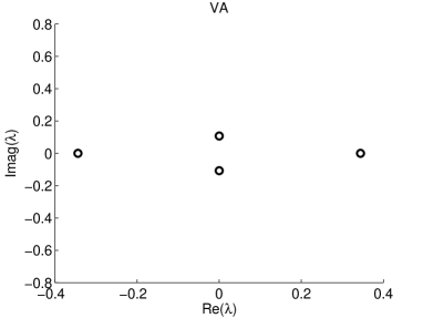
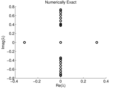
Figure 6. Eigenvalues corresponding to the bond-centered solution $B_{1}$ in the variational system (left) and the full system (right).

The stability of the VA solutions corresponding to Fig. 3 was computed from eigenvalues of the generalized problem (15). The spectrum for each of the variational solutions shown in Fig. 3 is plotted in the left panels of Fig. 7. Only the bond-centered solution $B_{1}$ has a branch that is predicted to be unstable. The bottom left panel of Fig. 7 is a zoom of small eigenvalues in the top left panel. Where the asymmetric solution $A_{1}$ meets the bond-centered solutions $B_{1}$ and $B_{2}$ corresponds to stability exchange, whereas the connection to the site-centered solution $S_{2}$ occurs at $\lambda^{2}<0$ and hence no stability change takes place. Note that each branch of VA solutions has exactly two pairs of real or imaginary eigenvalues of the generalized problem (15).

A linear stability analysis of the “numerically exact” solutions was also carried out from the spectral stability problem (5) using the procedure described in Ref. [3]. The numerical approximation of the spectrum for the unstable bond-centered solution $B_{1}$ is shown on the right panel of Fig. 6. Note that there is always a double zero eigenvalue in the stability problem (5) which is related to the gauge symmetry. This double zero eigenvalue corresponds to the eigenvector $(v_{n},w_{n})=(0,u_{n})$ and the generalized eigenvector $(v_{n},w_{n})=(\partial_{\mu}u_{n},0)$ of system (5). This double zero eigenvalue is captured by the variational approximation and it results in the conservation law (10) and the variational equation (11). On the other hand, the VA gives two pairs of eigenvalues and only the real pair persists in the numerical approximation. The purely imaginary pair of eigenvalues does not exist in the numerical solutions, where it is replaced by the continuous spectral band on the two symmetric intervals of the purely imaginary axis.

Isolated, non-zero eigenvalues for solutions $B_{1}$, $B_{2}$, $S_{2}$, $S_{3}$, and $A_{1}$ are shown in the right panels of Fig. 7. We note that no isolated eigenvalues of $S_{1}$ exist. The overall “look” of the top panels of Fig. 7 are quite similar, but more importantly, the stability is correctly predicted. Note that the right panels of Fig. 7 contains fewer eigenvalues than the left panels of Fig. 7 because some of the purely imaginary eigenvalues of the VA solutions approximate the continuous spectrum of the numerical solutions. An interesting difference is seen in the bottom right panel of Fig. 7. In the full problem, the eigenvalue pair for the asymmetric solution $A_{1}$ vanishes when $A_{1}$ intersects with the site-centered solution $S_{2}$.

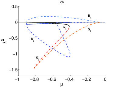
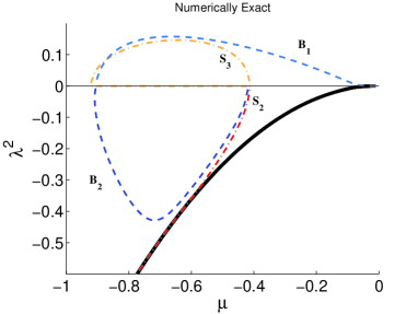
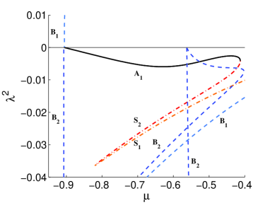
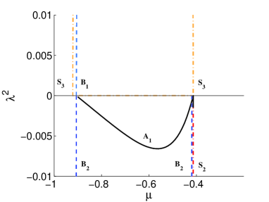
Figure 7. (Color online) Top: plot of eigenvalues for the VA solutions (left) and numerical solutions (right) at $C=0.1$, $B=2$, and $Q=1$. Site-centered branches are plotted as dashed-dot lines (in various shades of red for each branch) and bond-centered branches as dashed lines (in various shades of blue). The asymmetric solution is shown as a solid black line. The thick solid black line shows the boundary of the continuous spectral band in the full problem. Bottom: zooms of the top panels near $\lambda^{2}\approx 0$.

In conclusion, we have extended the results of Ref. [10] to show that not only does the VA faithfully represent the fundamental localized modes, but is also able to correctly predict the corresponding stability for small coupling constant $C$ and power $M$. We showed this in the context of the cubic–quintic DNLS equation, which exhibits a family of discrete solitons, five of which were accurately captured by the variational approximation. It would be interesting to derive the variational equations in the context of time-dependent perturbations, although, the resulting equations would be far more complex and may undermine the utility of the method. It would also be relevant to extend the results of [4] and apply this analysis to the higher dimensional cubic–quintic DNLS equation.

Received xxxx 20xx; revised xxxx 20xx.

References

- [1] M. Beck, J. Knobloch, D.J.B. Lloyd, B. Sandstede, T. Wagenknecht, Snakes, ladders, and isolas of localised patterns, SIAM J. Math. Anal, accepted.
- [2] G. Boudebs, S.Cherukulappurath, H. Leblond, J. Troles, F. Smektala, F. Sanchez, Experimental and theoretical study of higher-order nonlinearities in chalcogenide glasses, Opt. Commun., 219 (2003), 427-433.
- [3] R. Carretero-Gonzáles, J. D. Talley, C. Chong, B.A. Malomed, Multistable solitons in the cubic–quintic discrete nonlinear Schrödinger equation, Physica D, 216 (2006), 77–89.
- [4] C. Chong, R. Carretero-González, B.A. Malomed, P.G. Kevrekidis, Multistable solitons in higher–dimensional cubic–quintic nonlinear Schrödinger lattices, Physica D, 238 (2009), 126–136.
- [5] D. N. Christodoulides, R. I. Joseph, Discrete self-focusing in nonlinear arrays of coupled waveguides, Opt. Lett., 13 (1988), 794-796.
- [6] J. Cuevas, P.G. Kevrekidis, D.J. Frantzeskakis, B.A. Malomed, Discrete solitons in nonlinear Schrödinger lattices with a power-law nonlinearity, Physica D, 238 (2009), 67-76.
- [7] J.Ch. Eilbeck, M. Johansson, The discrete nonlinear Schrödinger equation -20 years on, in “Localization and Energy Transfer in Nonlinear Systems” (eds. L. Vazquez, R.S. MacKay, M.P. Zorzano), World Scientific, (2003), 44-67.
- [8] L. Hadžievski, A. Maluckov, M. Stepić, D. Kip, Power controlled soliton stability and steering in lattices with saturable nonlinearity, Phys. Rev. Lett., 93 (2004), 033901.
- [9] R. A. Ganeev, M. Baba, M. Morita, A. I. Ryasnyansky, M. Suzuki, M. Turu, H. Kuroda, Fifth-order optical nonlinearity of pseudoisocyanine solution at 529 nm, J. Opt. A: Pure Appl. Opt. 6 (2004), 282-287.
- [10] D.J. Kaup, Variational solutions for the discrete nonlinear Schr dinger equation, Math. Comput. Simulat., 69 (2005), 322–333.
- [11] P.G. Kevrekidis, K.Ø. Rasmussen, A.R. Bishop, The discrete nonlinear Schrödinger equation: a survey of recent results, Int. J. Mod. Phys. B, 15 (2001), 2833-2900.
- [12] D.J.B. Lloyd, B. Sandstede, Localized radial solutions of the Swift-Hohenberg equation, Nonlinearity, 22 (2009), 485–524.
- [13] B.A. Malomed, Variational methods in nonlinear fiber optics and related fields, Prog. Opt., 43 (2002), 71-193.
- [14] B.A. Malomed, M.I. Weinstein, Soliton dynamics in the discrete nonlinear Schrödinger equation, Phys. Lett. A, 220 (1996), 91-96.
- [15] A. Maluckov, L. Hadžievski, B. A. Malomed, Dark solitons in dynamical lattices with the cubic-quintic nonlinearity, Phys. Rev. E, 76 (2007), 046605.
- [16] A. Maluckov, L. Hadžievski, B.A. Malomed, Staggered and moving localized modes in dynamical lattices with the cubic-quintic nonlinearity, Phys. Rev. E, 77 (2008), 036604.
- [17] M. Öster, M. Johansson, Stability, mobility and power currents in a two-dimensional model for waveguide arras with nonlinear coupling, Physica D, 238 (2009), 88–99.
- [18] M. Öster, M. Johansson, A. Eriksson, Enhanced mobility of strongly localized modes in waveguide arrays by inversion of stability Phys., Rev. E 67 (2003), 056606.
- [19] I.E. Papacharalampous, P.G. Kevrekidis, B.A. Malomed, D.J. Frantzeskakis, Soliton collisions in the discrete nonlinear Schrödinger equation, Phys. Rev. 68 (2003), 046604.
- [20] R.A. Vicencio, M. Johansson, Discrete soliton mobility in two-dimensional waveguide arrays with saturable nonlinearity, Phys. Rev. E 73 (2006), 046602.
- [21] C. Zhan, D. Zhang, D. Zhu, D. Wang, Y. Li, D. Li, Z. Lu, L. Zhao, Y. Nie, Third- and fifth-order optical nonlinearities in a new stilbazolium derivative, J. Opt. Soc. Am. B, 19 (2002), 369-375.