Length scale dependent diffusion in the Anderson model at high temperatures

Abstract

We investigate a single particle on a $3$-dimensional, cubic lattice with a random on-site potential ($3$D Anderson model). We concretely address the question whether or not the dynamics of the particle is in full accord with the diffusion equation. Our approach is based on the time-convolutionless (TCL) projection operator technique and allows for a detailed investigation of this question at high temperatures. It turns out that diffusive dynamics is to be expected for a rather short range of wavelengths, even if the amount of disorder is tuned to maximize this range. Our results are partially counterchecked by the numerical solution of the full time-dependent Schrödinger equation.

,

Since it had been suggested by P. W. Anderson, the Anderson model served as a paradigm for transport in disordered systems [1, 2, 3, 4, 5, 6]. In its probably simplest form the Hamiltonian may be written as

$$H=\sum_{\bf r}\epsilon_{\bf r}\,a^{\dagger}_{\bf r}\,a_{\bf r}+\sum_{\text{NN}}a^{\dagger}_{\bf r}\,a_{\bf r^{\prime}}\;,$$ (1)

where $a_{\bf r}$, $a^{\dagger}_{\bf r}$ are the usual annihilation, respectively creation operators; $\bf r$ labels the sites of a $d$-dimensional lattice; and NN indicates a sum over nearest neighbors. The $\epsilon_{\bf r}$ are independent random numbers, e.g., Gaussian distributed numbers with mean $\langle\epsilon_{\bf r}\rangle=0$ and variance $\langle\epsilon_{\bf r}\,\epsilon_{\bf r^{\prime}}\rangle=\delta_{{\bf r},{\bf r}^{\prime}}\,\sigma^{2}$. Thus, the first sum in Eq. (1) describes a random on-site potential and hence disorder.

The phenomenon of localization, including localization lengths, has intensively been studied in this system [1, 2, 3, 4]. For the lower dimensional cases $d=1$ and $d=2$ (in the thermodynamic limit, i.e., with respect to the infinite length scale) an insulator results for arbitrary (non-zero) values of $\sigma$, see, e.g., Ref. [4]. Of particular interest is the $3$-dimensional case. Here, at zero temperature, increasing disorder induces a metal-to-insulator transition at the infinite length scale [3, 4]. However, with respect to finite length scales the following transport types are generally expected: i.) ballistic on a scale below some, say, mean free path; ii.) possibly diffusive on a scale above this mean free path but below the localization length; iii.) localized (isolating) on a scale above the localization length. In the above transition decreasing disorder is viewed to reduce the size of the third regime, until it vanishes.

Here, other than most of the pertinent literature, we do not focus on the mere existence of a finite localization length. We rather concentrate on the size of the intermediate regime and the dynamics within. We demonstrate that it is indeed diffusive (rather than subdiffusive, superdiffusive, or anything else). In principle, for long localization lengths (or no localization) this regime could be very large. But the results presented in the paper at hand indicate that it is not, at least not in the limit of high temperatures. Investigations in that direction (but not for $d=3$) are also performed in Refs. [6, 7].

Our approach is based on the time-convolutionless (TCL) projection operator technique [8] which has already been applied to the transport properties of similar models without disorder [9, 10, 11, 12]. In its simplest form (which we apply here) this method is restricted to the infinite temperature limit. This implies that energy dependences are not resolved, i.e., our results are to be interpreted as results on an overall behavior of all energy regimes.

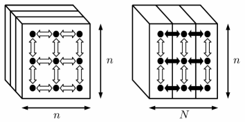
Figure 1: A $3$-dimensional lattice which consists of $N$ layers with $n\times n$ sites each. Only next-neighbor hoppings are taken into account. Intra-layer hoppings are specified by a constant $\alpha=1$ (white arrows), inter-layer hoppings by another constant $\beta$ (black arrows).

As shown in Fig. 1, we consider a $3$-dimensional lattice consisting of $N$ layers with $n\times n$ sites each. The Hamiltonian of our model is almost identical to Eq. (1) with one single exception: All hopping terms that correspond to hoppings between layers (black arrows in Fig. 1) are multiplied by some constant $\beta$. This is basically done due to technical reasons, see below. However, for $\beta=1$ the Hamiltonian reduces to the standard Anderson Hamiltonian (1).

We now establish a “coarse-grained” description in terms of subunits: At first we take all those terms of the Hamiltonian which only contain the sites of the $\mu$th layer in order to form the local Hamiltonian $h_{\mu}$ of the subunit $\mu$. Thereafter all those terms which contain the sites of adjacent layers $\mu$ and $\mu+1$ are taken in order to form the interaction $\beta\,v_{\mu}$ between neighboring subunits $\mu$ and $\mu+1$. Then the total Hamiltonian may be also written as $H=H_{0}+\beta\,V$,

$$H_{0}=\sum_{\mu=0}^{N-1}h_{\mu}\,,\quad V=\sum_{\mu=0}^{N-1}v_{\mu}\;,$$ (2)

where we employ periodic boundary conditions, e.g., we identify $\mu=N$ with $\mu=0$. The above introduction of the additional parameter $\beta$ thus allows for the independent adjustment of the “interaction strength”. We are going to work in the interaction picture. The hence indispensable eigenbasis of $H_{0}$ may be found from the diagonalization of disconnected layers.

By $\Pi_{\mu}$ we denote the particle number operator of the $\mu$th subunit, i.e., the sum of $a^{\dagger}_{\bf r}\,a_{\bf r}$ over all ${\bf r}$ of the $\mu$th layer. Since $[\sum_{\mu}\Pi_{\mu},H]=0$, the one-particle subspace may be analyzed separately, which will be done throughout this work.

The total state of the system is naturally represented by a time-dependent density matrix $\rho(t)$. Consequently, the quantity $P_{\mu}(t)\equiv\text{Tr}\{\,\rho(t)\,\Pi_{\mu}\,\}$ is the probability for locating the particle somewhere within the $\mu$th subunit. The consideration of these “coarse-grained” probabilities corresponds to the investigation of transport along the direction which is perpendicular to the layers. Instead of simply characterizing whether or not there is transport at all, we analyze the full dynamics of the $P_{\mu}$.

Those dynamics may be called diffusive, if the $P_{\mu}$ fulfill a discrete diffusion equation

$$\dot{P}_{\mu}=\kappa\,(\,P_{\mu+1}+P_{\mu-1}-2\,P_{\mu}\,)\;$$ (3)

with some diffusion constant $\kappa$. A decoupled form of this equation is routinely derived by a transformation onto, e.g., cosine-shaped Fourier modes, that is, Eq. (3) yields

$$\dot{F}_{q}=-2\,(1-\cos q)\,\kappa\,F_{q}\;,\quad F_{q}\equiv C_{q}\sum_{\mu=0}^{N-1}\cos(q\,\mu)\,P_{\mu}$$ (4)

with $q=2\pi\,k/\,N$, $k=0,1,\ldots,N/\,2$ and $C_{q}$ being a yet arbitrary constant. Thus, a system is said to behave diffusively at some wave number $q$, i.e., on some length scale $l\equiv 2\pi/q$, if the corresponding modes $F_{q}$ relax exponentially.

For our purposes, the comparison of the resulting quantum dynamics with Eq. (4), it is convenient to express the modes $F_{q}$ as expectation values of mode operators $\Phi_{q}$,

$$F_{q}(t)=\text{Tr}\{\,\rho(t)\,\Phi_{q}\,\}\;,\quad\Phi_{q}\equiv C_{q}\sum_{\mu=0}^{N-1}\cos(q\,\mu)\,\Pi_{\mu}\;,$$ (5)

where the $C_{q}$ are now chosen such that $\text{Tr}\{\,\Phi_{q}^{2}\,\}=1$.

Our approach for the analysis of the $F_{q}$ is based on the TCL projection operator technique, see Ref. [8]. For the application of this technique we have to define a suitable projection superoperator $\bf P$. Here, we choose

$${\bf P}\,\rho(t)\equiv\text{Tr}\{\,\rho(t)\,\Phi_{q}\,\}\,\Phi_{q}=F_{q}(t)\,\Phi_{q}\;.$$ (6)

For initial states $\rho(0)$ which satisfy ${\bf P}\,\rho(0)=\rho(0)$ [which essentially means that we consider the decay of harmonic density waves] the method eventually leads to a differential equation of the form

$$\dot{F}_{q}(t)=\underbrace{(\beta^{2}\,\Gamma_{2,q}(t)+\beta^{4}\,\Gamma_{4,q}(t)+\ldots)}_{\Gamma_{q}(t)}\,F_{q}(t)\,.$$ (7)

Note that $\rho(0)$ is not restricted to any energy subspaces and accordingly corresponds to a state of high temperature. Apparently, the dynamics of $F_{q}$ is controlled by a time-dependent decay rate $\Gamma_{q}(t)$. This rate is given in terms of a systematic perturbation expansion in powers of the inter-layer coupling. (Concretely calculating the $\Gamma_{i,q}$ reveals that all odd orders vanish for this model.) At first we concentrate on the analysis of Eq. (7) to lowest (second) order, however, below considering the fourth order will account for localization. The TCL formalism yields $\Gamma_{2,q}(t)=\int_{0}^{t}\text{d}\tau\,f_{q}(\tau)$, where $f_{q}(\tau)$ denotes the two-point correlation function

$$f_{q}(\tau)=\beta^{2}\;\text{Tr}\Big{\{}[\,V(t),F_{q}\,]\,[\,V(t^{\prime}),F_{q}\,]\Big{\}}\,,\;\tau\equiv t-t^{\prime}\;.$$ (8)

Here and in the following the time-dependencies of operators are to be understood w.r.t. to the Dirac picture. A rather lengthy but straightforward analysis shows that Eq. (8) significantly simplifies under the following assumption: The autocorrelation functions $\text{Tr}\{\,v_{\mu}(t)\,v_{\mu}(t^{\prime})\,\}$ of the local interactions $v_{\mu}$ should only depend negligibly on the layer number $\mu$ (during some relevant time scale). Simple numerics indicate that this assumption is well fulfilled (for the choices of $\sigma$ discussed here), once the layer sizes exceed ca. $30\times 30$. Hence, first investigations may be based on the consideration of an arbitrarily chosen junction of two layers, the interaction in between we label by $\mu=0$, i.e., we may consider $v_{0}$ in the following. Exploiting this assumption reduces Eq. (8) to

$$f_{q}(\tau)\approx-Wf(\tau)\,,$$ (9)

$$W\equiv 2\,(1-\cos q)\,\beta^{2}\,,\;f(\tau)\equiv 1/n^{2}\,\text{Tr}\{\,v_{0}(t)\,v_{0}(t^{\prime})\,\}\,.$$

(Note that the above approximation is exact for identical subunits, see Ref. [9].)

Direct numerical computation shows that $f(\tau)$ looks like a standard correlation function, i.e., it decays completely before some time $\tau_{C}$. Of primary interest surely is $\tilde{\Gamma}_{2}(t)\equiv\int_{0}^{t}\text{d}\tau\,f(\tau)$. Numerics indicate that neither $\tau_{C}$ nor $\gamma\equiv\tilde{\Gamma}_{2}(t)$, $t>\tau_{C}$ [the area under the initial peak of $f(\tau)$] depend substantially on $n$ (again for $n>30$). Thus, both $\gamma$ and $\tau_{C}$ are essentially functions of $\sigma$. According to all the above findings, an approximative evaluation of Eq. (7) to second order reads

$$\dot{F}_{q}(t)\approx\beta^{2}\,\Gamma_{2,q}(t)\,F_{q}(t)\,,\quad\beta^{2}\,\Gamma_{2,q}(t)\approx-W\,\tilde{\Gamma}_{2}(t)\,.$$ (10)

This implies for $t>\tau_{C}$

$$\dot{F}_{q}(t)\approx-W\,\gamma\,F_{q}(t)\,,\quad\tau_{R}\equiv 1/(W\,\gamma)\,.$$ (11)

The comparison of Eq. (11) with (4) clearly indicates diffusive behavior with a diffusion constant $\kappa=\beta^{2}\,\gamma$. Due to the independence of $\gamma$ from $n$, $N$ the pertinent diffusion constant for arbitrarily large systems may be quantitatively inferred from the diagonalization of a finite, e.g., “$30\times 30$”-layer.

Figure 2: Time evolution of modes $F_{q}$ with $q=2\pi/N$, the longest wavelength. Parameters: $n=30$, $\sigma=1$, $N=10$, $\beta=0.24$ (Inset: $N=42$, $\beta=1$). In both cases the numerical result (crosses) is an exponential decay which clearly indicates diffusive transport behavior and well agrees with the TCL2 result (continuous curve), see text for details.

Figure 3: Time evolution of a mode $F_{q}$ with $q=2\pi/N$, the longest wavelength (Inset: $q=\pi$, the shortest wavelength). Parameters: $n=30$, $\sigma=1$, $N=10$, $\beta=0.08$. The TCL2 result (continuous curve) fails to describe the dynamics correctly for sufficiently long wavelengths.

To check this theory, we exemplarily present some results here. For, e.g., $\sigma=1$ and $n=30$ we numerically find $\tau_{C}\approx 10$ and $\gamma\approx 2.9$. Thus, additionally choosing $\beta=0.24$ and considering the longest wavelength mode in a $N=10$ system ($q=\pi/\,5$), we find $W\gamma\approx 0.064$ [cf. Eq. (11)]. This corresponds to a ratio $\tau_{R}/\,\tau_{C}\approx 1.6$, that is, $\tau_{R}>\tau_{C}$, which justifies the replacement of Eq. (10) by (11) [see also the discussion of this issue in the following paragraph]. And indeed, for the dynamics of $F_{q}(t)$ we get an excellent agreement of the theoretical prediction based on Eq. (11) with the numerical solution of the full time-dependent Schrödinger equation (see Fig. 2). Note that this solution is obtained by the use of exact diagonalization. Naturally interesting is the “isotropic” case of $\beta=1$. Keeping $\sigma=1$, one has to go to the longest wavelength in a $N=42$ system in order to keep the $W$ from the former example unchanged. If our theory applies, the decay curve should be the same, which indeed turns out to hold (see inset of Fig. 2). Note that the integration in this case already requires approximative numerical integrators like, e.g., Suzuki-Trotter decompositions [13]. A numerical integration of systems with larger $N$ rapidly becomes unfeasible but an analysis based on Eq. (11) may always be performed.

So far, we characterized the dynamics of the diffusive regime. We turn towards an investigation of its size now. Obviously, the replacement of Eq. (10) by (11) is only self-consistent for $\tau_{R}>\tau_{C}$, i.e, if the relaxation time is larger than the correlation time. This will possibly break down for some large enough $q$ (small enough $l$), which then indicates the transition to the ballistic regime. Since the crossover is expected at $\tau_{R}\approx\tau_{C}$, we may hence estimate the maximum diffusive $q_{\text{max}}$ as [cf. Eq. (11)]

$$W_{\text{max}}=W(q_{\text{max}})=1/(\tau_{C}\,\gamma)\,.$$ (12)

It turns that in the regime of $W\approx W_{\text{max}}$ a description according to Eq. (10) still holds. However, in this case $\tilde{\Gamma}_{2}(t)$ is no longer essentially constant but linearly increasing during the relaxation period. This corresponds to a diffusion coefficient $\kappa$ which increases linearly in time, which in turn is a strong hint for ballistic transport (cf. Ref. [9]). Thus, this transition may routinely be interpreted as the transition towards ballistic dynamics which is expected on a length scale below some mean free path.

In the following we intend to show that, in the limit of long wavelengths, it is the influence of higher order terms in Eq. (7) that describes the deviation from diffusive dynamics. To those ends we consider $L$, the ratio of second order to fourth order terms

$$L(t)\equiv\frac{\beta^{4}\,\Gamma_{4,q}(t)}{\beta^{2}\,\Gamma_{2,q}(t)}\,.$$ (13)

Whenever $L(t)\ll 1$, the decay is dominated by the second order $\Gamma_{2,q}(t)$, which implies diffusive dynamics. It turns unfortunately out that the direct numerical evaluation of $\Gamma_{4,q}(t)$ is rather involved. However, a somewhat lengthy calculation based on the techniques described in Ref. [14] shows that, for small $\Gamma_{4,q}(t)$, the fourth order term assumes the same scaling in $\beta$, $q$ as the second order term and may be approximated as

$$\beta^{4}\,\Gamma_{4,q}(t)\approx W^{2}\,\tilde{\Gamma}_{4}(t)\,,$$ (14)

$$\tilde{\Gamma}_{4}(t)\equiv t\,\Big{[}1/n^{2}\sum\limits_{i}\Big{(}\int\limits_{0}^{t}\text{d}\tau\,\langle i|\,\hat{v}_{0}(t)\,\hat{v}_{0}(t^{\prime})\,|i\rangle\Big{)}^{2}\!\!\!-\tilde{\Gamma}_{2}(t)^{2}\Big{]}\,,$$

where $|i\rangle$ are eigenstates of $H_{0}$, i.e., $\tilde{\Gamma}_{4}(t)$ may be evaluated from considering some “representative junction” of only two layers, just as done for $\tilde{\Gamma}_{2}(t)$. The calculation is based on the fact that the interaction features Van Hove structure, that is, $V^{2}$ essentially is diagonal. We intend to give the details of this calculation in a forthcoming publication. Here, we want to concentrate on its results and consequences. [We should note that all our data available from exact diagonalization is in accord with a description based on Eqs. (7), (10) and especially (14). We should furthermore note that $\tilde{\Gamma}_{4}(t)$, other than $\tilde{\Gamma}_{2}(t)$, scales significantly with $n$, which eventually gives rise to the $n$-dependence in Fig. 4.] With Eq. (14) we may rewrite Eq. (13) as

$$L(W,t)=W^{2}\,\frac{\tilde{\Gamma}_{4}(t)}{\tilde{\Gamma}_{2}(t)}\,.$$ (15)

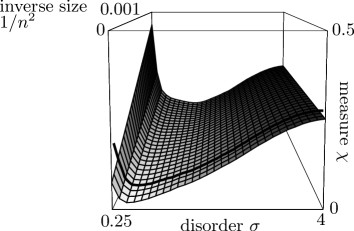
Figure 4: Numerical results for the measure $\chi$ with respect to the amount of disorder $\sigma$ and the inverse layer size $1/n^{2}$. An absolute minimum $\chi_{\text{min}}\approx 0.02$ is found at $\sigma\approx 0.5$ in the limit of $n\rightarrow\infty$. Note that only $10\%$ of the whole area is extrapolated (the area in front of the thick line).

This ratio turns out to be a monotonously increasing function in $t$, which is not surprising, since lower order terms in Eq. (7) are expected to dominate at shorter times. Thus, no visible deviation from the (diffusive) second order description arises, as long as the decay is “over”, before $L(t)$ reaches some value on the order of a fraction of one. Since the decay time scale is given by $\tau_{R}$, we are interested in $L(W,\tau_{R})$. If $L(\tau_{R})$ is on the order of one, the dynamics of the corresponding density wave in the corresponding model must exhibit significant deviations from diffusive, exponential decay. Because (apart from the model parameters $n$, $\sigma$) $\tau_{R}$ only depends on $W$ [cf. Eq. (11)], we may now, exploiting Eq. (15), reformulate $L(W,\tau_{R})$ only as a function of $W$ and the model parameters $n$, $\sigma$ but without any explicit dependence on $\beta$, $q$:

$$L[\,W,\tau_{R}(W)\,]\equiv R(W)$$ (16)

We call the above reformulation $R(W)$. It turns out that $R(W)$ decreases monotonously with $W$ such that the minimum $W$ for which $R(W)<1$ holds may be found from $R(W_{\text{min}})=1$. This $W_{\text{min}}$ corresponds to the maximum wavelength beyond which no diffusive behavior can be expected. Due to the fact that $\tilde{\Gamma}_{4}(t)$, $\tilde{\Gamma}_{2}(t)$ and $\tau_{R}(W)$, $\tau_{C}$ are numerically accessible, $W_{\text{min}}$, $W_{\text{max}}$ can be computed for a wide range of model parameters $n$, $\sigma$. In Fig. 4 we display the ratio $\chi\equiv W_{\text{min}}/W_{\text{max}}$ as a function of those model parameters. With the approximation $W\approx\beta^{2}\,q^{2}$ this ratio allows for the following interpretation:

$$\chi=\frac{W_{\text{min}}}{W_{\text{max}}}\approx\frac{q^{2}_{\text{min}}}{q^{2}_{\text{max}}}=\frac{l_{\text{min}}^{2}}{l_{\text{max}}^{2}}$$ (17)

Hence $\sqrt{\chi}$ (which no longer depends on $\beta$) may be viewed as the ratio of the shortest to the longest diffusive wavelength, the smaller it is, the larger is the diffusive regime.

Obviously, for each layer size $n$ there is some disorder that “optimizes” the diffusive regime (minimizes $\chi$). But, however, for $n=30$ (back of Fig. 4) we find $\sqrt{\chi_{\text{min}}}\approx 1/3$ at this optimum disorder, which indicates about one diffusive wavelength. Exactly those respective wavelengths have been chosen for the examples in Fig. 2 and the inset in Fig. 3, but not in Fig. 3 itself. For all $\sigma$ and up to $n=100$ (which is about the limit for our simple numerics) $\chi$ clearly appears to be of the form $\chi(\sigma,n)=A(\sigma)/n^{2}+B(\sigma)$. Extrapolating this $1/n^{2}$-behavior yields a suggestion for the infinite model $n=\infty$ (front of Fig. 4). According to this suggestion, we find $\sqrt{\chi_{\text{min}}}\approx 1/7$, again at optimum disorder. This indicates a rather small regime of diffusive wavelengths, even for the infinite system. We would like to repeat that these findings apply at infinite temperature, i.e., the above small diffusive regime is characterized by the fact that the dynamics within it are diffusive at all energies.

References

- [1] P. W. Anderson, Phys. Rev. 109 (1958) 1492.
- [2] R. Abou-Chacra, D. J. Thouless, P. W. Anderson, J. Phys. C 6 (1973) 1734.
- [3] P. A. Lee, T. V. Ramakrishnan, Rev. Mod. Phys. 57 (1985) 287.
- [4] B. Kramer, A. MacKinnon, Rep. Progr. Phys. 56 (1993) 1469.
- [5] L. Erdős, M. Salmhofer, H.-T. Yau, Annales Henri Poincare 8 (2007) 621.
- [6] T. Schwartz, G. Bartal, S. Fishman, M. Segev, Nature 446 (2007) 52.
- [7] A. Lherbier, B. Biel, Y.-M. Niquet, S. Roche, Phys. Rev. Lett. 100 (2008) 036803.
- [8] H.-P. Breuer, and F. Petruccione, The Theory of Open Quantum Systems, Oxford University Press, Oxford, 2007.
- [9] R. Steinigeweg, H.-P. Breuer, J. Gemmer, Phys. Rev. Lett. 99 (2007) 150601.
- [10] M. Michel, R. Steinigeweg, H. Weimer, Eur. Phys. J. Special Topics 151 (2007) 13.
- [11] R. Steinigeweg, J. Gemmer, M. Michel, Europhys. Lett. 75 (2006) 406.
- [12] M. Michel, J. Gemmer, G. Mahler, Int. J. Mod. Phys. B 20 (2006) 4855.
- [13] R. Steinigeweg, H.-J. Schmidt, Comp. Phys. Comm. 174 (2006) 853.
- [14] C. Bartsch, R. Steinigeweg, J. Gemmer, Phys. Rev. E 77 (2008) 011119.