Geometric Characteristics of Dynamic Correlations for Combinatorial Regulation in Gene Expression Noise

Abstract

Knowing which mode of combinatorial regulation (typically, AND or OR logic operation) that a gene employs is important for determining its function in regulatory networks. Here, we introduce a dynamic cross-correlation function between the output of a gene and its upstream regulator concentrations for signatures of combinatorial regulation in gene expression noise. We find that the correlation function is always upwards convex for the AND operation whereas downwards convex for the OR operation, whichever sources of noise (intrinsic or extrinsic or both). In turn, this fact implies a means for inferring regulatory synergies from available experimental data. The extensions and applications are discussed.

Cells live in a complex environment and continuously have to make decisions for different signals that they sense. A challenge in systems biology is to understand how signals are integrated. As the central information-processing units of living cells, transcription regulatory networks allow them to integrate different signals and generate specific responses of genes. The elementary computations are performed at the cis-regulatory regions of the genes: the transcription rate of each gene (the output) is a function of the active concentrations of each of the input transcription factors (TFs) AlonBook . Such a quantitative mapping between the regulator concentrations and the output of the regulated gene is known as the cis-regulatory input function (CRIF), which can be functioned as implementations of Boolean logic Glass73 ; Arkin94 in analogy to Boolean calculations that basic electronic devices perform Margolin05 . For example, two activators regulate a gene with AND or OR logic operation (refer Fig. 1). The notion of logic operations can also be generalized by introducing a continuous function that encodes the dependence of the rate of transcription on the concentrations of inputs AlonBook . Knowing which mode of combinatorial regulation that a gene employs is important for determining its function in regulatory networks. For example, the cis-regulatory module drives cellular patterns differently depending on how the gene integrates intracellular and extracellular signals at its regulatory region by endogenous and exogenous TFs Yuh98 ; Zhang09 .

Experiments performed on single cells have revealed that because TFs are often present in low copy numbers, stochastic fluctuations or noise in the concentrations of these molecules can have significant influences on gene regulation Elowitz02 ; Blake03 ; Kaern05 ; Zhou05 . The traditional fluctuation-dissipation relation derived by the linear noise approach Kapmen92 based on the mater equation gives the information only about the second-order moments. Recently, a modified fluctuation-dissipation relation was derived by Warmflash and Dinner Warmflash08 , which relates some third-order moments evaluated at the system steady state to the derivatives of a CRIF. Such a static cross correlation provides the information only about how three time series are correlated at the zero correlation time. From viewpoints of gene regulation, however, the binding of TFs to the DNA is context dependent, active in some genetic states but not in others. In particular, stochastic fluctuations, or ‘noise’, in gene expression propagate from active inputs to the outputs of regulated genes during signal integration. Thus, dynamic cross correlations Arkin97 ; Dunlop08 would provide a noninvasive means to probe modes of combinatorial regulation in gene expression noise. The purpose of this Letter is to demonstrate its potentials in detecting signatures of combinatorial interaction. Regarding the study of combinatorial regulation, there are other works Creighton03 ; Chen07 ; Pilpel01 ; Tsai05 ; Gertz09 . Usually, these papers used some real time-course microarray data to test their algorithms and identify some synergistic TFs.

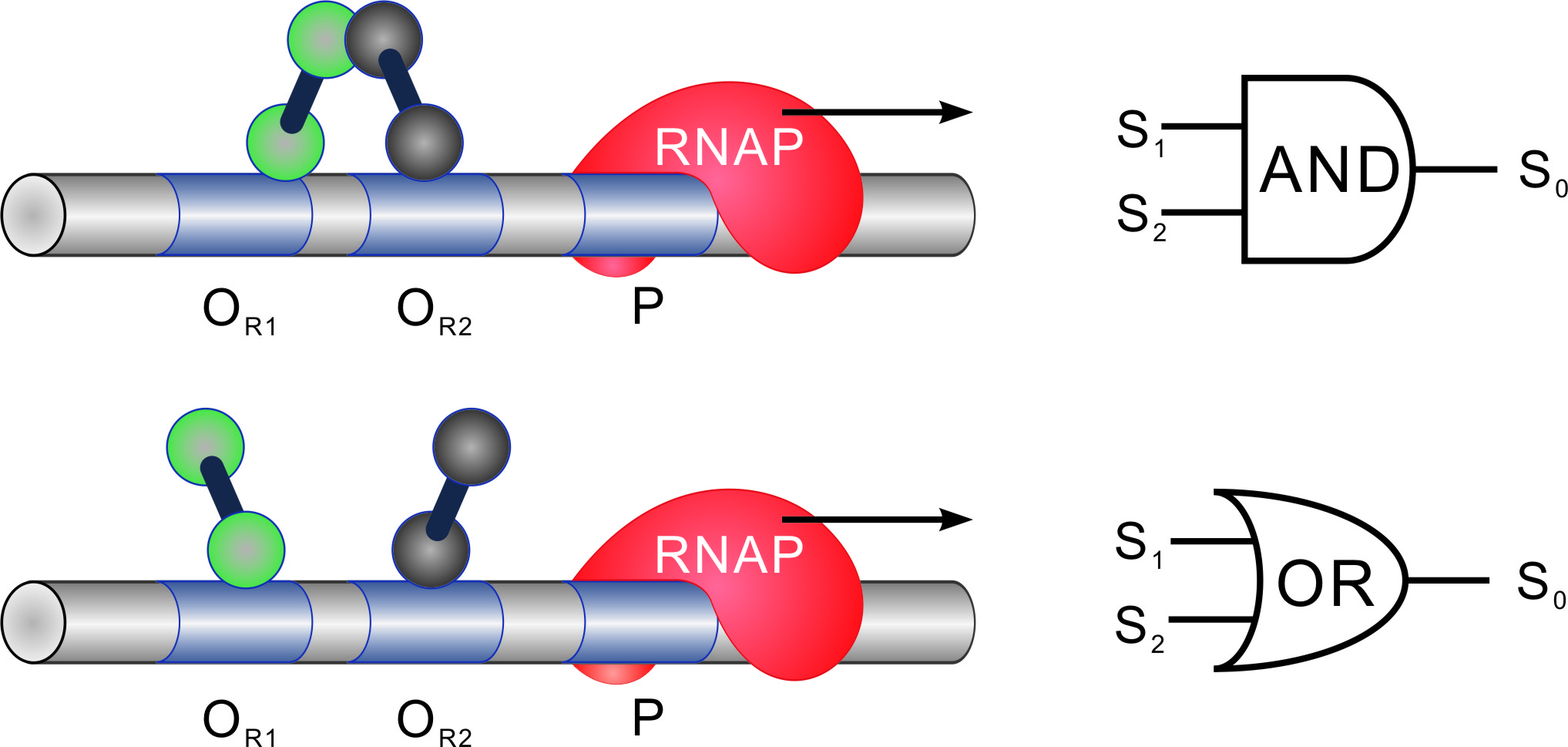
Figure 1: (color). Schematic illustration of cis-regulatory constructs. The regulatory functions are realized through the regulated recruitment of transcription factors and RNA polymerase (RNAP).

Before presenting our analysis, let us examine a real biological example. Consider a genetic circuit based on the phage-$\lambda$ operon Warmflash08 ; Joung94 . The corresponding biochemical reactions are listed in the Supporting Material supp , wherein how intrinsic and extrinsic noise sources generate are explained. We first perform realistic stochastic simulations of the whole circuit by using biologically reasonable parameter values and obtain three time series data of input TFs $S_{1}(t)$ and $S_{2}(t)$ and the output $S_{0}(t)$ Gillespie76 . We expect these simulations to faithfully reflect the biological system because the phage-$\lambda$ is a well-studied system for which many parameters are measured and comparable models are capable of accurately reproducing distributions of protein concentrations in prokaryotic systems Guido06 ; Mettetal06 . Then, according to Ref. supp , we calculate dynamic cross-correlation functions $R_{s_{1}s_{2},s_{0}}(\tau)$ for AND and OR operations, respectively. Figure 2 shows the dependence of the normalized dynamic cross-correlation function $R(\tau)$ on the correlation time $\tau$. Apparently, the correlation curve near the peak point close to the zero correlation time is upwards convex for AND operation and downwards convex for OR operation, whichever the sources of noise (intrinsic or extrinsic noise).

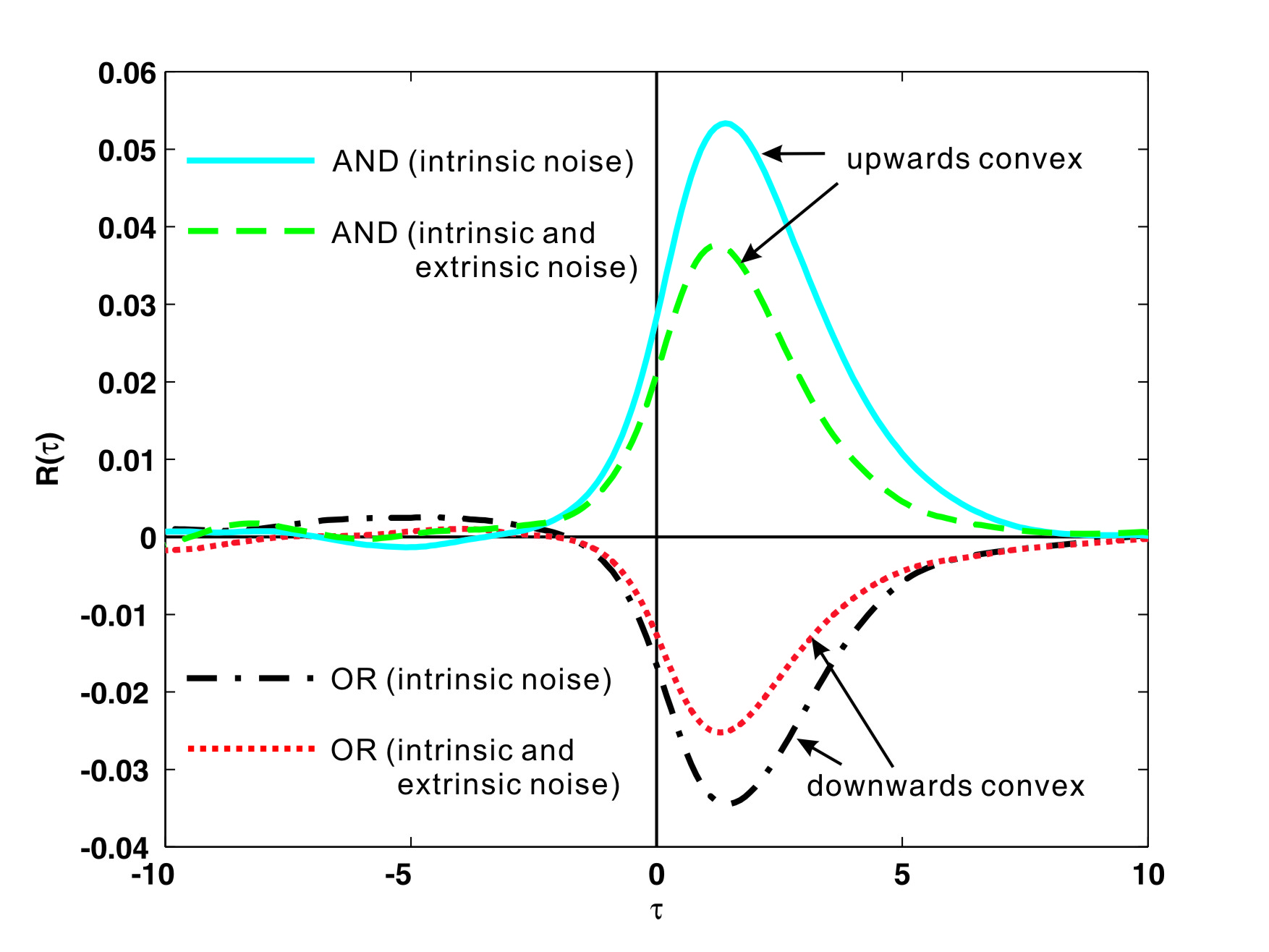
Figure 2: (color). Geometric characteristics of dynamic cross correlations for the phage-$\lambda$ operon, where $10^{3}$ cells are measured. There is an anti-correlation relationship between the convexity of dynamic cross-correlation curves for AND and OR operations.

Such an anti-correlation relationship between the convexity of dynamic cross-correlation functions for AND and OR operations is not a casual finding but is a general fact. In what follows, we will analytically verify this point using a simple yet general model as schematized in Fig. 1. The corresponding biochemical processes are modeled with the production and degradation of the TFs and the output only

$$\varnothing\overset{\alpha_{1}}{\longrightarrow}{\bf S}_{1}\overset{\beta_{1}}{\longrightarrow}\varnothing$$

$$\varnothing\overset{\alpha_{2}}{\longrightarrow}{\bf S}_{2}\overset{\beta_{2}}{\longrightarrow}\varnothing$$ (1)

$$\varnothing\overset{{\rm CRIF}(S_{1},S_{2})}{\longrightarrow}{\bf S}_{0}\overset{\beta_{0}}{\longrightarrow}\varnothing,$$

where $\rm S_{1}$ and $\rm S_{2}$, both of which are activators, represent the TF inputs to cis-regulatory module, $\rm S_{0}$ is the measured output of the regulated gene, and arrows from and to $\varnothing$ denote synthesis and degradation, respectively. The production rate of $\rm S_{0}$ is determined by the concentrations of the TFs and is encoded in the (dimensionless) cis-regulatory input function ${\rm CRIF}(S_{1},S_{2})$ (see Ref. supp for its analytic form).

Note that the accurate modeling of the system (1) should adopt the master equation Kapmen92 , but to show our analytic results, we instead take the following simplified Langevin equations

$$\frac{dS_{1}}{dt} = \alpha_{1}+E+I_{1}-\beta_{1}S_{1}$$

$$\frac{dS_{2}}{dt} = \alpha_{2}+E+I_{2}-\beta_{2}S_{2}$$ (2)

$$\frac{dS_{0}}{dt} = {\rm CRIF}(S_{1},S_{2})+E+I_{0}-\beta_{0}S_{0}.$$

Such an approximation can still describe well the motion of individual species molecules under some ideal conditions (see Ref. supp for interpretations). The above equations include terms for protein production rate $(\alpha_{i},\,i=0,1,2)$, protein degradation and dilution rate $(\beta_{i},\,i=0,1,2)$, and the contributions of intrinsic and extrinsic noise sources ($I_{i}\,(i=0,1,2)$ and $E$ respectively). Here, the extrinsic noise $E$ is defined as a stochastic fluctuation to globally measured components, whereas the intrinsic noise is assumed as stochastic fluctuations in the gene expression. Noise sources are modeled using Ornstein-Uhlenbeck processes by

$$\begin{split}\frac{dE}{dt}&=-\beta_{E}E+\sigma_{E}\eta_{E}\\ \frac{dI_{i}}{dt}&=-\kappa_{i}I_{i}+\sigma_{i}\eta_{i}\,\,\,(i=0,1,2).\end{split}$$ (3)

Assume that the white noise terms $\eta_{E}$, $\eta_{1}$, $\eta_{2}$ and $\eta_{0}$ are independent, identically distributed processes with the zero mean and the unit standard deviation. The parameters $\beta_{i}$ and $\kappa_{i}$ define the time scale of the noise, while $\sigma_{E}$ and $\sigma_{i}\,(i=0,1,2)$ set the standard deviation.

We expect perturbations due to noise to be so small that it might be valid to approximate our system using the second-order Taylor expansion of CRIF at the origin system. Denote $S_{i}^{eq}=\alpha_{i}/\beta_{i}\,\,(i=1,2)$. Define $s_{i}=S_{i}-S_{i}^{eq}\,(i=0,1,2)$, where $\displaystyle S_{0}^{eq}={\rm CRIF}(S_{1}^{eq},S_{2}^{eq})+a_{0}$ with $\displaystyle a_{0}=\frac{g_{11}}{2}\langle\langle s_{1}^{2}\rangle\rangle_{t}+g_{12}\langle\langle s_{1}s_{2}\rangle\rangle_{t}+\frac{g_{22}}{2}\langle\langle s_{2}^{2}\rangle\rangle_{t}$ in which the outside bracket represents the average over the time $t$, and $g_{11}$, $g_{12}$, $g_{22}$ are 2-order derivatives of the function CRIF with respect to variables $S_{1}$ and $S_{2}$, evaluated at the point $(S_{1}^{eq},S_{2}^{eq})$. This will result in the following equations

$$\frac{ds_{1}}{dt} = E+I_{1}-\beta_{1}s_{1}$$

$$\frac{ds_{2}}{dt} = E+I_{2}-\beta_{2}s_{2}$$ (4)

$$\frac{ds_{0}}{dt} = E+I_{0}-\beta_{0}s_{0}+g_{1}s_{1}+g_{2}s_{2}$$

$$+\frac{g_{11}}{2}s_{1}^{2}+g_{12}s_{1}s_{2}+\frac{g_{22}}{2}s_{2}^{2}-a_{0}.$$

For simplicity, we assume $\beta=\beta_{i}$ and $\kappa=\kappa_{i}\,(i=0,1,2)$, and without loss of generality, also assume $\beta\neq\kappa$, $\beta\neq 2\kappa$ in the following analysis. By calculation, we find $a_{0}=(g_{11}+2g_{12}+g_{22})\sigma_{E}^{2}/(8\beta^{3})+(g_{11}\sigma_{2}^{2}+g_{22}\sigma_{2}^{2})/(4\beta\kappa(\beta+\kappa))$.

Finally, define the dynamic cross correlation between $s_{0}(t)$ and $s_{1}(t)$, $s_{2}(t)$ as

$$R_{s_{1}s_{2},s_{0}}(\tau) = \langle\langle s_{1}(t)s_{2}(t)s_{0}(t+\tau)\rangle\rangle_{t},$$ (5)

where $\tau$ represents the correlation time. In simulations, this function is normalized to $R(\tau)=R_{s_{1}s_{2},s_{0}}(\tau)/\sqrt{R_{s_{1}s_{2},s_{1}s_{2}}(0)R_{s_{0},s_{0}}(0)}$. By complex calculations, we obtain the analytic expression of the unnormalized dynamic cross-correlation function supp , denoted by $R_{{\rm int}}(\tau)$,

$$R_{{\rm int}}(\tau)=\frac{g_{12}\sigma_{1}^{2}\sigma_{2}^{2}}{4\kappa^{2}(\beta^{2}-4\kappa^{2})^{2}}\left\{\begin{aligned} &\gamma e^{-\beta\tau}-\frac{\kappa^{2}}{\beta^{3}}e^{-2\beta\tau}+\frac{1}{\beta-2\kappa}e^{-2\kappa\tau}+\frac{2}{\beta}e^{-2(\beta+\kappa)\tau}\hskip 14.22636pt(\tau\geq 0)\\ &\frac{\kappa^{2}}{3\beta^{3}}e^{2\beta\tau}+\frac{1}{\beta+2\kappa}e^{2\kappa\tau}-\frac{2\kappa}{\beta(2\beta+\kappa)}e^{2(\beta+\kappa)\tau}\hskip 29.87547pt(\tau\leq 0)\end{aligned}\right.$$ (6)

in the presence of intrinsic noise only, where $\gamma=-\frac{4(\beta+\kappa)(\beta-\kappa)^{2}(3\beta^{2}+12\beta\kappa+4\kappa^{2})}{3\beta^{3}(2\beta+\kappa)(\beta^{2}-4\kappa^{2})}$. Note that the sign of $g_{12}$ is opposite for the AND and OR

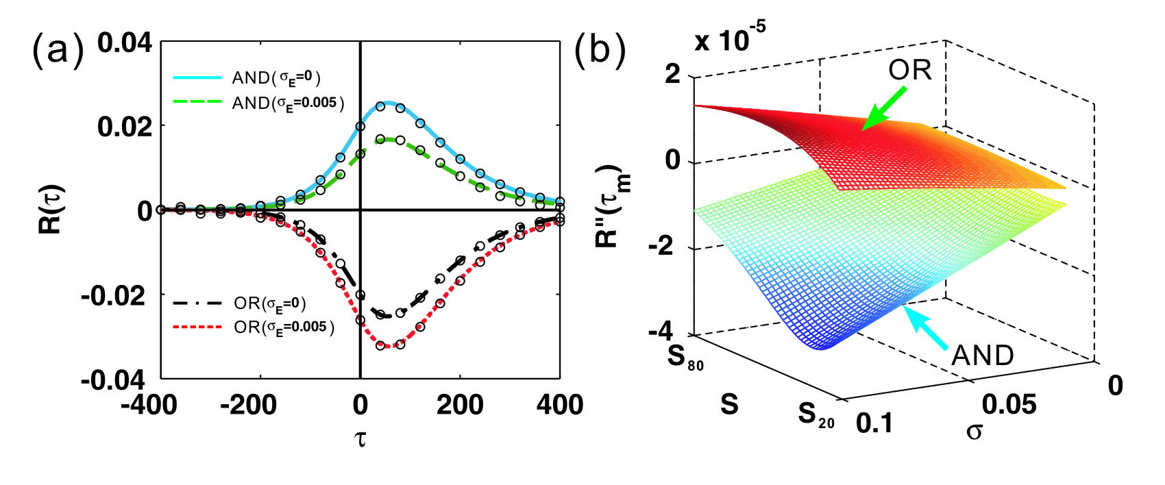
Figure 3: (color). Description of dynamic cross correlations in the modeled system. (a) The geometric characteristics of $R(\tau)$, where $K=100{\rm nM}$, $n=2$, $\alpha_{1}=\alpha_{2}=1{\rm molecule}/{\rm cell}/{\rm min}$, $\alpha_{0}=4{\rm molecules}/{\rm cell}/{\rm min}$ (a parameter in the CRIF function. See Ref. supp ), $\beta=0.01/{\rm min}$, $\kappa=0.02/{\rm min}$, $\sigma_{1}=\sigma_{2}=\sigma_{0}=0.02{(\rm molecules/cell)^{1/2}/min}$. The empty circles represent simulated results whereas the symbols indicated in the figure represent theoretical results; (b) The dependence of the 2-order derivative of the correlation function $R(\tau)$ at the peak point $\tau_{m}$, $R^{\prime\prime}(\tau_{m})$, on the noise intensity $\sigma$ and the signal concentration $S$, where $\sigma_{1}=\sigma_{2}=\sigma$, $\sigma_{0}=\sigma/10$, $S_{1}=S_{2}=S$ and the other parameters are similar to those in (a). $S_{20}$ and $S_{80}$ represent 20% and 80% maximal values of the input signal concentrations, respectively.

operations (see Ref. supp ). The simple analysis shows that $R_{{\rm int}}(\tau)$ has one peak at some small $\tau_{m}>0$. In particular, the convexity of $R_{{\rm int}}(\tau)$ at a small interval of $\tau_{m}>0$ but close to $\tau=0$ is anti-correlative for the two logic operations, referring Fig. 3(a).

In the simultaneous presence of extrinsic and intrinsic noise, the total unnormalized cross-correlation function can be expressed in the form of $R(\tau)=R_{{\rm int}}(\tau)+R_{{\rm ext}}(\tau)+R_{{\rm mix}}(\tau)$, where $R_{{\rm ext}}(\tau)$ represents the dynamic cross correlation in the case of extrinsic noise only and $R_{{\rm mix}}(\tau)$ represents the cross terms due to the cooperative effect of intrinsic and extrinsic noise. The analytic expressions of $R_{{\rm ext}}(\tau)$ and $R_{{\rm mix}}(\tau)$ are put in Ref. supp . Figure 3(a) shows that the extrinsic noise does not influence the convexity of the correlation function $R(\tau)$ for both logic operations, where the theoretical results are in good accord with the numerical results. Note that there is a difference in the effect of extrinsic noise on the location of the dynamic cross-correlation curve between Figs. 2 and 3(a) in the case of OR operation. That is, extrinsic noise uplifts the dynamic cross-correlation curve in Fig. 2, but it moves down the dynamic cross-correlation curve in Fig. 3(a). This is possibly because for the modeled system, the additive noise of capturing the effect of external fluctuations does not depend on the state variables whereas for the real system, the extrinsic noise that appears actually in the relevant Langevin equation is dependent of the state variables Gillespie00 . Figure 3(b) further shows that the convexity of $R(\tau)$ is robust to noise in the active region of the two input signals (here, by the active region we mean that concentrations of the input signals are beyond 20% of their maximal values Goldbeter81 ). This is because the 2-order derivative of $R(\tau)$ evaluated at the peak point, denoted by $R^{\prime\prime}(\tau_{m})$, the sign of which describes the local convexity of $R(\tau)$, is always negative (i.e., upwards convex) for the AND operation whereas positive (i.e., downwards convex) for the OR operation in this active region.

In conclusion, we have shown that the dynamic cross-correlation functions for AND and OR operations in gene expression noise have apparently distinct geometric characteristics (convexity). Such a difference is qualitative, depending neither on specific models nor on the sources of noise, and hence the essential difference reflected by the modes of combinatorial regulation. Moreover, since the dynamic correlation function utilizes statistics of the naturally arising fluctuations in the copy number of the species, its geometric characteristics can in turn help us efficiently detect signatures of combinatorial regulation with available experimental data. This is useful because proximity in DNA binding is not sufficient to infer combinatorial interactions, and they cannot be readily probed by traditional methods (e.g., knockouts) or high-throughput expression assays (e.g., microarray data).

Since stochastic fluctuations, or noise, exist inherently in biochemical reactions, using noise rather than external interference means to mine bioinformation related to gene regulation provides a new research line. Regarding this aspect, there have been some works, e.g., Cox et al. used noise to characterize some genetic circuits Cox08 , Dunlop et al. used correlation in gene expression noise to reveal the activity states of regulatory links Dunlop08 , Warmflash and Dinner used static cross correlations to detect signatures of combinatorial regulation in intrinsic biological noise Warmflash08 . We utilized dynamic cross correlations based on the nature of noise correlation to identify the modes of combinatorial regulation in intrinsic or extrinsic noise or both. In contrast to Warmflash and Dinner’s approach, our approach would have some advantages since dynamic cross correlations can in general provide more information about gene-gene correlation in expression than static cross correlations.

The method of dynamic cross correlation can also be extended to other situations of logic operations (ANDN, ORN, NAND, NOR). For example, consider a system with two input TFs and the output of a gene. If both TFs are activators, this case has been studied in this paper; If both are repressors, our method can still show that the dynamic correlation function $R(\tau)$ is upwards convex for NOR whereas downwards convex for NAND; If one TF is activator and the other is repressor, the $R(\tau)$ is upwards convex for ANDN whereas downwards convex for ORN. In the cases of XOR and EQU, however, the approach will be invalid since the input TFs may be activator or repressor. Except for inferring synergies between regulators, the idea of dynamic correlation (e.g., 2-point dynamic cross correlations introduced in Ref. Dunlop08 ; Nolte08 ) can even be used to determine the direction and relationship of interactions between arbitrary two regulators, i.e., to determine who regulates whom and who activates/represses whom. The details will be discussed elsewhere. Finally, the approach of dynamic cross correlation can be applied to other biological networks, e.g., RNA logic devices Win08 , nucleic acid logic circuits Seelig06 , signaling protein logic modules Prehoda00 , to identify the types of logic operations.

This work was supported by the Natural Science Key Foundation of People’s Republic of China (No. 60736028).

See pages ,- of appendix

References

- (1) U. Alon, An introduction to systems biology: design principles of biological circuits (Chapman & Hall, Boca Raton, FL, 2007).
- (2) L. Glass and S. A. Kayffman, J. Theor. Biol. 39, 103 (1973).
- (3) A. Arkin and J. Ross, Biophys. J. 67, 560 (1994).
- (4) A. A. Margolin and M. N. Stojanovic, Nature Biotech. 11, 1374 (2005).
- (5) C. H. Yuh, H. Bolouri, and E. H. Davidson, Science 279, 1896 (1998).
- (6) J. J. Zhang, Z. J. Yuan, and T. S. Zhou, Phys. Rev. E 79, 041903 (2009).
- (7) M. B. Elowitz et al., Science 287, 1183 (2002).
- (8) W. J. Blake et al., Nature 422, 633 (2003).
- (9) M. Kaern et al., Nat. Rev. Genet. 6, 451 (2005).
- (10) T. S. Zhou, L. N. Chen, and K. Aihara, Phys. Rev. Lett. 95, 178103 (2005).
- (11) N. G. van Kapmen, Stochastic process in physics and chemistry (North-Holland, 1992).
- (12) A. Warmflash and A. R. Dinner, Proc. Natl. Acad. Sci. U.S.A. 105, 17262 (2008).
- (13) A. Arkin, P. Shen, and J. Ross, Science 277, 1275 (1997).
- (14) M. J. Dunlop et al., Nat. Genet. 40, 1493 (2008).
- (15) C. Creighton and S. Hanash, Bioinformatics 19, 79 (2003).
- (16) C. T. Chen, J. C. Wang, and B. A. Cohen, Am. J. Hum. Genet. 80, 692 (2007).
- (17) Y. Pilpel, P. Sudarsanam, and G. M. Church, Nat. Genet. 29, 153 (2001).
- (18) H. K. Tsai et al., Proc. Natl. Acad. Sci. U.S.A. 102, 13532 (2005).
- (19) J. Gertz, E. D. Siggia, and B. A. Cohen, Nature 457, 215 (2009).
- (20) J. K. Joung, D. M. Koepp, and D. Hochschild, Science 265, 1863 (1994).
- (21) Supporting material.
- (22) D. T. Gillespie, J. Comput. Phys. 22, 403 (1976).
- (23) N. J. Guido et al., Nature 439, 856 (2006).
- (24) J. T. Mettetal et al., Proc. Natl. Acad. Sci. U.S.A. 103, 7304 (2006).
- (25) D. T. Gillespie, J. Chem. Phys. 113, 297 (2000).
- (26) A. Goldbeter and D. E. Koshland, Proc. Natl. Acad. Sci. U.S.A. 78, 6840 (1981).
- (27) C. D. Cox et al., Proc. Natl. Acad. Sci. U.S.A. 105, 10809 (2008).
- (28) G. Nolte et al., Phys. Rev. Lett. 100, 234101 (2008).
- (29) M. N. Win and C. D. Smolke, Science 322, 456 (2008).
- (30) G. Seelig et al., Science 314, 1585 (2006).
- (31) K. E. Prehoda et al., Science 290, 801 (2000).