Data boundary fitting using a generalised least-squares method

Abstract

In many astronomical problems one often needs to determine the upper and/or lower boundary of a given data set. An automatic and objective approach consists in fitting the data using a generalised least-squares method, where the function to be minimized is defined to handle asymmetrically the data at both sides of the boundary. In order to minimise the cost function, a numerical approach, based on the popular downhill simplex method, is employed. The procedure is valid for any numerically computable function. Simple polynomials provide good boundaries in common situations. For data exhibiting a complex behaviour, the use of adaptive splines gives excellent results. Since the described method is sensitive to extreme data points, the simultaneous introduction of error weighting and the flexibility of allowing some points to fall outside of the fitted frontier, supplies the parameters that help to tune the boundary fitting depending on the nature of the considered problem. Two simple examples are presented, namely the estimation of spectra pseudo-continuum and the segregation of scattered data into ranges. The normalisation of the data ranges prior to the fitting computation typically reduces both the numerical errors and the number of iterations required during the iterative minimisation procedure.

1 Introduction

Astronomers usually face, in their daily work, the need of determining the boundary of some data sets. Common examples are the computation of frontiers segregating regions in diagrams (e.g. colour–colour plots), or the estimation of reasonable pseudo-continua of spectra. Using for illustration the latter example, several strategies are initially feasible in order to get an analytical determination of that boundary. One can, for example, fit a simple polynomial to the general trend of the considered spectrum, masking previously disturbing spectroscopic features, such as important emission lines or deep absorption characteristics. Since this fit traverses the data, it must be shifted upwards a reasonable amount in order to be placed on top of the spectrum. However, since there is no reason to expect the pseudo-continuum following exactly the same functional form as the polynomial fitted through the spectrum, that shift does not necessarily provides the expected answer. As an alternative, one can also force the polynomial to pass over some special data points, which are selected to guide (actually to force) the fit through the apparent upper envelope of the spectrum. With this last method the result can be too much dependent on the subjectively selected points. In any case, the technique requires the additional effort of determining those special points.

With the aim of obtaining an objective determination of the boundaries, an automatic approach, based on a generalisation of the popular least-squares method, is presented in this work. Section 2 describes the procedure in the general case. As an example, the boundary fitting using simple polynomials is included in this section. Considering that these simple polynomials are not always flexible enough, Section 3 presents the use of adaptive splines, a variation of the typical fit to splines that allows the determination of a boundary that smoothly adapts to the data in an iterative way. Section 4 shows two practical uses of this technique: the computation of spectra pseudo-continuum and the determination of data ranges. Since the scatter of the data due to the presence of data uncertainties tends to bias the boundary determinations, Section 5 analyses the problem and presents a modification of the method that allows to confront this situation. Finally Section 6 summarises the main conclusions. In addition, Appendix A discusses the inclusion of constraints in the fits, whilst Appendix B describes how the normalisation of the data ranges prior to the data fitting can help to reduce the impact of numerical errors in some circumstances.

The method described in this work has been implemented into the program BoundFit, a FORTRAN code written by the author and available (under the GNU General Public License, version 3) at the following URL
http://www.ucm.es/info/Astrof/software/boundfit
All the fits presented in this paper have been computed with this program.

2 A generalised least-squares method

2.1 Introducing the asymmetry

The basic idea behind the method that follows is to introduce, in the fitting procedure, an asymmetric role for the data at both sides of a given fit, so the points located outside relative to that fit pull stronger toward themselves than the points at the opposite side. This idea is graphically illustrated in Fig. 1. As it is going to be shown, the problem is numerically treatable. In order to use the data asymmetrically, it is necessary to start with some initial guess fit, that in practice can be obtained employing the traditional least-squares method (with a symmetric data treatment). Once this initial fit is available, it is straightforward to continue using the data asymmetrically and, in an iterative process, determine the sought boundary.

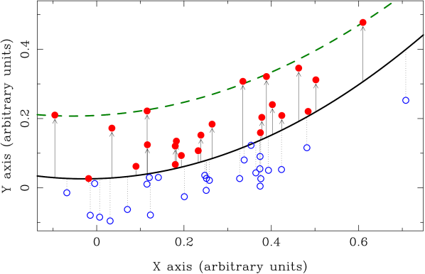
Figure 1: Graphical illustration of the asymmetrical weighting scheme described in Section 2.1 for the determination of the upper boundary of a particular data set. In this example a second-order polynomial is employed. The continuous thick line is the traditional (symmetric) ordinary least-squares fit for the whole set of data points, which is used as an initial guess for the boundary determination. The filled red circles are data points above that fit (i.e. outside), whereas the open blue circles are found below such frontier (inside). Filled circles receive the extra weighting factor parametrized by the asymmetry coefficient $\xi$ introduced in Eq. (3). Since this parameter is chosen to be $\xi>>1$, the minimisation process shifts the initial fit towards the upper region. By iterating the procedure, the final boundary fit, shown as the green dashed line, is obtained. The same method, but exchanging symbols weights, could be employed to determine the lower boundary limit (not shown).

Let’s consider the case of a two-dimensional data set consisting in $N$ points of coordinates $(x_{i},y_{i})$, where $x_{i}$ is an independent variable, and $y_{i}$ a dependent variable, which value has an associated and known uncertainty $\sigma_{i}$. An ordinary error-weighted least-squares fit is obtained by minimising the cost function $f$ (also called objective function in the literature concerning optimisation strategies), defined as

$$f(a_{0},a_{1},\ldots,a_{p})=\sum_{i=1}^{N}\left(\frac{y(x_{i})-y_{i}}{\sigma_{i}}\right)^{2},$$ (1)

where $y(x_{i})$ is the fitted function evaluated at $x=x_{i}$, and $a_{0},a_{1},\ldots,a_{p}$ are the unknown $(p+1)$ parameters that define such function. Actually, one should write the fitted function as $y(a_{0},a_{1},\ldots,a_{p};x)$.

In order to introduce the asymmetric weighting scheme, the cost function can be generalised introducing some new coefficients,

$$f(a_{0},a_{1},\ldots,a_{p})=\sum_{i=1}^{N}w_{i}|y(x_{i})-y_{i}|^{\alpha},$$ (2)

where $\alpha$ is now a variable exponent ($\alpha=2$ in normal least squares). For that reason the distance between the fitted function $y(x_{i})$ and the dependent variable $y_{i}$ is considered in absolute value. The new overall weighting factors $w_{i}$ are defined differently depending on whether one is fitting the upper or the lower boundary. More precisely

$$w_{i}\equiv\left\{\begin{array}[]{ll}\begin{array}[]{@{}c@{}}\textrm{upper}\\ \textrm{boundary}\end{array}&\left\{\begin{array}[]{ll}1/\sigma_{i}^{\beta}&\textrm{for}\;\;y(x_{i})\geq y_{i}\\ \xi/\sigma_{i}^{\beta}&\textrm{for}\;\;y(x_{i})<y_{i}\end{array}\right.\\ &\\ \begin{array}[]{@{}c@{}}\textrm{lower}\\ \textrm{boundary}\end{array}&\left\{\begin{array}[]{ll}\xi/\sigma_{i}^{\beta}&\textrm{for}\;\;y(x_{i})>y_{i}\\ 1/\sigma_{i}^{\beta}&\textrm{for}\;\;y(x_{i})\leq y_{i}\end{array}\right.\end{array}\right.$$ (3)

being $\beta$ the exponent that determines how error weighting is incorporated into the fit ($\beta=0$ to ignore errors, $\beta=2$ in normal error-weighted least squares), and $\xi$ is defined as an asymmetry coefficient. Obviously, for $\alpha=\beta=2$ and $\xi=1$, Eq. (2) simplifies to Eq. (1). As it is going to be shown later, the asymmetry coefficient must satisfy $\xi>>1$ for the method to provide the required boundary fit.

Leaving apart the particular weighting effect of the data uncertainties $\sigma_{i}$, the net outcome of introducing the factors $w_{i}$ is that the points that are classified as being outside from a given frontier simply have a higher weight that the points located at the inner side (see Fig. 1), and this difference scales with the particular value of the asymmetry coefficient $\xi$.

Thus, the boundary fitting problem reduces to finding the $(p+1)$ parameters $a_{0},a_{1},\ldots,a_{p}$ that minimise Eq. (2), subject to the weighting scheme defined in Eq. (3). In the next sections several examples are provided, in which the functional form of $y(x)$ is considered to be simple polynomials and splines.

2.2 Relevant issues

The method just described is, as defined, very sensitive to extreme data points. This fact, that at first sight may be seen as a serious problem, it is not necessarily so. For example, one may be interested in constraining the scatter exhibited by some measurements due to the presence error sources. In this case a good option would be to derive the upper and lower frontiers that surround the data, and in this scenario there is no need to employ an error-weighting scheme (i.e. $\beta=0$ would be the appropriate choice). On the other hand, there are situations in which the data sample contains some points that have larger uncertainties than others, and one wants those points to be ignored during the boundary estimation. Under this circumstance the role of the $\beta$ parameter in Eq. (3) is important. Given the relevance of all these issues concerning the impact of data uncertainties in the boundary computation, this topic is intentionally delayed until Section 5. At this point it is better to keep the problem in a more simplified version, which facilitates the examination of the basic properties of the proposed fitting procedure.

An interesting generalisation of the boundary fitting method described above consists in the incorporation of additional constraints during the minimisation procedure, like forcing the fit to pass through some predefined fixed points, or imposing the derivatives to have some useful values at particular points. A discussion about this topic has been included in Appendix A.

Another issue of great relevance is the appearance of numerical errors during the minimisation procedure. The use of data sets exhibiting values with different orders of magnitude, or with a very high number of data points, can be responsible for preventing numerical methods to provide the expected answers. In some cases a simple solution to these problems consists in normalising the data ranges prior to the numerical minimisation. A detailed description of this approach is presented in Appendix B.

2.3 Example: boundary fitting to simple polynomials

Returning to Eq. (2), let’s consider now the particular case in which the functional form of the fitted boundary $y(x)$ is assumed to be a simple polynomial of degree $p$, i.e.

$$y(x)=a_{0}+a_{1}x+a_{2}x^{2}+\ldots+a_{p}x^{p}.$$ (4)

In this case, the function to be minimized, $f(a_{0},a_{1},\ldots,a_{p})$, is also a simple function of the $(p+1)$ coefficients. In ordinary least squares one simply takes the partial derivatives of the cost function $f$ with respect to each of these coefficients, obtaining a set of $(p+1)$ equations with $(p+1)$ unknowns, which can be easily solved, as far as the number of independent points $N$ is large enough, i.e. $N\geq p+1$.

However, considering the special definition of the weighting coefficients $w_{i}$ given in Eq. (3), it is clear that in the general case an analytical solution cannot be derived without any kind of iterative approach, since during the computation of the considered boundary (either upper or lower), the classification of a particular data point as being inside or outside relative to a given fit explicitly depends on the function $y(x)$ that one is trying to derive. Fortunately numerical minimisation procedures can provide the sought answer in an easy way. For this purpose, the downhill simplex method (Nelder & Mead, 1965) is an excellent option. This numerical procedure performs the minimisation of a function in a multi-dimensional space. For this method to be applied, an initial guess for the solution must be available. This initial solution, together with a characteristic length-scale for each parameter to be fitted, is employed to define a simplex (i.e., a multi-dimensional analogue of a triangle) in the solution space. The algorithm works using only function evaluations (i.e. not requiring the computation of derivatives), and in each iteration the method improves the previously computed solution by modifying one of the vertices of the simplex. The simplex adapts itself to the local landscape, and contracts on to the final minimum. The numerical procedure is halted once a pre-fixed numerical precision in the sought coefficients is reached, or when the number of iterations exceeds a pre-defined maximum value $N_{\mbox{\scriptsize maxiter}}$. A well-known implementation of the downhill simplex method is provided by Press et al. (2002). For the particular case of minimising Eq. (2) while fitting a simple polynomial, a reasonable guess for the initial solution is supplied by the coefficients of an ordinary least-squares fit to a simple polynomial derived by minimising Eq. (1).

It is important to highlight that whatever the numerical method employed to perform the numerical minimisation, the considered cost function will probably exhibit a parameter-space landscape with many peaks and valleys. The finding of a solution is never a guarantee of having found the right answer, unless one has the resources to employ brute force to perform a really exhaustive search at sufficiently fine sampling of the cost function to find the global minimum. In situations where this problem can be serious, more robust methods, like those provided by genetic algorithms, must be considered (see e.g. Haupt & Haupt, 2004). Fortunately, for the particular problems treated in this paper, the simpler downhill method is a good alternative, considering that the ordinary least-squares method will likely give a good initial guess for the expected solution in most of the cases.

Figure 2: Panel (a): Example of upper boundary fitting using a 5th order polynomial. The initial data set correspond to 100 points randomly drawn from the function $y(x)=1/x$, assuming the uncertainty $\sigma=10$ for all the points in the $y$-axis. The dashed blue line is the ordinary least-squares fit to that data, used as the initial guess for the numerical determination of the boundary. Since all the points have the same uncertainty, there is no need for an error-weighted procedure. For that reason $\beta=0$ has been used in Eq. (3). In addition $\alpha=2$ and an asymmetry coefficient $\xi=1000$ were employed. The grey lines indicate the boundary fits obtained for $N_{\mbox{\scriptsize maxiter}}$ in the range from 5 to 2000 iterations, at arbitrary steps. The inset displays a zoomed plot region where some particular values of $N_{\mbox{\scriptsize maxiter}}$ are annotated over the corresponding fits. The continuous red line is the final boundary determination obtained using $N_{\mbox{\scriptsize maxiter}}=2000$. Panel (b): Effect of employing different asymmetry coefficients $\xi$ for the upper boundary fit shown in panel (a). In the four cases the same maximum number of iterations ($N_{\mbox{\scriptsize maxiter}}=2000$) has been employed, with $\alpha=2$. Panel (c): Effect of using different values of the power $\alpha$, with $N_{\mbox{\scriptsize maxiter}}=2000$ and $\xi=1000$. See discussion in Section 2.3.

For illustration, Fig. 2a displays an example of upper boundary fitting to a given data set, using a simple 5th order polynomial. As initial guess for the numerical minimisation, the ordinary least-squares fit for the data (shown with a dashed blue line) has been employed. The grey lines represent the corresponding boundary fits obtained using the downhill method previously described. Each line corresponds to a pre-defined maximum number of iterations $N_{\mbox{\scriptsize maxiter}}$ in downhill, as labelled over the lines in the plot inset. In this particular example the fitting procedure has been carried out without weighting with errors (i.e., assuming $\beta=0$), and using a power $\alpha=2$ and an asymmetry coefficient $\xi=1000$. It is clear that after a few iterations the intermediate fits move upwards from the initial guess (dashed blue line), until reaching the location marked with $N_{\mbox{\scriptsize maxiter}}=31$. Beyond this number of iterations, the fits move downwards slightly, rapidly converging into the final fit displayed with the continuous red line. Fig. 2b displays the effect of modifying the asymmetry coefficient $\xi$. The ordinary least-squares fit corresponds to $\xi=1$ (dashed blue line). The asymmetric fits are obtained for $\xi>1$. The figure illustrates how for $\xi=10$ and 100 the resulting upper boundaries do still leave points in the wrong side of the boundary. Only when $\xi=1000$ (continuous red line) is the boundary fit appropriate. Thus, a proper boundary fitting requires the asymmetry coefficient to be large enough to compensate for the pulling effect of the points that are in the inner side of the boundary. On the other hand, Fig. 2c shows the impact of changing the power $\alpha$ in Eq. (2). For the lowest value, $\alpha=1$ (dotted blue line), the fit is practically identical to the one obtained with $\alpha=2$ (continuous red line). For the largest values, $\alpha=3$ or 5 (dotted green and dashed orange lines), the boundaries are below the expected location, leaving some points outside (above) the fits. In these last cases the power $\alpha$ is too high and, for that reason, the distance from the boundary to the more distant points in the inner side have a too high effect in the cost function given by Eq. (2).

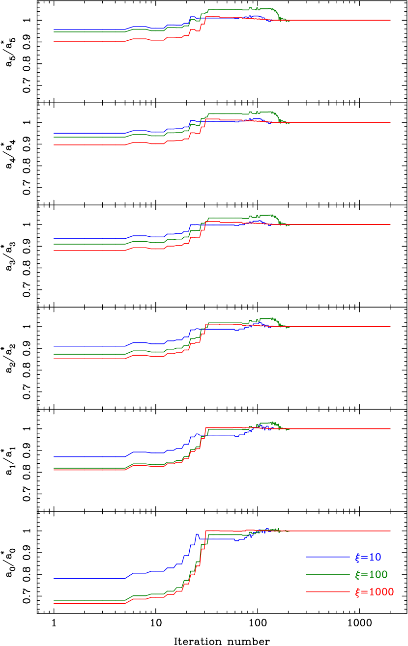
Figure 3: Variation in the fitted coefficients, as a function of the number of iterations, for the upper boundary fit (5th order polynomial $y(x)=\sum_{i=0}^{5}a_{i}\;x^{i}$) shown in Fig. 2a. Each panel represents the coefficient value at a given iteration ($a_{i}$, with $i=0,\ldots,5$, from bottom to top) divided by $a_{i}^{*}$, the final value derived after $N_{\mbox{\scriptsize maxiter}}=2000$ iterations. The same $y$-axis range is employed in all the plots. Red lines correspond to an asymmetry coefficient $\xi=1000$, whereas the blue and green grey lines indicate the coefficients obtained with $\xi=10$ and $\xi=100$, respectively (in all the cases $\alpha=2$ and $\beta=0$ have been employed). Note that the plot $x$-scale is in logarithmic units.

Another important aspect to take into account when using a numerical method is the convergence of the fitted coefficients. Fig. 3 displays, for the same example just described in Fig. 2b, the values of the 6 fitted polynomial coefficients as a function of the maximum number of iterations allowed. The figure includes the results for $\xi=10$, 100 and 1000 (using $\alpha=2$ and $\beta=0$ in the three cases). In overall, the convergence is reached faster when $\xi=1000$. Fig. 2a already showed that for this particular value of the asymmetry coefficient a quite reasonable fit is already achieved when $N_{\mbox{\scriptsize maxiter}}$=31. Beyond this maximum number of iterations the coefficients only change slightly, until they definitely settle around $N_{\mbox{\scriptsize maxiter}}\sim 140$.

Although simple polynomials can be excellent functional forms for a boundary determination (as shown in the previous example), when the data to be fitted exhibit rapidly changing values, a single polynomial is not always able to reproduce the observed trend. A powerful alternative in these situations consists in the use of splines. The next section presents an improved method that using classic cubic splines, but introducing additional degrees of freedom, offers a much larger flexibility for boundary fitting.

3 Adaptive Splines

3.1 Using splines with adaptable knot location

Splines are commonly employed for interpolation and modelling of arbitrary functions. Many times they are preferred to simple polynomials due to their flexibility. A spline is a piecewise polynomial function that is locally very simple, typically third-order polynomials (the so called cubic splines). These local polynomials are forced to pass through a prefixed number of points, $N_{\mbox{\scriptsize knots}}$, which we will refer as knots. In this way, the functional form of a fit to splines can be expressed as

$$\begin{array}[]{@{}r@{\;}l}y(x)=&s_{3}(k)[x-x_{\mbox{\scriptsize knot}}(k)]^{3}+s_{2}(k)[x-x_{\mbox{\scriptsize knot}}(k)]^{2}+\\ +&s_{1}(k)[x-x_{\mbox{\scriptsize knot}}(k)]+s_{0}(k),\end{array}$$

where ($x_{\mbox{\scriptsize knot}}(k),y_{\mbox{\scriptsize knot}}(k)$) are the $(x,y)$ coordinates of the $k^{\mbox{\scriptsize th}}$ knot, and $s_{0}(k)$, $s_{1}(k)$, $s_{2}(k)$, and $s_{3}(k)$ are the corresponding spline coefficients for $x\in[x_{\mbox{\scriptsize knot}}(k),x_{\mbox{\scriptsize knot}}(k+1)]$, with $k=1,\ldots,N_{\mbox{\scriptsize knots}}-1$. These coefficients are easily computable by imposing the set of splines to define a continuous function and that, in addition, not only the function, but also the first and second derivatives match at the knots (two additional conditions are required; typically they are provided by assuming the second derivatives at the two endpoints to be zero, leading to what are normally referred as natural splines). The computation of splines is widely described in the literature (see e.g. Gerald & Wheatley 1989).

The final result of a fit to splines will strongly depend on both, the number and the precise location of the knots. With the aim of having more flexibility in the fits, Cardiel (1999) explored the possibility of setting the location of the knots as free parameters, in order to determine the optimal coordinates of these knots that improve the overall fit of the data. The solution to the problem can be derived numerically using any minimisation algorithm, as the downhill simplex method previously described. In this way the set of splines smoothly adapts to the data. The same approach can be applied to the data boundary fitting, using as functional form for the function $y(x)$ in Eq. (2) the adaptive splines just described. It is important to highlight that in this case the optimal boundary fit requires not only to find the appropriate coefficients of the splines, but also the optimal location of the knots.

3.2 The fitting procedure

In order to carry out the double optimisation process (for the coefficients and the knots location) required to compute a boundary fit using adaptive splines, the following steps can be followed:

1. Fix the initial number of knots to be employed, $N_{\mbox{\scriptsize knots}}$. Using a large value provides more flexibility, although the number of parameters to be determined logically scales with this number, and the numerical optimisation demands a larger computational effort.

2. Obtain an initial solution with fixed knot locations. For this purpose it is sufficient, for example, to start by dividing the full $x$-range to be fitted by $(N_{\mbox{\scriptsize knots}}-1)$. This leads to a regular distribution of equidistant knots. The initial fit is then derived by minimising the cost function given in Eq. (2), leaving as free parameters the $y$-coordinates of all the knots simultaneously, while keeping fixed the corresponding $x$-coordinates. This numerical fit also requires a preliminary guess solution, than can be easily obtained through $(N_{\mbox{\scriptsize knots}}-1)$ independent ordinary least-squares fit of the data placed between each consecutive pair of knots, using for this purpose simple polynomials of degree 1 or 2. In this guess solution the $y$-coordinate for each knot is then evaluated as the average value for the two neighbouring preliminary polynomial fits (only one for the knots at the borders of the $x$-range). Obviously, if there is additional information concerning a more suitable knot arrangement than the equidistant pattern, it must be used to start the process with an even better initial solution which will facilitate a faster convergence to the final solution.

3. Refine the fit. Once some initial spline coefficients have been determined, the fit is refined by setting as free parameters the location of all the “inner” knots, both in the $x$- and $y$-directions. The outer knots (the first and last in the ordered sequence) are only allowed to be refined in the $y$-axis direction with the aim of preserving the initial $x$-range coverage. The simultaneous minimisation of the $x$ and $y$ coordinates of all the knots at once will imply finding the minimum of a multidimensional function with too many variables. This is normally something very difficult, with no guarantee of a fast convergence. The problem reveals to be treatable just by solving for the optimised coordinates of every single knot separately. In practice, a refinement can be defined as the process of refining the location of all the $N_{\mbox{\scriptsize knots}}$ knots, one at a time, where the order in which a given knot is optimised is randomly determined. Each knot optimisation requires, in turn, a value for the maximum number of iterations allowed $N_{\mbox{\scriptsize maxiter}}$. Thus, at the end of every single refinement process all the knots have been refined once. An extra penalisation can be introduced in the cost function with the idea of avoiding that knots exchange their order in the list of ordered sequence of knots. This inclusion typically implies that, if $N_{\mbox{\scriptsize knots}}$ is large, several knots end up colliding and having the same coordinates.The whole process can be repeated by indicating the total number of refinement processes, $N_{\mbox{\scriptsize refine}}$.

4. Optimise the number of knots. If after $N_{\mbox{\scriptsize refine}}$ refinement processes several knots have collided and exhibit the same coordinates, this is an evidence that $N_{\mbox{\scriptsize knots}}$ was probably too large. In this case, those colliding knots can be merged and the effective number of knots be accordingly reduced. If, on the contrary, the knots being used do not collide, it is interesting to check whether a higher $N_{\mbox{\scriptsize knots}}$ can be employed. With the new $N_{\mbox{\scriptsize knots}}$, step (iii) is repeated again.

Although at first sight it may seem excessive to use a large number of knots when some of them are going to end up colliding, these collisions will typically take place at optimised locations for the considered fit. As far as the minimisation algorithm is able to handle such large $N_{\mbox{\scriptsize knots}}$, it is not such a bad idea to start using an overestimated number and merge the colliding knots as the refinement processes take place.

The fitting algorithm can be halted once a satisfactory fit is found at the end of step (iii). By satisfactory one can accept a fit which coefficients do not significantly change by increasing neither $N_{\mbox{\scriptsize refine}}$ nor $N_{\mbox{\scriptsize maxiter}}$, and in which there are no colliding knots.

3.3 Example: boundary fitting to adaptive splines and comparison with simple polynomials

Figure 4: Example of the use of adaptive splines to compute the upper boundary of the same sample data displayed in Fig. 2. In this case $N_{\mbox{\scriptsize knots}}=15$ has been employed. Panel (a): the preliminary fit (dotted blue line) shows the initial guess determined from $(N_{\mbox{\scriptsize knots}}-1)$ independent ordinary least-squares fit of the data, as explained in Section 3.3. By imposing $N_{\mbox{\scriptsize maxiter}}=1000$ the fit improves, although in most cases the effective $N_{\mbox{\scriptsize maxiter}}$ is much lower since the algorithm computes spline coefficients that have converged before the number of iterations reaches that maximum value. The dashed green line shows the first fit obtained with still the knots at their initial equidistant locations. Successive refinements (light grey) allow the knots to change their positions, which leads to the final boundary determination (continuous red line, corresponding to $N_{\mbox{\scriptsize refine}}=40$). In all these fits $\xi=1000$, $\alpha=2$ and $\beta=0$ have been employed. Panel (b): Effect of using different asymmetry coefficients $\xi$ for the upper boundary fit shown in the previous panel. In the four cases $N_{\mbox{\scriptsize maxiter}}=1000$, $N_{\mbox{\scriptsize refine}}=40$, $\alpha=2$ and $\beta=0$ were used. Panel (c): Effect of employing different values of the power $\alpha$, with $\xi=1000$, $N_{\mbox{\scriptsize refine}}=40$ and $\beta=0$. See discussion in Section 3.3.

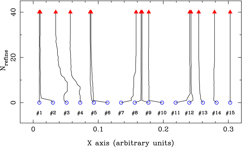
Figure 5: Variation in the location of the knots corresponding to the upper boundary fitting to adaptive splines displayed in Fig. 4a. Before introducing any refinement ($N_{\mbox{\scriptsize refine}}=0$), the 15 knots were regularly placed, as shown with the open blue circles. In each refinement process the inner knots are allowed to modify its location, one at a time. The first and last knots are fixed in order to preserve the fitted $x$-range. The final knot locations after $N_{\mbox{\scriptsize refine}}=40$ are shown with the filled red triangles.

To illustrate the flexibility of adaptive splines, Fig. 4a displays the corresponding upper boundary fit employing the same example data displayed in Fig. 2, for the case $N_{\mbox{\scriptsize knots}}=15$. The preliminary fit (shown as a dotted blue line) was computed by placing the $N_{\mbox{\scriptsize knots}}$ equidistantly spread in the $x$-axis range exhibited by the data, and performing $(N_{\mbox{\scriptsize knots}}-1)$ independent ordinary least-squares fit of the data placed between each consecutive pair of knots, using 2nd order polynomials, as explained in step (ii). Although unavoidably this preliminary fit is far from the final result (due to the fact that this is just the merging of several independent ordinary fits through data exhibiting large scatter and that the $x$-range between adjacent knots is not large), after $N_{\mbox{\scriptsize maxiter}}$ iterations without any refinement (i.e., without modifying the initial equidistant knot pattern) the algorithm provides the fit shown as the dashed green line. The light grey lines display the resulting fits obtained by allowing the knot locations to vary, and after 40 refinements one gets the boundary fit represented by the continuous red line. Since the knot location has a large influence in the quality of the boundary determination, very high values for $N_{\mbox{\scriptsize maxiter}}$ are not required (typically values for the number of iterations needed to obtain refined knot coordinates are $\sim 100$). Analogously to what was done with the simple polynomial fit, in Fig. 4b and 4c the effects of varying the asymmetry coefficient $\xi$ and the power $\alpha$ are also examined. In the case of $\xi$, it is again clear that the highest value ($\xi=1000$) leads to a tighter fit. Concerning the power $\alpha$, the best result is obtained when distances are considered quadratically, i.e. $\alpha=2$. For the largest values, $\alpha=3$ and 5, the resulting boundaries leave points above the fits. The case $\alpha=1$ is not very different to the quadratic fit, although in some regions (e.g. $x\in[0.01,0.04]$) the boundary is probably too high. In addition, Fig. 5 displays the variation in the location of the knots as $N_{\mbox{\scriptsize refine}}$ increases, for the final fit displayed in Fig. 4a. The initial equidistant pattern (open blue circles; corresponding to $N_{\mbox{\scriptsize refine}}=0$) is modified as each individual knot is allowed to change its coordinates. It is clear that some of the knots approximate and could be, in principle, merged into single knots, revealing that the initial number of knots was overestimated.

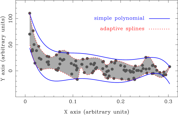
Figure 6: Comparison between different functional forms for the boundary fitting. The sample data set corresponds to the same values employed in Figs. 2 and 4. The boundaries have been determined using simple polynomials of 5th degree (continuous blue lines) and adaptive splines (dotted red lines; $N_{\mbox{\scriptsize knots}}=15$ and $N_{\mbox{\scriptsize refine}}=40$), following the steps given in Sections 2.3 and 3.3, respectively. The shaded area is simply the diagram region comprised between both adaptive splines boundaries. As expected, adaptive splines are more flexible, providing tighter boundaries than simple polynomials.

Finally Fig. 6 presents, for the same sample data employed in Figs. 2 and 4, the comparison between the boundary fits to simple polynomials (continuous blue lines) and to adaptive splines (dotted red lines). The shaded area corresponds to the diagram region comprised between the two adaptive splines boundaries. In this figure both the upper and the lower boundary limits, computed as described previously, are represented. It is clear from this graphical comparison that the larger number of degrees of freedom introduced with adaptive splines allows a much tighter boundary determination. The answer to the immediate question of which fit (simple polynomials or splines) is more appropriate will obviously depend on the nature of the considered problem.

4 Practical applications

4.1 Estimation of spectra pseudo-continuum

As mention in Section 1, a typical situation in which the computation of a boundary can be useful is in the estimation of spectra pseudo-continuum. The strengths of spectral features have been measured in different ways so far. However, although with slight differences among them, most authors have employed line-strength indices with definitions close to the classical expression for an equivalent width

$$\mbox{EW(\AA)}=\displaystyle\int_{\mbox{line}}(1-S(\lambda)/C(\lambda)\mbox{d}\lambda,$$ (5)

where $S(\lambda)$ is the observed spectrum and $C(\lambda)$ is the local continuum, usually obtained by interpolation of $S(\lambda)$ between two adjacent spectral regions (e.g. Faber, 1973; Faber et al., 1977; Whitford & Rich, 1983). In practice, as pointed out by Geisler (1984) (see also Rich, 1988), at low and intermediate spectral resolution the local continuum is unavoidably lost, and a pseudo-continuum is measured instead of a true continuum. The upper boundary fitting, either by using simple polynomials or adaptive splines, constitutes an excellent option for the estimation of that pseudo-continuum. To illustrate this statement, several examples are presented and discussed in this section. In all these examples, the boundary fits have been computed ignoring data uncertainties, i.e., assuming $\beta=0$ in Eq. (3). The impact of errors is this type of application is discussed later, in Section 5.

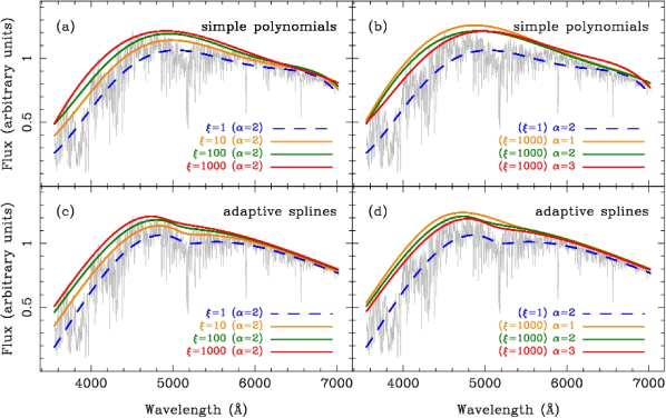
Figure 7: Examples of pseudo-continuum fits derived using upper boundaries with different tunable parameters. Panels (a) and (b) correspond to simple 5th order polynomials, whereas adaptive splines have been employed in panels (c) and  (d). The stellar spectrum corresponds to the K0V star HD003651 belonging to the MILES library (Sánchez-Blázquez et al., 2006). In the four panels the dashed blue line indicates the ordinary least-squares fit of the data. See discussion in Section 4.1.

Fig. 7 displays upper boundary fits for the particular stellar spectrum of HD003651 belonging to the MILES library (Sánchez-Blázquez et al., 2006). The results using simple polynomials and adaptive splines with different tunable parameters are shown. Panels 7a and 7b show the results derived using simple 5th-order polynomials, whereas panels 7c and 7d display the fits obtained employing adaptive splines with $N_{\mbox{\scriptsize knots}}=5$. The impact of modifying the asymmetry coefficient $\xi$ is explored in panels 7a and 7c (in these fits, $\alpha=2$ and $N_{\mbox{\scriptsize maxiter}}=1000$ have been used; the adaptive splines fits were refined $N_{\mbox{\scriptsize refine}}=10$ times). The dashed blue lines indicate the ordinary least-squares fits, i.e., those obtained when there is no effective asymmetry ($\xi=1$), which in each case was used as the initial guess fit in the numerical minimisation process. For relatively low values of the asymmetry coefficient ($\xi=10$ or 100) the fits are not as good as when using the largest value ($\xi=1000$). This is easy to understand, since the relatively large number of points to be fitted in this example ($N=3847$), requires that the points that still fall in the outer side of the boundary during the numerical minimisation of Eq. (2) overcome the pulling effect of the points in the inner side of the boundary. On the other hand, panels 7b and 7d display the effect of changing the power $\alpha$ in the fits. Again, the dashed blue lines correspond to the ordinary least-squares fits (in the rest of the cases $\xi=1000$ and $N_{\mbox{\scriptsize maxiter}}=1000$ have been used; the adaptive splines fits were refined $N_{\mbox{\scriptsize refine}}=10$ times). In these cases, the best boundary fits are obtained for $\alpha=1$, whereas for the larger values the fits depart from the expected result.

Figure 8: Examples of pseudo-continuum fits obtained using adaptive splines with different number of knots. The same stellar spectrum displayed in Fig. 7 is employed here. The dashed blue line indicates the ordinary least-squares fit of the data ($\xi=1$, $\alpha=2$). In the rest of the fits, $\xi=1000$, $\alpha=1$ and $N_{\mbox{\scriptsize refine}}=20$ have been used. The effect of using a different value of $N_{\mbox{\scriptsize knots}}$ is clearly visible. See discussion in Section 4.1.

The above example illustrates that the optimal asymmetry coefficient $\xi$ and power $\alpha$ during the boundary procedure can (and must) be tuned for the particular problem under study. Not surprisingly, this fact also concerns the number of knots when using adaptive splines. Fig. 8 shows the different results obtained when estimating the pseudo-continuum in the same stellar spectrum previously considered, employing different values of $N_{\mbox{\scriptsize knots}}$. As expected, the fit adapts to the irregularities exhibited by the spectrum as the number of knots increases. This is something that for some purposes may not be desired. For instance, the fits obtained with $N_{\mbox{\scriptsize knots}}=12$, and more notably with $N_{\mbox{\scriptsize knots}}=16$, detect the absorption around the Mg i feature at $\lambda\sim 5200$ Å, and for this reason these fits underestimate the total absorption produced at this wavelength region. In situations like this the boundary obtained with a lower number of knots may be more suitable. Obviously there is no general rule to define the right $N_{\mbox{\scriptsize knots}}$, since the most convenient value will depend on the nature of the problem under study.

Figure 9: Comparison of different strategies in the computation of the pseudo-continuum for the measurement of line-strength indices. The same stellar spectrum displayed in Fig. 7 is employed here. In this example three Balmer features are analised, namely H$\delta$, H$\gamma$ and H$\beta$ (from left to right), showing the commonly employed blue, central and red sidebands used in their measurement. Top panels correspond to the traditional method in stellar population studies, in which the pseudo-continuum is computed as the straight line joining the mean fluxes in the blue and red sidebands, respectively. In the middle panels the pseudo-continua have been computed as the straight line joining the values of the upper boundary fits (second order polynomials fitted to the three bandpasses; dotted lines), evaluated at the centres of the blue and red bandpasses. Finally, in the bottom panels the pseudo-continua are not computed as straight lines, but as the upper boundary fits themselves. In each case the resulting line-strength value (area comprised between the pseudo-continuum fit and the stellar spectrum) is shown. See discussion in Section 4.1.

In order to obtain a quantitative determination of the impact of using the upper boundary fit instead in the estimation of local pseudo-continuum, Fig. 9 compares the actual line-strength indices derived for three Balmer lines (H$\beta$, H$\gamma$ and H$\delta$, from right to left) using three different strategies. For this particular example the same stellar spectrum displayed in Fig. 7 has been used. Overplotted on each spectrum are the bandpasses typically used for the measurement of these spectroscopic features. In particular, de bandpasses limits for H$\beta$ are the revised values given by Trager (1997), whereas for H$\gamma$ and H$\delta$ the limits correspond to H$\gamma_{F}$ and H$\delta_{F}$, as defined by Worthey & Ottaviani (1997). For each feature, the corresponding line-strength has been computed by determining the pseudo-continuum using: i) the straight line joining the mean fluxes in the blue and red bandpasses (top panels) which is the traditional method; ii) the straight line joining the values of the upper boundary fits evaluated at the centres of the same bandpasses (central panels); and iii) the upper boundary fits themselves (bottom panels). For the cases ii) and iii) the upper boundary fits have been derived using a second order polynomial fitted to the three bandpasses. The resulting line-strength indices, numerically displayed above each spectrum, have been computed as the area comprised between the adopted pseudo-continuum fit and the stellar spectrum within the central bandpass. For the three Balmer lines it is clear that the use of the boundary fit provides larger indices. The traditional method provides very bad values for H$\gamma$ and H$\delta$ (which are even negative!), given that the pseudo-continuum is very seriously affected by the absorption features in the continuum bandpasses. This is a well-known problem that has led many authors to seek for alternative bandpass definitions (see e.g. Rose, 1994; Vazdekis & Arimoto, 1999) which, on the other hand, are not immune to other problems related to their sensitivity to spectral resolution and their high signal-to-noise requirements. These are very important issues that deserve a much careful analysis, that is beyond the aim of this paper, and they are going to be studied in a forthcoming work (Cardiel 2009, in preparation).

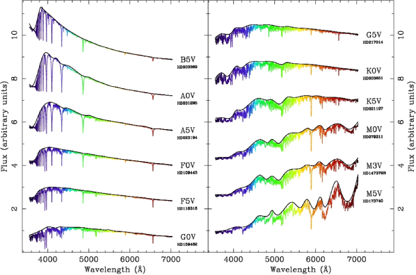
Figure 10: Examples of pseudo-continuum fits using adaptive splines. Several stars from the stellar library MILES (Sánchez-Blázquez et al., 2006), spanning different spectral types, have been selected. The fitted pseudo-continua (continuous black line) have been automatically determined employing $N_{\mbox{\scriptsize knots}}=19$, $N_{\mbox{\scriptsize maxiter}}=1000$, $N_{\mbox{\scriptsize refine}}=20$, $\xi=1000$, $\alpha=2$ and $\beta=0$.

The results of Fig. 7 reveal that, for the wavelength interval considered in that example, the boundary determinations obtained by using polynomials and adaptive splines are not very different. However, it is expected that as the wavelength range increases and the expected pseudo-continuum becomes more complex, the larger flexibility of adaptive splines in comparison with simple polynomials should provide better fits. To explore this flexibility in more detail, Fig. 10 shows the result of using adaptive splines to estimate the pseudo-continuum of 12 different spectra corresponding to stars exhibiting a wide range of spectral types (from B5V to M5V), selected from the empirical stellar library MILES (Sánchez-Blázquez et al., 2006) previously mentioned. Although in all the cases the fits have been computed blindly without considering the use of an initial knot arrangement appropriate for the particularities of each spectral type, it is clear from the figure that adaptive splines are flexible enough to give reasonable fits independently of the considered star. More refined fits can be obtained using an initial knot pattern more adjusted to the curvature of the pseudo-continuum exhibit by the stellar spectra.

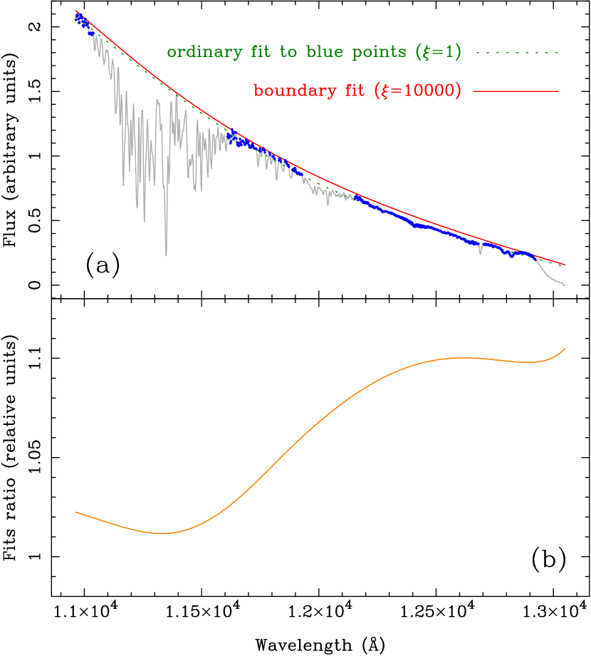
Figure 11: Comparison of the results of using an ordinary fit and adaptive splines when deriving the telluric correction in a particular spectroscopic calibration. Panel (a): the light grey line corresponds to the spectrum obtained in the J band of the hot star HD165174. Some special points of this spectrum have been manually selected (small blue points) to determine the approximate pseudo-continuum. The resulting ordinary fit to adaptive splines (i.e. adopting $\xi=1$) using exclusively these selected points is displayed with the dotted green line. A more suitable fit (continuous red line) is obtained employing $\xi=10000$, in which case the fit is performed over the whole spectrum. The two fits have been carried out with $N_{\mbox{\scriptsize knots}}=3$, $N_{\mbox{\scriptsize maxiter}}=1000$, $N_{\mbox{\scriptsize refine}}=10$, $\alpha=2$ and $\beta=0$. Panel (b): ratio between the two fits displayed in the previous panel.

A good estimation of spectra pseudo-continuum is very useful, for example, when correcting spectroscopic data from telluric absorptions using featureless (or almost featureless) calibration spectra. This is a common strategy when performing observations in the near-infrared windows. Fig. 11a illustrates a typical example, in which the observation of the hot star V986 Oph (HD165174, spectral type B0III) is employed to determine the correction. This star was observed in the J band as part of the calibration work of the observations presented in Cardiel et al. (2003). The stellar spectrum is shown in light grey, whereas the blue points indicate a manual selection of spectrum regions employed to estimate the overall pseudo-continuum. The dotted green line corresponds to the ordinary least-squares fit of these points, whereas the red continuous line is the upper boundary obtained with adaptive splines using $N_{\mbox{\scriptsize knots}}=3$ with an asymmetry coefficient $\xi=10000$. In Fig. 11b the ratio between both fits in represented, showing that there are differences up to a few percent between these fits. Two kind of errors are present here. In overall the ordinary least-squares fit underestimates the pseudo-continuum level, which introduces a systematic bias on the resulting depth of the telluric features (the whole curve displayed in Fig. 11b is above 1.0). In addition, since the selected blue points do include real (although small) spectroscopic features, there are variations as a function of wavelength of the above discrepancy. These differences can be important when trying to perform a high-quality spectrophotometric calibration. It is important to highlight that an important additional advantage of the boundary fitting is that this method does not require the masking of any region of the problem spectrum, which avoids the effort (and the subjectivity) of selecting special points to guide the fit.

Another important aspect concerning the use of boundary fits for the determination of the pseudo-continuum of spectra is that this method can provide an alternative approach for the estimation of the pseudo-continuum flux when measuring line-strength indices. Instead of using the average fluxes in bandpasses located nearby the (typically central) bandpass covering the relevant spectroscopic feature, the mean flux on the upper boundary can be employed. In this case it is important to take into account that flux uncertainties will bias the fits towards higher values. Under these situations the approach described later in Section 5 can be employed. Concerning this problem is worth mentioning here the method presented by Rogers et al. (2008), who employ a boosted median continuum to derive equivalent widths more robustly than using the classic side-band procedure.

4.2 Estimation of data ranges

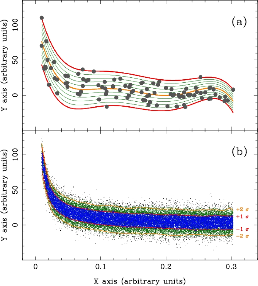
Figure 12: Examples of data boundary applications for the estimation of data ranges. Panel (a): Using the lower and upper boundary limits for the data displayed in Figs. 2, 4 and 6, and computed using simple 5th order polynomials, it is trivial to subdivide the range spanned by the data in the $y$-axis by creating a regular grid (i.e. contant $\Delta y$ at a fixed $x$) between both boundary limits. In this example the region has been subdivided in ten intervals. Panel (b): 30000 points randomly drawn from the functional form $y=1/x$, with $\sigma=10$ for all the points. Splitting the $x$-range in 100 intervals, sorting the data within each interval and keeping track of the subsets containing 68.27% ($\pm 1\sigma$; blue points) and 95.44% ($\pm 2\sigma$; green points) of the data points around the median, it is possible to compute the upper and lower boundaries for those two subsets (continuous red and orange lines, respectively). The boundaries in this example have been determined using adaptive splines with $N_{\mbox{\scriptsize knots}}=15$, $N_{\mbox{\scriptsize itermax}}=1000$, $N_{\mbox{\scriptsize refine}}=10$, $\alpha=2$, and $\beta=0$.

A quite trivial but useful application of the boundary fits is the empirical determination of data ranges. One can consider scenarios in which it is needed to subdivide the region spanned by the data in a particular grid. Fig. 12a illustrates this situation, making use of the 5th order polynomial boundaries corresponding to the data previously used in Figs. 2, 4, and 6. Once the lower and the upper boundaries are available, it is trivial to generate a grid of lines dividing the region comprised between the boundaries as needed.

A more complex scenario is that in which the data exhibit a clear scatter around some tendency, and one needs to determine regions including a given fraction of the points. A frequent case appears when one needs to remove outliers, and then it is necessary to obtain an estimation of the regions containing some relevant percentages of the data. In Fig. 12b this situation is exemplified with the use of a simulated data set consisting in 30000 points, for which the regions that include 68.27% and 95.44% of the centred data points, corresponding to $\pm 1\sigma$ and $\pm 2\sigma$ in a normal distribution, have been determined by first selecting those data subsets, and then fitting their corresponding boundaries using adaptive splines, as explained with more detail in the figure caption.

5 The impact of data uncertainties

Although the method described in Section 2 already takes into account data uncertainties through their inclusion as a weighting parameter (governed by the exponent $\beta$), it is important to highlight that this weighting scheme does not prevent the boundary fits to be highly biased due to the presence of such uncertainties. For example, in the determination of the pseudo-continuum of a given spectrum, even considering the same error bars for the fluxes at all wavelengths, the presence of noise unavoidably produces some scatter around the real data. When fitting the upper boundary to a noisy spectrum the fit will be dominated by the points that randomly exhibit the largest positive departures. Under these circumstances, two different alternatives can be devised:

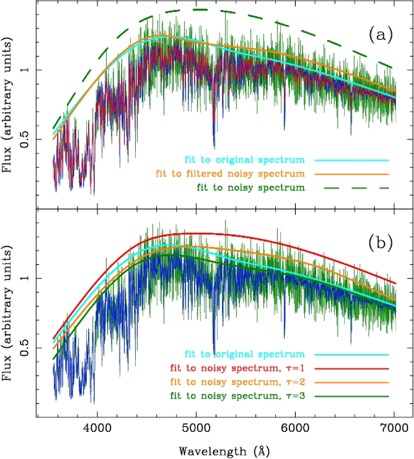
Figure 13: Comparison of the two approaches described in Section 5 for the boundary fitting with data uncertainties. Panel (a): original spectrum of HD003651 without noise (blue spectrum), spectrum with artificially added noise (green spectrum) and noisy spectrum after a Gaussian filtering (red spectrum). Note that the original (blue) and the filtered noisy (red) spectra are almost coincident. The upper boundary displayed with a dashed green line is the fit to the noisy spectrum using adaptive splines, whereas the upper boundaries plotted with continuous orange and cyan lines are the fits to the filtered noisy spectrum and to the original spectrum, respectively. Panel (b): original and noisy spectra are plotted with blue and green lines, respectively (the filtered spectrum is not plotted here). The cyan line is again the fit to the original spectrum. The rest of the boundary lines indicate the fits to the noisy spectrum using different values of the cut-off parameter (red $\tau=1$, orange $\tau=2$, and green $\tau=3$). In all the fits $N_{\mbox{\scriptsize knots}}=5$, $N_{\mbox{\scriptsize maxiter}}=1000$, $\xi=1000$, $\alpha=1$, $\beta=0$, and $N_{\mbox{\scriptsize refine}}=10$ have been employed. See discussion in Section 5.

1. To perform a previous rebinning or filtering of the data prior to the boundary fitting, in order to eliminate, or at least minimize, the impact of data uncertainties. After the filtering one assumes that these uncertainties are not seriously biasing the boundary fit. In this way one can employ the same technique described in Section 2. This approach is illustrated in Fig. 13a. In this case the original spectrum of HD00365 (also employed in Figs. 7 and 8), as extracted from the MILES library (Sánchez-Blázquez et al., 2006), is considered as a noise-free spectrum (plotted in blue). Its corresponding upper boundary fit using adaptive splines with $N_{\mbox{\scriptsize knots}}=5$ is shown as the cyan line. This original spectrum has been artificially degraded by considering an arbitrary signal-to-noise ratio per pixel S/N=10 (displayed in green), and the resulting upper boundary fit is shown with a dashed green line. It is obvious that this last fit is highly biased, being dominated by the points with higher fluxes. Finally, the noisy spectrum has been filtered by convolving it with a Gaussian kernel (of standard deviation 100 km/s), with the result being over-plotted in red. Note that this filtered spectrum overlaps almost exactly with the original spectrum. The boundary fit plotted with the continuous orange line is the upper boundary for that filtered spectrum. Although the result is not the same as the one derived with the original spectrum, it is much better than the one directly obtained over the noisy spectrum.

2. To allow a loose boundary fitting. Another possibility consists in trying to leave a fraction of the points with extreme values to fall outside (i.e., in the wrong side) of the boundary, specially those with higher uncertainties. This option is easy to parametrize by introducing a cut-off parameter $\tau$ into the overall weighting factors given in Eq. (3). The new factors can then be computed as

   $$w_{i}\equiv\left\{\begin{array}[]{ll}\begin{array}[]{@{}c@{}}\textrm{upper}\\ \textrm{boundary}\end{array}&\left\{\begin{array}[]{ll}1/\sigma_{i}^{\beta}&\textrm{for}\;\;y(x_{i})\geq y_{i}-\tau\sigma_{i}\\ \xi/\sigma_{i}^{\beta}&\textrm{for}\;\;y(x_{i})<y_{i}-\tau\sigma_{i}\end{array}\right.\\ &\\ \begin{array}[]{@{}c@{}}\textrm{lower}\\ \textrm{boundary}\end{array}&\left\{\begin{array}[]{ll}\xi/\sigma_{i}^{\beta}&\textrm{for}\;\;y(x_{i})>y_{i}+\tau\sigma_{i}\\ 1/\sigma_{i}^{\beta}&\textrm{for}\;\;y(x_{i})\leq y_{i}+\tau\sigma_{i}\end{array}\right.\end{array}\right.$$ (6)

   where $\sigma_{i}$ is the uncertainty associated to the dependent variable $y_{i}$. The cut-off parameter assigns to a point that falls outside of the boundary by distance that is less than or equal to $\tau\sigma_{i}$ the same low weight during the fitting procedure than the weight that receive the inner points. In other words, points like that do not receive the extra weighting factor provided by the asymmetry coefficient $\xi$, even though they are outside of the boundary. Note that $\tau=0$ simplifies the algorithm to the one described in Section 2. Fig. 13b illustrates the use of the cut-off parameter $\tau$ in the upper boundary fitting of the spectrum of HD003651. The cyan boundary is again the upper boundary determination using adaptive splines with the original spectrum. The rest of the boundary fits correspond to the use of the weighting scheme given in Eq. (6) for different values of $\tau$, as indicated in the legend. As $\tau$ increases, a larger number of points are left outside of the boundary during the minimisation procedure. In the example, the value $\tau=3$ seems to give a reasonable fit in the redder part of the spectrum, although in the bluer region the corresponding fit is too low. It is clear from this example that to define a correct value of $\tau$ is not a trivial issue. Most of the times the most suited $\tau$ will be a compromise between a high value (in order to avoid the bias introduced by highly deviant points) and a low value (in order to avoid leaving outside of the boundary right data points).

Figure 14: Study of the impact of variable signal-to-noise ratio in the upper boundary fitting of the spectrum of the star HD003651. In both panels the original spectrum (blue) is plotted together with the same spectrum after artificially adding noise (green) corresponding to a signal-to-noise ratio per pixel S/N=3 for $\lambda\leq 4200$ Å, and to S/N=50 for $\lambda>4200$ Å. The cyan line indicates the upper boundary fit to the original spectrum. Panel (a): In these fits the cut-off parameter has been ignored ($\tau=0$), but different values of the power $\beta$, as indicated in the legend, are employed. Note that the unweighted fit ($\beta=0$; dashed green line) is highly biased. Panel (b): the same fits of the previous panel are repeated here but using $\tau=2$. In all the fits $N_{\mbox{\scriptsize knots}}=5$, $N_{\mbox{\scriptsize maxiter}}=1000$, $\xi=1000$, $\alpha=1$, and $N_{\mbox{\scriptsize refine}}=10$ have been employed. See discussion in Section 5.

An additional complication arises when one combines in the same data set points with different uncertainties. It is in these situations when the role of the power $\beta$ in Eq. (2) becomes important. To illustrate the situation, Fig. 14 shows the different pseudo-continuum estimations obtained again for the star HD003651, but now considering that the spectrum is much noisier below 4200 Å than above this wavelength. In panel 14a the fits are derived ignoring the cut-off parameter previously discussed (i.e. assuming $\tau=0$), but with different values of $\beta$. In the unweighted case ($\beta=0$, dashed green line) the resulting upper boundary is dramatically biased for $\lambda<4200$ Å due to the presence of highly deviant fluxes. The use of non-null (and positive) values of $\beta$ induces the fit to be less dependent on the noisier values, being necessary a value as high as $\beta=3$ to obtain a fit similar to the one obtained in absence of noise (cyan line). However, since the fitted spectrum (green) do still have noise for $\lambda>4200$ Å, all the fits in that region are still biased compared to the fit for the original spectrum (cyan). In order to deal not only with the variable noise, but with the noise itself independently of its absolute value, it is possible to combine the effect of a tuned $\beta$ value with the introduction of a cut-off parameter $\tau$. Fig. 14b shows the results derived employing a fixed value $\tau=2$ with the same variable values of $\beta$ used in the previous panel. In this case, the boundary corresponding to $\beta=2$ (magenta) exhibits an excellent agreement with the fit for the original spectrum (cyan) at all wavelengths. Thus, the combined effect of an error-weighted fit and the use of a cut-off parameter is providing a reasonable boundary determination, even under the presence of wavelength dependent noise.

6 Conclusions

This work has confronted the problem of obtaining analytical expressions for the upper and lower boundaries of a given data set. The task reveals treatable using a generalised version of the very well-known ordinary least-squares fit method. The key ideas behind the proposed method can be summarised as follows:

• The sought boundary is iteratively determined starting from an initial guess fit. For the analysed cases an ordinary least-squares fit provides a suitable starting point. At every iteration in the procedure a particular fit is always available.

• In each iteration the data to be fitted are segregated in two subgroups depending on their position relative to the particular fit at that iteration. In this sense, points are classified as being inside or outside of the boundary.

• Points located outside of the boundary are given an extra weight in the cost function to be minimized. This weight is parametrized through the asymmetry coefficient $\xi$. The net effect of this coefficient is to generate a stronger pulling effect of the outer points over the fit, which in this way shifts towards the frontier delineated by the outer points as the iterations proceed.

• The distance from the points to a given fit are introduced in the cost function with a variable power $\alpha$, not necessarily in the traditional squared way. This supplies an additional parameter to play with when performing the boundary determination.

• Since data uncertainties are responsible for the existence of highly deviant points in the considered data sets, their incorporation in the boundary determination has been considered in two different and complementary ways. Errors can readily be incorporated into the cost function as weighting factors with a variable power $\beta$ (which does not have to be necessarily two). In addition, a cutt-off parameter $\tau$ can also be tuned to exclude outer points from receiving the extra factor given by the asymmetry coefficient depending on the absolute value of their error bar. The use of both parameters ($\beta$ and $\tau$) provides enough flexibility to handle the role of the data uncertainties in different ways depending on the nature of the considered boundary problem.

• The minimisation of the cost function can be easily carried out using the popular downhill simplex method. This allows the use of any computable function as the analytical expression for the boundary fits.

The described fitting method has been illustrated with the use of simple polynomials, which probably are enough for most common situations. For those scenarios where the data exhibit rapidly changing values, a more powerful approach, using adaptive splines, has also been described. Examples using both simple polynomials and adaptive splines have been presented, showing that they are good alternatives to estimate the pseudo-continuum of spectra and to segregate data in ranges.

The analysed examples have shown that there is no magic rule to a priori establish the most suitable values for the tunable parameters ($\xi$, $\alpha$, $\beta$, $\tau$, $N_{\mbox{\scriptsize maxiter}}$, $N_{\mbox{\scriptsize knots}}$). The most appropriate choices must be accordingly tuned for the particular problem under study. In any case, typical values for some of these parameters in the considered examples are $\xi\in[1000,10000]$ and $\alpha\in[1,2]$. Unweighted fits require $\beta=0$. To take into account data uncertainties one must play around with the $\beta$ and $\tau$ parameters (which typical values range from 0 to 3).

A new program called BoundFit (and available at the URL given in Section 1) has been written by the author to help any person interested in playing with the method described in this paper. It is important to note that for some problems it is advisable to normalise the data ranges prior to the fitting computation in order to prevent (or at least reduce) numerical errors. BoundFit incorporates this option, and the users should verify the benefit of applying such normalisation for their particular needs.

Appendix A Introducing additional constraints in the fits

Sometimes it is not only necessary to obtain a given functional fit to a data set, but to do so while imposing restrictions on some of the fitted parameters $a_{0},a_{1},\ldots,a_{p}$. This can be done by introducing either equality or inequality constraints, or both. These constraints are normally expressed as

$$c_{j}(a_{0},a_{1},\ldots,a_{p})=0 j=1,\ldots,n_{\mbox{\scriptsize e}}$$ (7)

$$c_{j}(a_{0},a_{1},\ldots,a_{p})\geq 0 j=n_{\mbox{\scriptsize e}}+1,\ldots,n_{\mbox{\scriptsize e}}+n_{\mbox{\scriptsize i}}$$ (8)

being $n_{\mbox{\scriptsize e}}$ and $n_{\mbox{\scriptsize i}}$ the number of equality and inequality constraints, respectively. In the case of some boundary determinations it may be useful to incorporate these type of constraints, for example when one needs the boundary fit to pass through some pre-defined fixed points, and/or to have definite derivatives at some points (allowing for a smooth connection between functions).

Many techniques that allow to minimize cost functions while taking into account supplementary constraints are described in the literature (see e.g. Rao, 1978; Gill, Murray & Wright, 1989; Bazaraa, Sherali & Shetty, 1993; Nocedal & Wright, 2006; Fletcher, 2007), and to explore them here in detail are beyond the aim of this work. However this appendix outlines two basic approaches that can be useful for some particular situations.

A.1 Avoiding the constraints

Before facing the minimisation of a constrained fit, it is advisable to check whether some simple transformations can help to convert the constrained optimisation problem into an unconstrained one by making change of variables. Rao (1978) presents some useful examples. For instance, a frequently encountered constraint is that in which a given parameter $a_{l}$ is restricted to lie within a given range, e.g. $a_{l,\mbox{\scriptsize min}}\leq a_{l}\leq a_{l,\mbox{\scriptsize max}}$. In this case the simple transformation

$$a_{l}=a_{l,\mbox{\scriptsize min}}+(a_{l,\mbox{\scriptsize max}}-a_{l,\mbox{\scriptsize min}})\sin^{2}b_{l}$$ (9)

provides a new variable $b_{l}$ which can take any value. If the original parameter is restricted to satisfy $a_{l}>0$, the trivial transformations $a_{l}=\mbox{abs}(b_{l})$, $a_{l}=b_{l}^{2}$, or $a_{l}=\exp(b_{l})$ can be useful.

Unfortunately, when the constraints are not simple functions, it is not easy to find the required transformations. As highlighted by Fletcher (2007), the transformation procedure is not always free of risk, and in the case where it is not possible to eliminate all the constraints by making change of variable, it is better to avoid partial transformation (Rao, 1978).

An additional strategy that can be employed when handling equality constraints is trying to use the equations to eliminate some of the variables. For example, if for a given equality constraint $c_{j}$ is possible to rearrange the expression to solve for one of the variables

$$c_{j}=0\longrightarrow a_{s}=g_{j}(a_{0},a_{1},\ldots,a_{s-1},a_{s+1},\ldots,a_{p}),$$ (10)

then the cost function simplifies from a function in $(p+1)$ variables into a function in $p$ variables

$$\begin{array}[]{@{}l}f(a_{0},a_{1},\ldots,a_{s-1},a_{s},a_{s+1}\ldots,a_{p})=\\ =f(a_{0},a_{1},\ldots,a_{s-1},g_{j},a_{s+1}\ldots,a_{p}),\end{array}$$ (11)

since the dependence on $a_{s}$ is removed. When the considered problem only has equality constraints and, in addition, for all of them it is possible to apply the above elimination, the fitting procedure transforms into a simpler unconstrained problem.

A.2 Facing the constraints

The weighting scheme underlying the minimisation of Eq. (2) is actually an optimisation process based on the penalisation in the cost function of the data points that falls in the wrong side (i.e. outside) of the boundary to be fitted. For this reason it seems appropriate to employ additional penalty functions (see e.g. Bazaraa, Sherali & Shetty, 1993) to incorporate constraints into the fits.

In the case of constraining the range of some of the parameters to be fitted, $a_{l,\mbox{\scriptsize min}}\leq a_{l}\leq a_{l,\mbox{\scriptsize max}}$, it is trivial to adjust the value of the cost function by introducing a large factor $\Lambda$ that clearly penalises parameters beyond the required limits. In this sense, Eq. (2) can be rewritten as

$$f=\Lambda h(a_{0},a_{1},\ldots,a_{p})+\sum_{i=1}^{N}w_{i}|y(x_{i})-y_{i}|^{\alpha}.$$ (12)

where $h(a_{0},a_{1},\ldots,a_{p})$ is a function that is null when the required parameters are within the requested ranges (i.e., the fit is performed in an unconstrained way), and some positive large value for the contrary situation.

For the particular case of equality constraints of the form given in Eq. (7), it is possible to directly incorporate these constraints into the cost functions as

$$f=\Lambda\sum_{j=1}^{n_{\mbox{\scriptsize e}}}|c_{j}(a_{0},a_{1},\ldots,a_{p})|^{\alpha}+\sum_{i=1}^{N}w_{i}|y(x_{i})-y_{i}|^{\alpha}.$$ (13)

In this situation, for the constraints to have an impact in the cost function, the value of the penalisation factor $\Lambda$ must be large enough to guarantee that the first summation in Eq. (13) dominates over the second summation when a temporary solution implies a large value for any $|c_{j}|$.

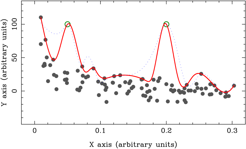
Figure 15: Example of constrained boundary fit, using adaptive splines with the same data employed in Figs. 2, 4 and 6. The boundary (red line) has been forced to pass through the points marked with open circles (green), namely (0.05,100) and (0.20,100). To give an important weight to the two constraints in Eq. (13), the value of the penalisation factor has been set to $\Lambda=10^{6}$. The dotted blue line is the same fit, but introducing two new additional constraints, in particular forcing the derivatives to be zero at the same fixed points.

As an example, Fig. 15 displays the upper boundary limit computed using adaptive splines for the same data previously employed in Figs. 2, 4 and 6, but arbitrarily forcing the fit to pass through the two fixed points (0.05,100) and (0.20,100), marked in the figure with the green open circles. The constrained fit (thick continuos red line) has been determined by introducing the two equality constraints

$$\begin{array}[]{@{}ll}c_{1}:&y(x=0.05)-100=0,\quad\mbox{and}\\ c_{2}:&y(x=0.20)-100=0.\end{array}$$ (14)

The displayed fit was computed using a penalisation factor $\Lambda=10^{6}$, with an asymmetry coefficient $\xi=1000$, $N_{\mbox{\scriptsize knots}}=15$, $N_{\mbox{\scriptsize maxiter}}=1000$ iterations, $N_{\mbox{\scriptsize refine}}=20$ processes, $\alpha=2$, and $\beta=0$. For comparison, another fit (dotted blue line) has also been computed by introducing two more constraints, namely forcing the derivatives to be zero at the same points, i.e., $y^{\prime}(x=0.05)=0$ and $y^{\prime}(x=0.20)=0$. The resulting fit is clearly different, highlighting the importance of the introduction of the constraints.

Appendix B Normalisation of data ranges to reduce numerical errors

The appearance of numerical errors is one of the most important sources of problems when fitting functions, in particular polynomials, to any data set making use of a piece of software. The problems can be specially serious when handling large data sets, using high polynomial degrees, and employing different and large data ranges. Since the size of the data set is usually something that one does not want to modify, and the polynomial degree is also fixed by the nature of the data being modelled (furthermore in the case of cubic splines, where the polynomial degree is fixed), the easier way to reduce the impact of numerical errors is to normalise the data ranges prior to the fitting procedure. However, although this normalisation is a straightforward operation, the fitted coefficients cannot be directly employed to evaluate the sought function in the original data ranges. Previously it is necessary to properly transform those coefficients. This appendix provides the corresponding coefficient transformations for the case of the fitting to simple one-dimensional polynomials and to cubic splines.

B.1 Simple polynomials

Simple polynomials are typically expressed as

$$y=a_{0}+a_{1}x+a_{2}x^{2}+\cdots+a_{p}x^{p}.$$ (15)

Let’s consider that the ranges exhibited by the data in the corresponding coordinate axes are given by the intervals $[x_{\mbox{\scriptsize min}},x_{\mbox{\scriptsize max}}]$ and $[y_{\mbox{\scriptsize min}},y_{\mbox{\scriptsize max}}]$, and assume that one wants to normalise the data within these intervals into new ones given by $[\tilde{x}_{\mbox{\scriptsize min}},\tilde{x}_{\mbox{\scriptsize max}}]$ and $[\tilde{y}_{\mbox{\scriptsize min}},\tilde{y}_{\mbox{\scriptsize max}}]$, through a point-to-point mapping from the original intervals into the new ones,

$$\left[x_{\mbox{\scriptsize min}},x_{\mbox{\scriptsize max}}\right] \longrightarrow \left[\tilde{x}_{\mbox{\scriptsize min}},\tilde{x}_{\mbox{\scriptsize max}}\right],\quad\mbox{and}$$

$$\left[y_{\mbox{\scriptsize min}},y_{\mbox{\scriptsize max}}\right] \longrightarrow \left[\tilde{y}_{\mbox{\scriptsize min}},\tilde{y}_{\mbox{\scriptsize max}}\right]$$

For this purpose, linear transformations of the form

$$\tilde{x}=b_{x}x-c_{x}\quad\mbox{and}\quad\tilde{y}=b_{y}y-c_{y}$$ (16)

are appropriate, where $b$ and $c$ are constants ($b_{x}$ and $b_{y}$ are scaling factors, and $c_{x}$ and $c_{y}$ represent origin offsets in the normalised data ranges). The inverse transformations will be given by

$$x=\frac{\tilde{x}+c_{x}}{b_{x}}\quad\mbox{and}\quad y=\frac{\tilde{y}+c_{y}}{b_{y}}.$$ (17)

Assuming that the original and final intervals are not null (i.e., $x_{\mbox{\scriptsize min}}\neq x_{\mbox{\scriptsize max}}$, $\tilde{x}_{\mbox{\scriptsize min}}\neq\tilde{x}_{\mbox{\scriptsize max}}$, $y_{\mbox{\scriptsize min}}\neq y_{\mbox{\scriptsize max}}$ and $\tilde{y}_{\mbox{\scriptsize min}}\neq\tilde{y}_{\mbox{\scriptsize max}}$), it is trivial to show that the transformation constants are given by

$$b_{x} = \displaystyle\frac{\tilde{x}_{\mbox{\scriptsize max}}-\tilde{x}_{\mbox{\scriptsize min}}}{x_{\mbox{\scriptsize max}}-x_{\mbox{\scriptsize min}}},$$ (18)

$$c_{x} = \displaystyle\frac{\tilde{x}_{\mbox{\scriptsize max}}x_{\mbox{\scriptsize min}}-\tilde{x}_{\mbox{\scriptsize min}}x_{\mbox{\scriptsize max}}}{x_{\mbox{\scriptsize max}}-x_{\mbox{\scriptsize min}}},$$ (19)

and the analogue expressions for the coefficients of the $y$-axis transformation. For example, to perform all the arithmetical manipulations with small numbers, it is useful to choose $\tilde{x}_{\mbox{\scriptsize min}}=\tilde{y}_{\mbox{\scriptsize min}}\equiv-1$ and $\tilde{x}_{\mbox{\scriptsize max}}=\tilde{y}_{\mbox{\scriptsize max}}\equiv+1$, which leads to

$$b_{x} = \displaystyle\frac{2}{x_{\mbox{\scriptsize max}}-x_{\mbox{\scriptsize min}}},$$ (20)

$$c_{x} = \displaystyle\frac{x_{\mbox{\scriptsize min}}+x_{\mbox{\scriptsize max}}}{x_{\mbox{\scriptsize max}}-x_{\mbox{\scriptsize min}}},$$ (21)

and the analogue expressions for $b_{y}$ and $c_{y}$.

Once the data have been properly normalised in both axes following the transformations given in Eq. (16), it is possible to carry out the fitting procedure, which provides the resulting polynomial expressed in terms of the transformed data ranges as

$$\tilde{y}=\tilde{a}_{0}+\tilde{a}_{1}\tilde{x}+\tilde{a}_{2}\tilde{x}^{2}+\cdots+\tilde{a}_{p}\tilde{x}^{p}.$$ (22)

At this point, the relevant question is how to transform the fitted coefficients $\tilde{a}_{0},\tilde{a_{1}},\ldots,\tilde{a}_{p}$ into the coefficients $a_{0},a_{1},\ldots,a_{p}$ corresponding to the same polynomial defined over the original data ranges. By substituting the relations given in Eq. (16) in the previous expression one directly obtains

$$\begin{array}[]{@{}l@{\;}c@{\;}l}(b_{y}y-c_{y})&=&\tilde{a}_{0}+\tilde{a}_{1}(b_{x}x-c_{x})+\tilde{a}_{2}(b_{x}x-c_{x})^{2}+\\ &&+\cdots+\tilde{a}_{p}(b_{x}x-c_{x})^{p}.\end{array}$$ (23)

Remembering that

$$(b_{x}x-c_{x})^{m}=\displaystyle\sum_{n=0}^{m}\left(\begin{array}[]{@{}c@{}}m\\ n\end{array}\right)(b_{x}x)^{m-n}(-c_{x})^{n},$$ (24)

with the binomial coefficient computed as

$$\left(\begin{array}[]{@{}c@{}}m\\ n\end{array}\right)=\frac{m!}{n!\;(m-n)!},$$ (25)

and comparing the substitution of Eq. (24) and Eq. (25) into Eq. (23) with the expression given in Eq. (15), it is not difficult to show that if one defines

$$h_{i}\equiv\displaystyle\sum_{j=i}^{p}\tilde{a}_{j}\left(\begin{array}[]{@{}c@{}}j\\ j-i\end{array}\right)(b_{x})^{i}(-c_{x})^{j-i}$$ (26)

the sought coefficients will be given by

$$a_{i}=\left\{\begin{array}[]{cl}\displaystyle\frac{h_{0}+c_{y}}{b_{y}}&\mbox{for}\;i=0\\ &\\ \displaystyle\frac{h_{i}}{b_{y}}&\mbox{with}\;i=1,\ldots,p\end{array}\right.$$ (27)

In the particular case in which $c_{x}=0$, the above expressions simplify to

$$a_{i}=\left\{\begin{array}[]{cl}\displaystyle\frac{\tilde{a}_{0}+c_{y}}{b_{y}}&\mbox{for}\;i=0\\ &\\ \displaystyle\frac{\tilde{a}_{i}b_{x}^{i}}{b_{y}}&\mbox{with}\;i=1,\ldots,p\end{array}\right.$$ (28)

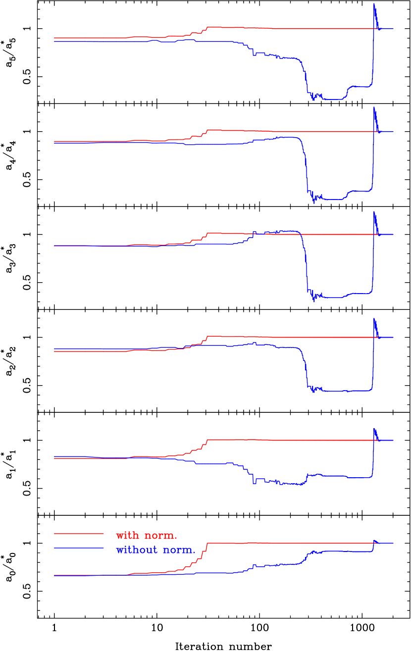
Figure 16: Variation in the fitted coefficients, as a function of the number of iterations, for the upper boundary fit (5th order polynomial) shown in Fig. 2a. This plot is the same than Fig. 3, but in this case analysing the impact of the normalisation of the data ranges prior to the boundary determination. Each panel represents the coefficient value at a given iteration ($a_{i}$, with $i=0,\ldots,5$, from bottom to top) divided by $a_{i}^{*}$, the final value derived after $N_{\mbox{\scriptsize maxiter}}=2000$ iterations. The same $y$-axis range is employed in all the plots. The red line shows the results when applying the normalisation, and the blue line indicates the coefficient variations when this normalisation is not applied. In both cases $\xi=1000$, $\alpha=2$ and $\beta=0$ were used. Note that the plot $x$-scale is in logarithmic units.

The normalisation of the data ranges has several advantages. Fig. 16 (similar to Fig. 3) shows the impact of data normalisation on the convergence properties of the fitted coefficients, as a function of the number of iterations, for the upper boundary fit (5th order polynomial) shown in Fig. 2a. The red line, corresponding to the results when the normalisation is applied prior to the boundary fitting, indicates that after $N_{\mbox{\scriptsize maxiter}}\sim 140$, the coefficients have converged. The situation is much worse when the normalisation is not applied, as illustrated by the blue line. In this case the convergence is only reached after $N_{\mbox{\scriptsize maxiter}}\sim 1450$ iterations, ten times more than when using the normalisation. In addition, the ranges spanned by the coefficient values along the minimisation procedure are narrower when the data ranges have been previously normalised.

Figure 17: Example of the appearance of numerical errors in the boundary fitting with simple polynomials. The fitted data set consists in 10000 points randomly drawn from the function $y=\sin(1.5x)/(1+x)$ for $x\in[0,2\pi]$, assuming a Gaussian error $\sigma=0.02$ in the $y$-axis, and where prior to the data fitting the $(x,y)$ coordinates were transformed using $x_{\mbox{\scriptsize fit}}=1000+500\;x_{\mbox{\scriptsize original}}$ and $y_{\mbox{\scriptsize fit}}=1000\;y_{\mbox{\scriptsize original}}$ in order to artificially enlarge the data ranges. Panel (a): bootstrapped data and fitted boundaries. Panel (b): residuals relative to the original sinusoidal function. In both panels the lines indicate the resulting fits for different polynomial degrees and normalisation strategies (in all the cases $\xi=1000$, $\alpha=2$ and $\beta=0$ were employed). The continuous red lines are the boundaries obtained using polynomials of degree 10 and normalising the data ranges prior to the fitting procedure. The green and blue lines correspond to the fits obtained by fitting polynomials of degrees 9 and 8, respectively, without normalising the data ranges. Using the original data ranges the boundary fits start to depart from the expected location due to numerical errors for polynomials of degree 9. However polynomials of degree 10 are still an option when the data ranges are previously normalised.

Fig. 17 exemplifies the appearance of numerical errors that takes place when increasing the polynomial degree during the fitting of a reasonably large data set. In this case 10000 points are fitted employing upper and lower boundaries with simple polynomials of degree 10 (red lines) after normalising the data ranges using the coefficients given in Eqs. (20) and (21) (with the analogue expressions for the $y$-axis coefficients) prior to the numerical minimisation. When the data ranges are not normalised, the fitting to polynomials of degree 10 gives non-sense results. Only polynomials of degree less or equal than 9 are computable. And for the case of degree 9 the results are unsatisfactory (green lines), being the polynomials of degree 8 (blue lines) the first reasonable boundaries while fitting the data preserving their original ranges. Thus in this particular example the normalisation of the data ranges allows to extend the fitted polynomial degree in two units.

B.2 Cubic splines

Normalisation of the data ranges is also important for the computation of cubic splines, in particular for the boundary fitting to adaptive splines described in Section 3. In that section the functional form of a fit to set of $N_{\mbox{\scriptsize knots}}$ was expressed as

$$\begin{array}[]{@{}r@{\;}l}y=&s_{3}(k)[x-x_{\mbox{\scriptsize knot}}(k)]^{3}+s_{2}(k)[x-x_{\mbox{\scriptsize knot}}(k)]^{2}+\\ +&s_{1}(k)[x-x_{\mbox{\scriptsize knot}}(k)]+s_{0}(k),\end{array}$$

where ($x_{\mbox{\scriptsize knot}}(k),y_{\mbox{\scriptsize knot}}(k)$) are the $(x,y)$ coordinates of the $k^{\mbox{\scriptsize th}}$ knot, and $s_{0}(k)$, $s_{1}(k)$, $s_{2}(k)$, and $s_{3}(k)$ are the corresponding spline coefficients for $x\in[x_{\mbox{\scriptsize knot}}(k),x_{\mbox{\scriptsize knot}}(k+1)]$, with $k=1,\ldots,N_{\mbox{\scriptsize knots}}-1$.

Using the same nomenclature previously employed for the case of simple polynomials, the result of a fit to cubic splines performed over normalised data ranges should be written as

$$\begin{array}[]{@{}r@{\;}l}\tilde{y}=&\tilde{s}_{3}(k)[\tilde{x}-\tilde{x}_{\mbox{\scriptsize knot}}(k)]^{3}+\tilde{s}_{2}(k)[\tilde{x}-\tilde{x}_{\mbox{\scriptsize knot}}(k)]^{2}+\\ +&\tilde{s}_{1}(k)[\tilde{x}-\tilde{x}_{\mbox{\scriptsize knot}}(k)]+\tilde{s}_{0}(k).\end{array}$$

Following a similar reasoning to that used previously, it is straightforward to see that the sought transformations are

$$s_{i}(k)=\left\{\begin{array}[]{cl}\displaystyle\frac{\tilde{s}_{0}(k)+c_{y}}{b_{y}}&\mbox{for}\;i=0\\ &\\ \displaystyle\frac{\tilde{s}_{i}(k)b_{x}^{i}}{b_{y}}&\mbox{with}\;i=1,\ldots,3\end{array}\right.$$ (29)

where $k=1,\ldots,N_{\mbox{\scriptsize knots}}-1$. Note that these transformations are identical to Eq. (28). This is not surprising considering that splines are polynomials and that the adopted functional form given in Eq. (B.2) is actually providing the $y(x)$ coordinate as a function of the distance between the considered $x$ and corresponding value $x_{\mbox{\scriptsize knot}}(k)$ for the nearest knot placed at the left side of $x$. Thus, the $c_{x}$ coefficient is not relevant here.

B.3 A word of caution

Although the method described in this appendix can help in some circumstances to perform fits with larger data sets or higher polynomial degrees than without any normalisation of the data ranges, it is important to keep in mind that such normalisation does not always produce the expected results and that numerical errors appear in any case sooner or later if one tries to use excessively large data sets or very high values for the polynomial degrees.

Anyhow, the fact that the normalisation of the data ranges can facilitate the boundary determination of large data sets or to use higher polynomial degrees justifies the effort of checking whether such normalisation is of any help. Sometimes, to extend the polynomial degrees by even just a few units can be enough to solve the particular problem one is dealing with. The program BoundFit incorporates the normalisation of the data prior to the boundary fitting as an option.

References

- Bazaraa, Sherali & Shetty (1993) Bazaraa M.S., Sherali H.D., Shetty C.M., 1993, Nonlinear programming: theory and algorithms, John Wiley & Sons, 2nd edition
- Cardiel (1999) Cardiel N., 1999, PhD Thesis, Universidad Complutense de Madrid
- Cardiel et al. (2003) Cardiel N., Elbaz D., Schiavon R.P., Willmer C.N.A., Koo D.C,. Phillips A.C., Gallego J., 2003, ApJ, 584, 76
- Faber (1973) Faber S.M., 1973, ApJ, 179, 731
- Faber et al. (1977) Faber S.M., Burstein D., Dressler A., 1977, AJ, 82, 941 179, 731
- Fletcher (2007) Fletcher R., 2007, Practical methods of optimization, John Wiley & Sons, 2nd edition
- Geisler (1984) Geisler D., 1984, PASP, 96, 723
- Gerald & Wheatley (1989) Gerald C.F., Wheatley P.O., 1989, Applied Numerical Analysis, Addison-Wesley, 4th edition
- Gill, Murray & Wright (1989) Gill P.E., Murray W., Wright M.H., 1989, Practical optimization, Academic Press
- Haupt & Haupt (2004) Haupt R.L., Haupt S.E., 2004, Practical Genetic Algorithms, Wiley-Interscience, 2nd edition
- Nelder & Mead (1965) Nelder J.A., Mead R., 1965, Computer Journal, 7, 308
- Nocedal & Wright (2006) Nocedal J., Wright S.J., 2006, Numerical Optimization, Springer Verlag, 2nd edition
- Press et al. (2002) Press W.H., Teukolsky S.A., Vetterling W.T., Flannery B.P., 2002, Numerical Recipes in C++, Cambridge University Press, 2nd edition
- Rao (1978) Rao S.S., 1978, Optimization: theory and applications, Wiley Eastern Limited
- Rich (1988) Rich R.M., 1988, AJ, 95, 828
- Rogers et al. (2008) Rogers B., Ferreras I., Peletier R., Silk J., 2008, MNRAS, in press (astro-ph/0812.2029)
- Sánchez-Blázquez et al. (2006) Sánchez-Bázquez P., Peletier R.F., Jiménez-Vicente J., Cardiel N., Cenarro A.J., Falcón-Barroso J., Gorgas J., Selam S., Vazdekis A., MNRAS, 371, 703
- Rose (1994) Rose J.A., 1994, AJ, 107, 206
- Trager (1997) Trager S.C., 1997, Ph.D. Thesis, University of California, Santa Cruz
- Vazdekis & Arimoto (1999) Vazdekis A., Arimoto N., 1999, ApJ, 525, 144
- Whitford & Rich (1983) Whitford A.E., Rich R.M., 1983, ApJ, 274, 723
- Worthey & Ottaviani (1997) Whorthey G., Ottaviani D.L., 1997, ApJS, 111, 377