Scaling of the fidelity susceptibility in a disordered quantum spin chain

Abstract

The phase diagram of a quantum XY spin chain with Gaussian-distributed random anisotropies and transverse fields is investigated, with focus on the fidelity susceptibility, a recently introduced quantum information theoretical measure. Monitoring the finite-size scaling of the probability distribution of this quantity as well as its average and typical values, we detect a disorder-induced disappearance of criticality and the emergence of Griffiths phases in this model. It is found that the fidelity susceptibility is not self-averaging near the disorder-free quantum critical lines. At the Ising critical point the fidelity susceptibility scales as a disorder-strength independent stretched exponential of the system size, in contrast with the quadratic scaling at the corresponding point in the disorder-free XY chain. Along the line where the average anisotropy vanishes the fidelity susceptibility appears to scale extensively, whereas in the disorder-free case this point is quantum critical with quadratic finite-size scaling.

I Introduction

In the last few years, tools from the field of quantum information theory have found extensive use in the study of the phase diagrams of quantum systems. One such technique, the fidelity approach to Quantum Phase Transitions (QPTs) has been successfully applied to various systems possessing quantum critical points PZ ; ZhBa ; ZhZhLi ; Zh (see Gu for a review). This technique can be generalized to finite-temperature systems ZQWS ; ZCVG , classical phase transitions QC , and topological phase transitions HaZhHa ; AbZa ; AbHaZa ; YaGuSu ; GaAbHa ; Eriksson .

In a recent letter GJHZ we have studied the fidelity in the context of disordered quantum systems. The physics peculiar to disordered quantum systems is reflected in the properties of the fidelity, a quantity not previously used to investigate such systems. Here we study the scaling behavior and provide details concerning the zero-temperature phase diagram of the disordered quantum XY model in a transverse field, a prototypical model in the context of disordered quantum systems.

The paper is organized as follows. Section II is devoted to defining the model, along with a review of known results about its phase diagram and the basics of the fidelity approach. Section III presents the numerical results of our study and discusses the main features of the fidelity for disordered quantum chains. Our conclusions are presented in Section IV.

II Method and model

It is known that disorder can have interesting effects on a system’s phase diagram IgMo . In particular, Griffiths phases may arise as a result of the randomness Gri . Here we study the disordered anisotropic quantum XY spin chain in a random transverse field, a model where the disorder-free case can be analytically solved LiScMa and for which some exact results are known in the disordered case McK ; BMcK . Its Hamiltonian is given by

$$H=-\sum_{i=1}^{L}\frac{1+\gamma_{i}}{2}\sigma_{i}^{x}\sigma_{i+1}^{x}+\frac{1-\gamma_{i}}{2}\sigma_{i}^{y}\sigma_{i+1}^{y}+\lambda_{i}\sigma_{i}^{z},$$ (1)

where $\sigma_{i}^{\left\{x,y,z\right\}}$ are Pauli matrices, and the fields $\lambda_{i}$ and anisotropies $\gamma_{i}$ are independent Gaussian-distributed random variables. The average field and anisotropy are denoted by $\lambda$ and $\gamma$, respectively. The variance is taken to be the same for both the field and anisotropy distributions.

The Jordan-Wigner transformation maps this system onto quasi-free spinless fermions LiScMa . Neglecting the boundary term and taking the system to be closed in the fermion index, we obtain a Hamiltonian of the form

$$H=\sum_{i,j=1}^{L}c^{\dagger}_{i}A_{ij}c_{j}+\frac{1}{2}\sum_{i,j=1}^{L}\left(c^{\dagger}_{i}B_{ij}c^{\dagger}_{j}+c_{j}B_{ij}c_{i}\right),$$ (2)

where $A$ and $B$ are symmetric and antisymmetric real $L\times L$ matrices, respectively. Explicitly: $A_{ij}=-(2\lambda_{i}\delta_{ij}+\delta_{i,j+1}+\delta_{i+1,j})$, $A_{1L}=A_{L1}=-1$ and $B_{ij}=\gamma_{j}\delta_{i,j+1}-\gamma_{i}\delta_{i+1,j}$, $B_{1L}=\gamma_{L}=-B_{L1}$.

The Hamiltonian may be rewritten in terms of the matrix $Z\equiv A-B$, which contains all information about the system. Performing the polar decomposition of $Z$ we obtain the matrices $\Lambda$ and $T$ such that $Z=\Lambda T$, where $\Lambda$ is a positive semi-definite matrix and $T$ is unitary. From the eigenvalues of $\Lambda$ one obtains the single-particle energy spectrum CGZ .

For systems at zero temperature, the fidelity is simply the absolute value of the overlap between ground states corresponding to nearby points in parameter space. Near a quantum critical point the ground state changes rapidly for small shifts in the tuning parameters, an effect which is reflected in a corresponding decrease of the fidelity.

The ground state fidelity can be cast in terms of the unitary matrix $T$ in the following way ZCG

$$F(Z,\tilde{Z})=\sqrt{|\det{\frac{T+\tilde{T}}{2}}|},$$ (3)

where $T$ and $\tilde{T}$ are respectively the unitary parts of the matrices $Z\equiv Z(x)$ and $\tilde{Z}\equiv Z(x^{\prime})$, evaluated at the model parameters $x$ and $x^{\prime}$. The corresponding fidelity susceptibility is defined as YouLiGu ; CVZ

$$\chi(x)=\lim_{\Delta x\rightarrow 0}\frac{-2\ln{F(x,x+\Delta x)}}{\Delta x^{2}},$$ (4)

and can be written in terms of the unitary matrix $T$ as

$$\chi(x)=\frac{1}{8}\|\partial_{x}T\|_{F}^{2},$$ (5)

where $\|\cdot\|_{F}$ is the Frobenius norm. For a derivation of Eq. (5) see the Appendix.

We evaluate the fidelity susceptibility using (5) by performing a singular value decomposition of $Z$

$$Z=U\Sigma V^{\dagger}=(U\Sigma U^{\dagger})(UV^{\dagger})=\Lambda T,$$

where $U$ and $V$ are unitary matrices. Note that the fidelity susceptibility is defined for infinitesimally separated points along any chosen direction in parameter space.

II.1 Disorder-free case

Before considering the effects of disorder in the XY chain, let us first recall the behavior of the fidelity susceptibility for the disorder-free case, where $\lambda_{i}=\lambda,\gamma_{i}=\gamma,\forall i\in\{1,...,L\}$ PZ . The system can then be found in one of three phases. For $|\lambda|>1$ it is paramagnetic, and for $|\lambda|<1$ and $\gamma>0$ ($\gamma<0$) the system is ferromagnetic along the $x$- direction ($y$-direction). The boundary between any two of these phases is a quantum-critical line corresponding to a second-order quantum phase transition. Here, we refer to the transition driven by the magnetic field as the Ising transition, and to the transition driven by the anisotropy coupling as the anisotropy transition. At the quantum-critical points there is an avoided level crossing between the ground state and the first excited state. As shown in Figs. 1(a) and 1(b), one observes a maximum of the fidelity susceptibility at both the Ising and anisotropy critical lines.

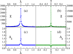
Figure 1: (color online) The disorder-free case: (a) Fidelity susceptibility near the Ising transition, with $\gamma=1$ and system size $L=500$. (b) Near the anisotropy transition, with $\lambda=0.5$ and system size $L=500$. (c) Finite-size scaling dimension of the fidelity susceptibility near the Ising transition, with $\gamma=1$. The sizes considered range from $L=100$ to $700$, with $\chi\sim L^{\Delta_{\chi}}$. (d) Finite-size scaling of the fidelity susceptibility near the anisotropy transition, with $\lambda=0.5$. The sizes considered range from $L=100$ to $600$.

Moreover, the finite-size scaling dimension of the fidelity susceptiblity in Figs. 1(c) and 1(d) show it to be extensive away from criticality and superextensive (scaling quadratically with $L$) at the critical points. This scaling behavior holds for both the Ising and anisotropy critical lines. The apparent subextensive scaling in the immediate vicinity of the anisotropy critical point is a numerical artifact due to the narrowing of the fidelity susceptibility peak as the system size grows. The Ising transition does not show this behavior, since the narrowing appears to occur more slowly than for the anisotropy transition.

It has been shown CVZ , for translationally invariant systems, that superextensive finite-size scaling of the fidelity susceptibility implies a vanishing gap and therefore quantum criticality. As a result, for clean systems the points in parameter space corresponding to superextensive scaling of this quantity mark quantum critical regions. When randomness is introduced, translational invariance is lost, and hence superextensive scaling of the fidelity susceptibility does not necessarily imply quantum criticality. As discussed before, we find that locations of superextensive scaling reveal more general behavior beyond quantum criticality, namely Griffiths phenomena Gri .

II.2 Random XY chain

The effects of disorder on the physics of quantum magnets has been studied mainly using the strong-disorder renormalization group technique (SDRG) DasMa ; Fis1 ; Fis2 . A different approach has been used in the work of McKenzie and Bunder McK ; BMcK , where the critical behavior of the disordered XY chain has been studied using a mapping to random-mass Dirac equations. The properties of the solutions of these equations imply the disappearance of the anisotropy transition in the presence of disorder. Furthermore, Griffiths phases are predicted to appear both around the Ising critical line and the anisotropy $\gamma=0$ line. These results, together with the analysis performed by Fisher Fis1 ; Fis2 , are significant since they analytically show the drastic effects that disorder can have on the critical properties of a quantum system.

At fixed $\gamma$ the XY random chain is closely related to the random transverse-field Ising chain (RTFIC), which is another prototypical model for disordered quantum systems Fis2 . Since the RTFIC is representative of the universality class of Ising transitions for all values of $\gamma$, let us review what is known for this model. The Hamiltonian of the RTFIC is $H=-\sum_{i=0}^{L-1}\left[J_{i}\sigma_{i}^{x}\sigma_{i+1}^{x}+h_{i}\sigma_{i}^{z}\right],$ where $J_{i}$ and $h_{i}$ are random couplings and fields respectively. The system is critical when the average value of the field equals the average value of the coupling. Using the SDRG one obtains that, at the quantum critical point, the time scale $\tau$ and the length scale $L$ are related by $\ln{\tau}\sim L^{1/2}$. This results in an infinite value for the dynamical exponent $z$ at criticality Fis2 . The distribution of the logarithm of the energy gap $\epsilon$ at criticality broadens with increasing system size, in accordance with the scaling relation $\ln{\epsilon}\sim-L^{1/2}$ YoRi . In the vicinity of the critical point the distribution of relaxation times is broad due to the presence of a Griffiths phase, characterized by a non-universal dynamical exponent $z$ depending on the distance from the critical point. This dependence can be used as an indicator for the Griffiths phase.

In GJHZ a study of the phase diagram of a random XY spin chain in a random transverse field was performed using the fidelity approach. There it was shown that superextensive finite-size scaling of $\chi$ signals the presence of a quantum phase transition close to the Ising critical line, while the minimum in $\chi$ close to the anisotropy $\gamma=0$ line is consistent with the absence of a phase transition in that parameter region, see Figs. 2(a) and (b).

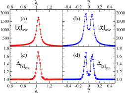
Figure 2: (color online) (a) Average fidelity susceptibility near the Ising transition, for $L=500$, $\gamma=1$, and $\sigma=0.3$, (b) Average $\chi$ near the $\gamma=0$ line, for $L=500$, $\lambda=0.5$, and $\sigma=0.3$, (c) Scaling dimension of $\chi$ for the same set of parameters near the Ising line, considering $L\in\{100,200,300,400,500\}$, (d) Scaling dimension of $\chi$ for the same set of parameters near the $\gamma=0$ line, considering $L\in\{100,200,300,400,500\}$.

The Griffiths phases of the model manifest themselves in a non-universal dependence of the finite-size scaling dimension $\Delta_{\chi}$ of the fidelity susceptibility on the distance from the disorder-free critical point, see Figs. 2(c) and (d). The relation between the dynamical scaling exponent $z$ and the scaling dimension of $\chi$ CVZ

$$\Delta_{\chi}=2z+2-2\Delta_{O}$$ (6)

establishes the connection between the fidelity susceptibility and the Griffiths phase. In Eq.(6) $\Delta_{O}$ is the scaling dimension of the relevant operator driving the transition. Eq. (6) implies a non-universal scaling dimension for the fidelity susceptibility $\Delta_{\chi}$, provided that the behavior of the unknown scaling dimension $\Delta_{O}$ does not exactly cancel that of the dynamical exponent. In the following we would like to study, using other methods, the extent of the Griffiths phase for this model. In particular, we would like to verify that the entrance into a Griffiths phase is indeed reflected by a changing scaling behavior of the fidelity susceptibility.

In our numerical analysis we consider system sizes $L\in\{100,200,300,400,500\}$ and for each system size we compute $10^{4}$ disorder realizations. We take the external fields (anisotropies) to be independent and identically distributed Gaussian random variables with standard deviation $\sigma$ and mean $\lambda$ ($\gamma$). We consider the range of values $\{0.1,0.2,0.3,0.4\}$ for the standard deviation $\sigma$. This disorder strength can be considered strong with respect to the value of the other parameters. We denote with $\left[\cdot\right]_{\textrm{ave}}$ the arithmetic mean over all $10^{4}$ disorder realizations.

The width of the Griffiths phase for the XY model with weak Gaussian disorder in the continuum limit is known due to the work of McKenzie McK . Let us denote the distance from criticality with $\delta$, where $\delta=0$ corresponds to the points in parameter space where the pure system is critical. From McK one can compute that near the Ising transition, where the field $\lambda$ drives the transition, $\delta=\frac{|\gamma|(\lambda-1)}{\sigma^{2}}$, while near the anisotropy line $\delta=\frac{\gamma(1-\lambda^{2})}{\sigma^{2}}$.

For the so-called commensurate case, which corresponds to the Ising transition for this system since we have disorder in both the field and anisotropy, McKenzie showed that the disorder-averaged density of states $\left[\rho(E)\right]_{\rm{ave}}/\rho_{0}$ diverges at zero energy within the range $|\delta|<1/2$ away from the critical point McK . Here $\rho_{0}$ is the “high-energy” density of states. This divergence implies that the gap distribution function $P(\Delta E)$ also diverges at zero energy, since a large density of states means a vanishingly small gap. Note that a diverging probability of having a vanishing gap does not necessarily imply that the density of states is also divergent, since the gap distribution only provides information about the position of the first excited energy level relative to the ground state energy. However, since a diverging gap distribution should be expected to occur as a result of a divergence of the low-energy density of states, we will use it to give a rough estimate of the extent of the Griffiths phase.

For the incommensurate case, which includes the anisotropy transition, $\left[\rho(E=0)\right]_{\rm{ave}}/\rho_{0}$ is of the order of unity for some range of parameters about $\delta=0$, implying effective gaplessness, and $\left[\rho(E=0)\right]_{\rm{ave}}/\rho_{0}$ is much smaller than unity for $|\delta|>>1$, giving an effectively finite gap McK . Note that the boundary of the Griffiths phase in this region is expected to be less defined than near the Ising transition, since the zero-energy density of states does not diverge at any value of $\delta$.

These results apply for the case of weak disorder, but we consider a range of moderate to strong disorder strengths. In order to compare with the results of McKenzie for the Griffiths phase extent, we propose a rough criterion for determining the extent of the Griffiths phase using the gap distribution. Assume that the Griffiths phase lies within the range of parameter values for which the distribution $P(\Delta E)$ has a maximum for $\Delta E=0$. At some point away from criticality the distribution maximum moves away from zero, eventually becoming approximately Gaussian far from the disorder-free critical point. We have determined the range of parameters for which $P(\Delta E)$ has a maximum at zero gap. The width of this range of parameters is independent of system size and scales with the variance of the coupling or field distributions, in accordance with the result of McK . However, this criterion gives an extent several times larger than the McKenzie value, around both the Ising and $\gamma=0$ lines. This difference may be due to strong disorder or, rather, the result of an overestimation of the Griffiths phase extent since the distribution $P(\Delta E)$ having a maximum at zero does not directly imply a divergent zero-energy density of states. Nonetheless, consistency between different estimations of the Griffiths phase extent support the validity, at least qualitatively, of this approach.

Fig.(3) shows the gap distribution in the vicinity of the $\gamma=0$ line. For small anisotropies the distribution has a pronounced peak at zero gap. Moving away from the anisotropy line, the distribution develops a peak slightly away from $\Delta E=0$, and for larger anisotropies the distribution becomes Gaussian with a vanishing probability of having zero gap. Similar behavior holds for the Ising transition as the average field $\lambda$ is adjusted away from the finite-size pseudocritical point.

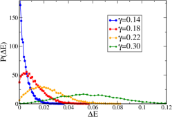
Figure 3: (color online) Gap distribution near the anisotropy line, with $\lambda=0.5$, $\sigma=0.3$, and system size $L=500$. Plotted distributions are for $\gamma=0.14,0.18,0.22,$ and $0.30$.

III Results

III.1 Average and typical values

In computing the average of some physical quantity, namely the arithmetic mean over many disorder realizations, any rare but large values will significantly affect the result. On the other hand, the geometric mean over disorder realizations gives a more representative measure of the typical values of the physical quantity. Recall that the arithmetic mean provides an upper bound for the geometric mean when averaging over a set of positive values, and the two are equal only when taking the mean of a constant set of values.

To observe the presence of large fluctuations in the fidelity susceptibility, we plot in Fig. 4(a) the disorder-averaged as well as typical fidelity susceptibility in the vicinity of the Ising critical point for a disorder strength $\sigma=0.3$. Notice that in the vicinity of the critical point the average becomes significantly larger than the typical value, indicating that there are instances of large fidelity susceptibilities that skew the arithmetic average towards a greater value.

Near the anisotropy line, as shown in Fig. 4(b), there are also regions where the average fidelity susceptibility becomes much larger than the typical value, but now the positions of largest difference do not correspond to a critical point. Indeed, at the point $\gamma=0$, which in the disorder-free case is critical, the average-typical difference is much smaller than it is at the two offset peaks. This is evidence for the disappearance of the anisotropy transition as a result of the disorder.

For translationally invariant systems, which are disorder-free, it has been shown that superextensive finite-size scaling of the fidelity susceptibility implies quantum criticality CVZ . The disordered XY chain does not have translational invariance, so locations of superextensive scaling do not necessarily imply criticality. However, it is still useful to consider finite-size scaling, since comparison with the disorder-free case may suggest in what way the phase diagram changes as a result of disorder. Fig.(5) shows the finite-size scaling dimension of the typical fidelity susceptibility near the Ising transition. The locations of the maxima of the typical fidelity susceptibility and finite-size scaling dimension coincide, and are shifted from the pure pseudocritical point due to finite-size effects. Also, the maximum scaling dimension obtained with disorder is smaller than the pure case of quadratic scaling in $L$, and this maximum value decreases with increased disorder strength.

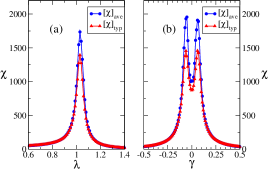
Figure 4: (color online) Average (blue) and typical (red) fidelity susceptibility about: (a) the Ising line, for $\gamma=1$, $L=500$, and $\sigma=0.3$ (b) the $\gamma=0$ line, for $\lambda=0.5$, $L=500$, and $\sigma=0.3$.

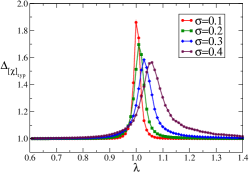
Figure 5: (color online) Finite-size scaling dimension of the typical fidelity susceptibility about the Ising transition, for $\gamma=1$, for $\sigma\in\{0.1,0.2,0.3,0.4\}$. Scaling fit considered system sizes $L=200,300,400,500$, with $\chi\sim L^{\Delta_{\left[\chi\right]_{typ}}}$ assumed.

In Fig.(6), the finite-size scaling dimension of $\chi$ around the anisotropy line $\gamma=0$ is shown for the same set of disorder strengths. Notice that the scaling depends on distance from the $\gamma=0$ line and at $\gamma=0$ the scaling is approximately extensive, as it is when far from the anisotropy line. For sufficiently small disorder and system size there may appear to be only a single peak in the typical fidelity susceptibility at $\gamma=0$, suggesting that for these finite systems emergent criticality is still felt even though the quantum phase transition in the thermodynamic limit disappears as a result of the disorder. However, increasing the system size reveals a double peak with a peak offset which grows with the strength of the disorder. In both the Ising and anisotropy regions, the width of the parameter interval giving scaling dimensions larger than a particular value scales approximately with the variance of the disorder distribution. This scaling behavior agrees with that given by the previously mentioned gap distribution criterion for the Griffiths phase.

In Fig.(7) the disorder-averaged gap is plotted for the four disorder strengths. The behavior of the gap corresponds closely with that of the fidelity susceptibility, in that the average gap minima have the same location as the typical $\chi$ maxima. Note that the vicinity of the Ising critical line and the $\gamma=0$ line are regions of effective gaplessness which we associate with quantum criticality or Griffiths phases.

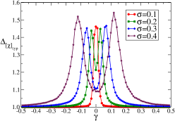
Figure 6: (color online) Finite-size scaling dimension of the typical fidelity susceptibility about the anisotropy line, for $\lambda=0.5$, for $\sigma\in\{0.1,0.2,0.3,0.4\}$. Scaling fit considered system sizes $L=100,200,300,400,500$, with $\chi\sim L^{\Delta_{\left[\chi\right]_{typ}}}$ assumed.

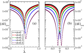
Figure 7: (color online) (a) Disorder-averaged gap near the Ising transition for disorder strengths $\sigma\in\{0,0.1,0.2,0.3,0.4\}$, $L=500$, and $\gamma=1$. (b) Disorder-averaged gap near the $\gamma=0$ line for the same range of disorder strengths, $L=500$, and $\lambda=0.5$.

An experiment on such a disordered system would consider only one particular realization of disorder, and as a result would not necessarily observe the disorder-averaged value of an observable but rather a typical value. Here, we would like to study whether a measurement of the fidelity susceptibility for a large system coincides with the average value, and to do this we must see for what conditions $\chi$ is a self-averaging quantity AH . Consider the quantity $R_{\chi}(x,L)=\textrm{Var}[\chi(x)]/[\chi(x)]_{\rm{ave}}^{2}$. We expect that $R_{\chi}(x,L)$ for fixed $x$ will scale as a power law in the system size $L$, $R_{\chi}\sim L^{b}$. If $b=-1$ then we say $\chi$ is self-averaging, if $b<0$ then $\chi$ is weakly self-averaging, and if $b>0$ then $\chi$ is not self-averaging. In Fig.(8) we indicate the regions for which $\chi$ is self-averaging, weakly self-averaging and non-self-averaging for various disorder strengths near the Ising transition as well as the $\gamma=0$ line.

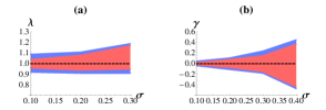
Figure 8: (color online) Regions about the Ising transition (a) and anisotropy line (b) for which $\chi$ is weakly self-averaging (blue) and non-self-averaging (orange), as a function of disorder strength $\sigma$. Outside these regions $\chi$ is self-averaging.

III.2 Fidelity susceptibility distributions

III.2.1 Near the Ising line

Far from the Ising critical line, the distribution of the fidelity susceptibility is Gaussian, see Fig.(9). However, in the vicinity of the Griffiths phase and the critical point the distribution is non-Gaussian, developing a slowly-decaying tail towards large fidelity susceptibilities, as shown in Fig.(10). This tail reflects the presence of rare but large fidelity susceptibilities, and is expected to arise either in a Griffiths phase or in a quantum critical region.

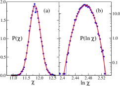
Figure 9: (color online) (a) Distribution of $\chi$ far from the Ising critical point, with $\lambda=1.49$ (blue). Overlaid is a Gaussian distribution function with the same mean and variance (red). (b) Distribution of $\ln\chi$ for the same parameters (blue) along with the corresponding distribution function of the logarithm of a Gaussian random variable. Here $\sigma=0.1$, $L=500$ and $\gamma=1$. This distribution is well described as Gaussian.

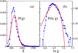
Figure 10: (color online) (a) Distribution near the Ising critical point, with $\lambda=1.03$ (blue). Overlaid is a Gaussian distribution function with the same mean and variance (red). (b) Distribution of $\ln\chi$ for the same parameters (blue) along with the corresponding distribution function of the logarithm of a Gaussian random variable. Here $\sigma=0.1$, $L=500$, and $\gamma=1$. Clearly this distribution is not Gaussian, as can be seen by the much slower dropoff of the tail towards large fidelity susceptibilities.

Now we explore how the distribution of the logarithm of the fidelity susceptibility changes as the system size is varied, with all other parameters fixed. Far from the Ising transition the distribution of $\ln(\chi)$ narrows with increasing system size, as shown in Fig. 11(a). The position of the peak of the distribution remains fixed for a rescaling $\chi\to\chi/L$ (see Fig. 11(b)), but the width of the distribution decreases slightly. Choosing a more general scaling assumption $\ln(\chi)\to L^{\beta}\ln(\chi/L^{\alpha})$ allows for an improved collapse of the distributions in this region, indicated in Fig. 11(c). The fit parameter $\alpha$ essentially translates the distribution, while the parameter $\beta$ adjusts the width. Such a scaling would imply a size dependence $\chi\sim L^{\alpha}\exp{L^{-\beta}}$, where $\alpha,\beta\geq 0$. However, for asymptotically large system sizes this would lead to subextensive scaling, and would thus not be expected to hold for all $L$. It appears that this apparent non-power-law scaling for the range of sizes we have considered may be due to finite-size effects, and we speculate that an assumption of extensive scaling would lead to an improved collapse for sufficiently large system sizes.

At the Ising pseudocritical point the distribution $P(\ln\chi)$ broadens significantly with increasing system size, and a rescaling $\ln(\chi)\to L^{-\beta}\ln(\chi)$ gives a good collapse for a value of the fit parameter $\beta=0.26$ (see Fig.(12)). This collapse and value of fit parameter holds for the pseudocritical points corresponding to all four disorder cases we have considered. A rescaling of this kind suggests that the fidelity susceptibility scales as a stretched exponential of the system size at the critical point rather than quadratically as in the pure XY chain. For the random transverse field Ising chain YoRi , it is known that the energy gap vanishes as $\Delta E\sim\exp{-\sqrt{L}}$ at the Ising critical point. Recalling the alternative expression for the fidelity susceptibility $\chi=\sum_{n\neq 0}{}\frac{|<n|\partial_{x}H|0>|^{2}}{|E_{n}-E_{0}|^{2}}$ YouLiGu , we expect that the first term in this series would dominate, and that the fidelity susceptibility might scale as $\chi\sim 1/(\Delta E)^{2}$. However, this crude argument appears not to be consistent with the scaling of the energy gap of the RTFIM, perhaps because of a lack of universality in the power of $L$ in the stretched exponential.

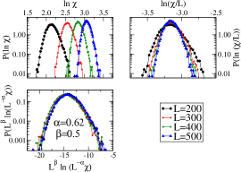
Figure 11: (color online) (a) Distribution $P(\ln\chi))$ at $\lambda=1.39$ for $L\in\{200,300,400,500\}$. (b) Distribution $P(\ln(\chi/L))$. (c) Rescaled distribution, $L^{\beta}\ln(L^{-\alpha}\chi)$. Here $\sigma=0.2$, $\gamma=1$, and the fit parameters are $\alpha=0.62$ and $\beta=0.5$. Including this exponential correction improves the collapse of the curves. This scaling would suggest $\chi\sim L^{\alpha}\exp{L^{-\beta}}$.

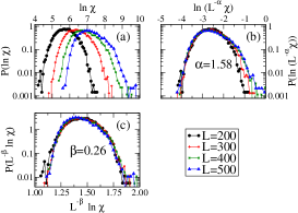
Figure 12: (color online) (a) Distribution $P(\ln\chi))$ at the pseudocritical point $\lambda=1.02$ for $L\in\{200,300,400,500\}$. (b) Distribution after a power-law rescaling $\ln(L^{-\alpha}\chi)$, where $\alpha=1.58$. (c) Distribution of $L^{-\beta}\ln\chi$ for $\beta=0.26$ and the same parameters. Here $\sigma=0.2$ and $\gamma=1$, though this collapse applies for all other disorder strengths considered.

III.2.2 Near the anisotropy line

Just like for the Ising case, far from the anisotropy line the distribution $P(\chi)$ is well-approximated as a Gaussian. Closer to the $\gamma=0$ line the distribution looks much like the distribution of $\ln\chi(\lambda)$ in the vicinity of the Ising line, becoming non-Gaussian with a slowly-decaying tail towards large values of $\chi$. Fig.(13) shows the distribution $P(\ln(\chi))$ for $\gamma=0$ and noise strength $\sigma=0.3$, and Fig.(14) shows the same quantity for $\gamma=0.03$, the value of average anisotropy coinciding with the peak in the typical value of $\chi$ for that magnitude of disorder.

Considering the point $\gamma=0$, as the system size increases the distribution $P(\ln\chi)$ does not change width, so a rescaling $\chi\to\chi/L$ gives a good collapse, see Fig.(15). This scaling also agrees with the extensive scaling of the average fidelity susceptibility at $\gamma=0$. Moving $\gamma$ away from this point in either direction, soon the distribution begins to shift superextensively, as shown in Fig.(16). For all values of $\gamma$ in this peak region, a rescaling of the form $\chi\to\chi/L^{\alpha}$ gives a good collapse, where $\alpha$ is the fit value of the finite-size scaling dimension of the corresponding typical fidelity susceptibility. Continuing to move $\gamma$ away from the peak in the typical fidelity susceptibility, the distribution begins to narrow slightly as in the off-critical Ising case. However, a rescaling $\chi\to\chi/L$ appears to give a good collapse for $\gamma$ sufficiently large in magnitude.

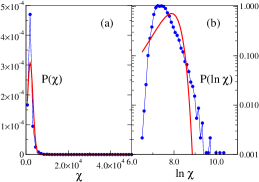
Figure 13: (color online) (a) Distribution of $\chi$ at the anisotropy line $\gamma=0$ (blue). Overlaid is a Gaussian distribution function with the same mean and variance (red). (b) Distribution of $\ln\chi$ for the same parameters (blue) along with the corresponding distribution function of the logarithm of a Gaussian random variable. Here $\sigma=0.3$, $L=500$, and $\lambda=0.5$. The distribution is non-Gaussian with a power-law tail towards large fidelity susceptibilities.

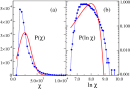
Figure 14: (color online) (a) Distribution for $\gamma=0.03$ (near the value of $\gamma$ coinciding with the peak in $\left[\chi\right]_{typ}$) (blue). Overlaid is a Gaussian distribution function with the same mean and variance (red). (b) Distribution of $\ln\chi$ for the same parameters (blue) along with the corresponding distribution function of the logarithm of a Gaussian random variable. Here $\sigma=0.3$, $L=500$, and $\lambda=0.5$. Note that there does not appear to be a power-law tail towards large fidelity susceptibilities.

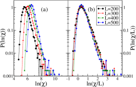
Figure 15: (color online) (a) Distribution $P(\ln\chi))$ at $\gamma=0$ for $L\in\{200,300,400,500\}$. (b) Rescaled distribution, $\ln(\chi/L)$ for the same parameters. Here $\sigma=0.3$ and $\lambda=0.5$, though this collapse applies for all other disorder strengths considered.

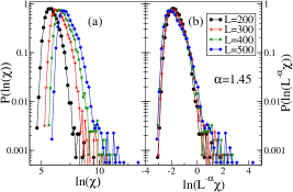
Figure 16: (color online) (a) Distribution $P(\ln\chi))$ at $\gamma=0.06$, the position of the maximum of $\left[\chi\right]_{typ}$ for $\sigma=0.3$. System sizes $L\in\{200,300,400,500\}$ are plotted. (b) Rescaled distribution, $\ln(L^{-\alpha}\chi)$ for the same parameters, with $\alpha=1.45$. Here $\sigma=0.3$ and $\lambda=0.5$.

IV Conclusion

In this work we have studied the effect of random transverse fields and couplings on the phase diagram of the quantum XY chain. By examining the finite-size scaling of the typical fidelity susceptibility and the fidelity susceptibility distribution for a range of disorder strengths and system sizes, we find agreement with earlier analytic results pertaining to the limit of weak randomness. The introduction of disorder clearly removes the anisotropy quantum critical line, replacing it with an extended Griffiths phase. There, the typical fidelity susceptibility’s finite-size scaling dimension depends strongly on the average value of the anisotropy parameter, and appears to become extensive at the line of vanishing anisotropy. At the Ising critical line, the stretched exponential scaling of the fidelity susceptibility distribution is consistent with what is expected of an infinite randomness fixed point, while a Griffiths phase is observed to form in the vicinity. Remarkably, the scaling of the fidelity susceptibility distribution at the Ising critical line is universal, in that all disorder strengths give the same scaling behavior. In the Griffiths phase the fidelity susceptibility is not self-averaging. However, self-averaging behavior returns sufficiently far from the disorder-free critical lines. These detailed results suggest that the fidelity susceptibility may be a useful tool for the study of other disordered systems.

We would like to thank N. Bray-Ali for helpful comments. Computation for the work described in this paper was supported by the University of Southern California Center for High Performance Computing and Communications. We acknowledge financial support by the National Science Foundation under grant DMR-0804914.

V Appendix

Here we derive an expression for the fidelity susceptibility $\chi$ in terms of the unitary matrix $T$:

$$F(Z,\tilde{Z})=\sqrt{|\det{\frac{T+\tilde{T}}{2}}|}$$ (7)

$$= \exp\left\{\textrm{Tr}\ln{\left(\frac{1+T^{\dagger}\tilde{T}}{2}\right)^{1/2}}\right\}$$

$$= \exp\left\{\textrm{Tr}\ln{\left(\frac{1+T^{\dagger}\left(T+\delta T\right)}{2}\right)^{1/2}}\right\}$$

$$= \exp\left\{\textrm{Tr}\ln{\left(1+\frac{T^{\dagger}\delta T}{2}\right)^{1/2}}\right\}$$

$$= \exp\left\{\textrm{Tr}\frac{1}{2}\ln{\left(1+\frac{T^{\dagger}\delta T}{2}\right)}\right\}$$

$$\approx \exp\left\{\textrm{Tr}\frac{1}{2}\left[\frac{1}{2}T^{\dagger}\delta T-\frac{1}{8}\left(T^{\dagger}\delta T\right)^{2}\right]\right\},$$

where $\delta T=\partial_{x}Tdx$. This leads to

$$F(Z,\tilde{Z})=\exp\left\{\textrm{Tr}\frac{1}{2}\left[\frac{1}{4}T^{\dagger}\partial_{x}^{2}Tdx^{2}-\frac{1}{8}T^{\dagger}\partial_{x}TT^{\dagger}\partial_{x}Tdx^{2}\right]\right\}$$ (8)

$$= \exp\left\{-\frac{1}{8}\|\partial_{x}T\|_{F}^{2}dx^{2}-\frac{1}{16}\textrm{Tr}\left[T^{\dagger}\partial_{x}TT^{\dagger}\partial_{x}T\right]dx^{2}\right\}$$

$$= \exp\left\{-\frac{1}{8}\|\partial_{x}T\|_{F}^{2}dx^{2}-\frac{1}{16}\textrm{Tr}\left[-\partial_{x}T^{\dagger}TT^{\dagger}\partial_{x}T\right]dx^{2}\right\}$$

$$= \exp\left\{-\frac{1}{8}\|\partial_{x}T\|_{F}^{2}dx^{2}-\frac{1}{16}\textrm{Tr}\left[-\partial_{x}T^{\dagger}\partial_{x}T\right]dx^{2}\right\}$$

$$= \exp\left\{-\frac{1}{16}\|\partial_{x}T\|_{F}^{2}dx^{2}\right\},$$

where we have used the anti-symmetry of $T^{\dagger}\partial_{x}T$ which implies $\textrm{Tr}\left[T^{-1}\partial_{x}^{2}T\right]=-\|\partial_{x}T\|_{F}^{2}$, with $\|\cdot\|_{F}$ the Frobenius norm. From (4) it follows that

$$\chi=\frac{1}{8}\|\partial_{x}T\|_{F}^{2}.$$ (9)

References

- (1) P. Zanardi and N. Paunković, Phys. Rev. E 74, 031123 (2006)
- (2) H.Q. Zhou and J.P. Barjaktarevic, arXiv:cond-mat/0701608
- (3) H.Q. Zhou, J.H. Zhao and B. Li, arXiv:0704.2940
- (4) H.Q. Zhou, arXiv:0704.2945
- (5) S.J. Gu, arXiv:0811.3127v1
- (6) P. Zanardi, H.T. Quan, X. Wang, and C.P. Sun, Phys. Rev. A 75, 032109 (2007)
- (7) P. Zanardi, L. Campos Venuti, P. Giorda, Phys. Rev. A 76, 062318 (2007)
- (8) H. T. Quan, F. M. Cucchietti, Phys. Rev. E 79, 031101 (2009)
- (9) A. Hamma, W. Zhang, S. Haas and D.A. Lidar, Phys. Rev. B 77, 155111 (2008)
- (10) D.F. Abasto, P. Zanardi, Phys. Rev. A 79, 012321 (2009)
- (11) D.F. Abasto, A. Hamma, P. Zanardi, Phys. Rev. A 78, 010301(R) (2008)
- (12) S. Yang, S.J. Gu, C.P. Sun and H.Q. Lin, Phys. Rev. A, 78, 012304 (2008)
- (13) S. Garnerone, D.F. Abasto, S. Haas, and P. Zanardi, Phys. Rev. A 79, 032302 (2009)
- (14) Erik Eriksson and Henrik Johannesson, arXiv:0902.3848
- (15) S. Garnerone, N.T. Jacobson, S. Haas, and P. Zanardi, Phys. Rev. Lett., 102, 057205 (2009).
- (16) F. Igloi and C. Monthus, Phys. Rep. 412 277 (2005)
- (17) R.B. Griffiths, Phys. Rev. Lett 23, 17 (1969)
- (18) E. Lieb, T. Schultz and D. Mattis, Ann.Phys. 16, 407 (1961)
- (19) R.H. McKenzie, Phys. Rev. Lett. 77, 4804 (1996)
- (20) J.E. Bunder, R.H. McKenzie, Phys. Rev. B 60, 344 (1999)
- (21) M. Cozzini, P. Giorda, P. Zanardi, Phys. Rev. B 75, 014439 (2007)
- (22) P. Zanardi, M. Cozzini, P. Giorda, J. Stat. Mech. (2007) L02002
- (23) W.L. You, Y.W. Li, S.J. Gu, Phys. Rev. E 76, 022101 (2007)
- (24) L. Campos Venuti and P. Zanardi, Phys. Rev. Lett. 99, 095701 (2007)
- (25) C. Dasgupta and S.K. Ma, Phys. Rev. B 22, 1305 (1980)
- (26) D.S. Fisher, Phys. Rev. Lett. 69, 534 (1992)
- (27) D.S. Fisher, Phys. Rev. B 51, 6411 (1995)
- (28) A.P. Young and H. Rieger, Phys. Rev. B 53, 8486 (1996)
- (29) A. Aharony and A.B. Harris, Phys. Rev. Lett. 77, 3700 (1996)