Membership and lithium in the old, metal–poor open cluster Berkeley 32

Abstract

Context. Measurements of lithium (Li) abundances in open clusters provide a unique tool for following the evolution of this element with age, metallicity, and stellar mass. In spite of the plethora of Li data already available, the behavior of Li in solar–type stars has so far been poorly understood.

Aims. Using FLAMES/Giraffe on the VLT, we obtained spectra of 157 candidate members of the old, metal–poor cluster Berkeley 32, to determine membership and to study the Li behavior of confirmed members.

Methods. Radial velocities were measured, allowing us to derive both the cluster velocity and membership information for the sample stars. The Li abundances were obtained from the equivalent width of the Li i 670.8 nm feature, using curves of growth.

Results. We obtained an average radial velocity of $105.2\pm 0.86$ km/s, and 53 % of the stars have a radial velocity consistent with membership. The Li – T_eff distribution of unevolved members matches the upper envelope of M 67, as well as that of the slightly older and more metal-rich NGC 188. No major dispersion in Li is detected. When considering the Li distribution as a function of mass, however, Be 32 members with solar-like temperature are less massive and less Li-depleted than their counterparts in the other clusters. The mean Li of stars in the temperature interval $5750\leq\rm T_{\rm eff}\leq 6050$ K is $\log$ n(Li)=$2.47\pm 0.16$, less than a factor of two below the average Li of the 600 Myr old Hyades, and slightly above the average of intermediate age (1–2 Gyr) clusters, the upper envelope of M67, and NGC 188. This value is comparable to or slightly higher than the plateau of Pop. ii stars. The similarity of the average Li abundance of clusters of different age and metallicity, along with its closeness to the halo dwarf plateau, is very intriguing and suggests that, whatever the initial Li abundance and the Li depletion histories, old stars converge to almost the same final Li abundance.

1 Introduction

Despite its low abundance (N(Li)/N(H) $\leq 2\times 10^{-9}$), lithium (Li) plays a fundamental role in different fields of astrophysics because of how it is created and destroyed. The ⁷Li isotope is the heaviest element produced during Big Bang nucleosynthesis (BBN), and its primordial abundance strongly depends on $\eta$, the ratio of baryons to photons (e.g., Steigman steig_cast (2006) and references therein). At the same time, Li is easily depleted from stellar atmospheres: ⁷Li is destroyed by proton reactions at the relatively low temperature of $\sim 2.5$ MK, implying depletion with respect to the initial content whenever a mixing process is present that is able to transport surface material down to the deeper regions in the stellar interior where this temperature is reached.

Primordial Li abundance has been empirically estimated by means of Li measurements in old Pop. ii stars and, theoretically, using BBN calculations combined with the baryon density derived from measurements of the cosmic microwave background temperature fluctuations. The reliability of the latter has dramatically improved after data from the WMAP satellite became available (Cyburt et al. cyburt (2003); Spergel et al. spergel (2007)). Estimates from old stars rely on the assumption that the hot (T${}_{\rm eff}\geq$ 5800 K), metal poor, Pop. ii dwarfs do not deplete Li in their atmosphere, hence represent the primordial material from which they were born. The confidence on this assumption is based on the near constancy of their Li abundance with metallicity, first discovered by Spite & Spite (spite82 (1982)) and generally referred to as the Spite plateau. Primordial Li abundance predicted from standard BBN calculations with WMAP is a factor of two to three higher than that of the Spite plateau, which might indicate that halo stars have indeed undergone some Li depletion, possibly due to microscopic diffusion, as recently claimed by Korn et al. (korn (2006), korn1 (2007)). Only through a full understanding of mixing inside stars and its dependence on metallicity will we be able to reach a conclusion with complete confidence.

To achieve that, studies in Pop. i stars, and in particular among open cluster members, are the most suitable observation tool. Lithium (and beryllium) measurements in Galactic open clusters (OCs) indeed allow us to empirically trace Li depletion with age, metallicity, and mass. Focusing on solar-type stars, standard models of stellar evolution (those including convection only) predict that these stars should not suffer any Li depletion during the main sequence (MS), since their convective zone does not reach the Li burning layer. Surveys of Li in a variety of OCs and, in particular, the comparison of the Li patterns of OCs of different age, have shown that, at variance with these predictions, solar-type stars do deplete Li on the MS. Depletion starts at $\sim 100$ Myr and smoothly goes on up to the Hyades age, on a timescale of $\sim 1.4$ Gyr. After that age depletion becomes bimodal: it is very fast for a fraction of stars, like the Sun itself, and the lower envelope of M 67 (Pasquini et al. pas97 (1997) and references therein), while depletion completely stops after $\sim 1$ Gyr for a significant fraction of stars (Sestito & Randich sr05 (2005); Prisinzano & Randich pr07 (2007)) In particular, Randich et al. (randich_188 (2003) -RSP03 hereafter) have shown that members of the old (6–8 Gyr) OC NGC 188 have a Li abundance only a factor of two smaller than their counterparts in the factor of 10 younger Hyades; moreover, the average value of Li in NGC 188 is surprisingly close to what is measured in Pop. ii stars. This open cluster has a solar metallicity and, as discussed by RSP03, this result might be a mere coincidence; however, the issue is obviously worth further studies. It might indeed represent a link between Pop. i and Pop. ii. Li depletion histories and provide a clue to understand whether the latter have undergone Li depletion. Investigating Li in additional very old OCs is thus very important.

It is worth mentioning that, to explain the unexpected Li depletion during the MS, several non-standard processes were included in the models. The proposed mechanisms include diffusion (Michaud mich86 (1986), Michaud et al. mich04 (2004); Chaboyer et al. chab95 (1995)), meridional circulation (Charbonnel & Talon ct99 (1999) and references therein), angular momentum loss and rotationally driven mixing (Eddington 1925; Zahn 1974, 1992; Deliyannis & Pinsonneault 1997), gravity waves (García López & Spruit 1991; Montalbàn & Schatzmann 2000), tachocline (Spergel & Zahn 1992; Brun et al. 1999; Piau et al. 2003), and combinations of waves and rotation (Charbonnel & Talon ct05 (2005); Talon talon (2008)). Each of these models makes specific predictions on the timescales of Li depletion which can be compared with observational patterns.

We present here Li observations in a very large sample of members of Berkeley 32. This open cluster is one of the oldest in the Galaxy (5 Gyr –e.g. D’ Orazi et al. dorazi (2006)) and its metallicity is a factor of two below solar (Sestito et al. sestito06 (2006)); therefore, it provides an ideal sample to further investigate the issue of the convergence of Li at old ages.

The paper is organized as follows. In Sect. 2 we describe the sample, the observations, and data reduction. Data analysis and the results are presented in Sects. 3 and 4. A discussion is provided in Sect. 5, followed by conclusions in Sect. 6.

2 Sample and observations

The observations were obtained with VLT/FLAMES. Specifically, we used the fiber link to UVES to acquire spectra of evolved stars (RGB and clump stars) to be used for the determination of the cluster chemical compositions (Sestito et al. sestito06 (2006); Bragaglia et al. brag08 (2008)), while the Giraffe spectrograph and Medusa fiber system were employed to observe MS and/or turn-off (TO) cluster candidates as well as a few subgiants, in order to derive membership and information on Li.

2.1 Targets

Photometric surveys of Be 32 have been performed by Kaluzny & Mazur (km91 (1991)), Richtler & Sagar (rs00 (2000)), Hasegawa et al. (hase (2004)), and D’ Orazi et al. (dorazi (2006)). A re-analysis of D’ Orazi et al. photometry was performed by Tosi et al.(tbc (2007)). All these studies agree on a cluster age of 5–6 Gyr, on a subsolar metallicity, and on a reddening E(B–V) in the range 0.08 – 0.16, with a most likely value of 0.1–0.12 (see discussion in Tosi et al.). Based on UVES spectra of nine cluster members Sestito et a. (sestito06 (2006)) derived for the cluster a metallicity [Fe/H]=$-0.29\pm 0.04$. So far no spectroscopic studies of MS stars have been performed and membership is based only on photometric criteria.

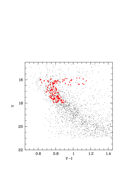
Figure 1: V vs. V–I diagram of Be 32 with FLAMES targets shown as filled symbols. The whole catalog was constructed using Richtler & Sagar (rs00 (2000)) photometry. We show in the figure only stars brighter than V=21.

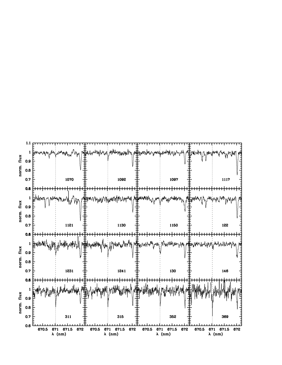
Figure 2: Sample spectra in the Li region. The position of the Li line is marked.

We selected Giraffe target stars from the catalogs of Kaluzny & Mazur (km91 (1991)) and Richtler & Sagar (rs00 (2000)), since the study of D’Orazi et al. was still in preparation at the time of the observations. The V – V–I diagram of the target stars is displayed in Fig. 1 which shows that the sample includes stars from the cluster subgiant branch and turn-off (TO) (V $\sim 16$) down to V=18. As mentioned, membership for these candidates so far has been based only on photometry. One of the purposes of this study is a more reliable determination of membership via radial velocity measurements.

2.2 Observations and data reduction

Be 32 was observed with two different FLAMES configurations (A and B) centered at RA(2000)=06h 58m 04.2s and DEC(2000)=$-$06d 28m 21.1s and RA(2000)=06h 58m 02.0s and DEC(2000)=$-$06d 22m 41.4s, respectively. We obtained four and one 3600 s long exposures for configurations A and B, respectively. Observations were obtained in Visitor mode on Jan. 20, 2005 (configuration A) and Jan. 21, 2005 (configuration B). Medusa fibers were allocated to 112 and 108 objects in the two configurations, with 63 stars in common. In total we thus obtained spectra of 157 cluster candidates. In both configurations 15 fibers were put on the sky. Stars covered by configurations A and B were observed for a total of 4 and 1 hrs, respectively, while the 63 stars in common were observed for 5 hrs. Target stars, together with their photometry, are listed in Table Membership and lithium in the old, metal–poor open cluster Berkeley 32 . In the table we list our running ID (Col. 1), coordinates from Kaluzny & Mazur (km91 (1991)) if the star is present in their catalog otherwise from Richtler & Sagar (rs00 (2000) –Cols. 2-3); photometry from D’ Orazi et al. (dorazi (2006) –Cols. 4–7); V magnitude from Kaluzny & Mazur (km91 (1991)) if the star is present in their catalog otherwise from Richtler & Sagar (rs00 (2000) –Col. 8); B–V from Kaluzny & Mazur (Col. 9); V–I from Richtler & Sagar (Col. 10); radial velocity and membership flag (Cols. 11–12). Giraffe was used in conjunction with the 316 lines/mm grating and order- sorting filter 15 (H15N) yielding a nominal resolving power R=17000 and covering a spectral interval from 644.2 to 681.8 nm, including the Li i 670.8 nm line and several features to be used for radial velocity measurements.

Data reduction was performed using the Giraffe BLDRS pipeline, following the standard procedure and steps (Blecha et al. blecha04 (2004)). Sky subtraction was carried out separately; namely, we first computed the average sky (sky_av.) of three sets of five sky spectra and then derived the median of the three sky_av.. Radial velocities (RV) were derived from each single spectrum (see below). Spectra of stars that were not found to be RV variables were then co-added. Examples of final, sky-subtracted spectra are shown in Fig. 2. Final S/N range between 20 and 85, with an average value of $\sim 50$.

3 Analysis

3.1 Radial velocities

Radial velocities were obtained from our spectra and used to derive membership information for the sample stars. The 645 - 682  nm region contains a large number of unblended lines (mainly Fe, Ca, Ti, and Ni) of various strengths suitable for accurate RV measurements. The individual lines used for the RV computation are listed in Table 2.

Figure 3: Density distribution of radial velocities for the 153 stars for which we could get a measurement. The two Gaussians (solid curves) indicate the best fits for the cluster and field, respectively. The average velocities along with $1\sigma$ dispersion are indicated.

Table 2: Individual lines suitable for RV computations.

line & multiplet	$\lambda$ (Å)
CaI 19	6449.810
CaI 18	6462.566
CaI 18	6471.660
FeI 206	6475.632
FeI 168	6494.985
FeI 268 + Ti 102	6546.252
Hα	6562.808
FeI 268	6592.926
FeI 1197	6633.764
NiI 43	6643.641
FeI 111	6663.446
FeI 268	6677.993
LiI 1	6707.815
CaI 32	6717.687
FeI 111	6750.152
NiI 57	6767.778
FeI 205	6783.710
FeI 268	6806.851
FeI 1197	6810.280

The data analysis was performed by standard procedures within the IRAF package, fitting the strongest lines present in each spectrum by a Gaussian profile. The resulting RVs from the individual lines were averaged, and heliocentric corrections applied. Normally less than ten lines per spectrum allowed us to obtain an RV value with an error of about 2 km/s; RV values of spectra referring to the same star were then averaged for stars in configuration A having multiple exposures. Final radial velocities with their errors are given in Col. 9 of Table  Membership and lithium in the old, metal–poor open cluster Berkeley 32 . For stars with multiple RV measurements, the error is the standard deviation from the average RV, while for stars in configuration B the error is the uncertainty in the RV measurement itself.

3.2 Li abundances

Lithium abundances were derived by measuring the equivalent width (EW) of the Li I line at 670.8 nm. Measurements were performed by direct integration below the continuum. For stars with detected Li, each measurement was performed twice, meaning we determined the maximum and minimum reasonable values. We then adopted the average between these two last values as EW measurement, and we used half of the difference between them as the error estimate on EW. In some RV members, the Li line could not be detected and we measured its upper limit, which was estimated as the EW of the smallest detectable feature in the Li spectral region. We measured the Li line in both radial velocity members and non-members. Whereas for most radial velocity members we detected the Li line, for six and 19 stars in fields A and B the S/N was too low to even infer a meaningful upper limit. We mention in passing that these stars are not necessarily fainter than those where the Li line was measurable. Lithium was also detected in 27 RV non-members.

Effective temperatures were determined on the basis of published photometry (Richtler & Sagar rs00 (2000); D’Orazi et al. dorazi (2006)) and using the color versus temperature calibrations by Alonso et al.  (al96 (1996) –for MS stars, al99 (1999) –for evolved stars). When available, we used the photometry of D’Orazi et al., while we took colors from Richtler & Sagar for stars not included in the study of D’ Orazi et al. As shown by Tosi et al. (tbc (2007)), the agreement between the two photometries is very good for most stars in the magnitude range considered here. More specifically, we used B–V colors from D’ Orazi et al. (dorazi (2006)) for 45 stars out of the 47 for which they were available. Stars #364 and #1241 have B–V colors from D’Orazi et al., but that of the former star is too red compared to the V–I, while B–V of the latter is much bluer than the cluster sequence on the CM diagram; therefore we did not use B–V from D’Orazi et al. We employed B–V of Kaluzny & Mazur (km91 (1991)) for two stars not included in the study of D’Orazi et al. (#236 and #333) and for the aforementioned star #364. Finally, for star #1241 and for eight stars without available B–V we transformed V–I into B–V using a linear relationship that nicely fits the sequence of stars with both colors available. Reddening determinations towards Be 32 vary between E(B–V)=0.10 and 0.18 mag (see Tosi et al. tbc (2007)); we assumed the value E(B–V)$=0.14$, determined by Bragaglia et al. (brag08 (2008)) using spectroscopic temperatures, since we regard it as more reliable than values obtained from main sequence fitting.

To evaluate the random error that affects our temperature determinations, we compared effective temperatures based on the B–V colors of D’ Orazi et al. with those estimated from B–V of Kaluzny & Mazur for the 32 stars studied in both referenced papers. The average $\Delta$T_eff =(T_eff${}^{\rm D^{\prime}Orazi}$-T_eff^K&M) is $-50$ K with a standard deviation equal to 116 K. We adopt this value as the typical error on effective temperatures.

In previous studies (see Sestito& Randich sr05 (2005)), we derived effective temperatures using the calibration of Soderblom et al. (1993a ). Since this calibration does not have a term taking into account metallicity, we prefer to use Alonso’s calibrations for Be 32, whose metallicity is below solar. Soderblom et al.’s calibration would have given warmer temperatures, with a typical difference of 144 K. However, at solar metallicity the two scales are very similar.

As is well known, at our resolution the Li line is blended with a Fe i line. To estimate the contribution of Fe to the total EW, we cannot use the analytical approximation of Soderblom et al. (1993b ), which was derived using stars with solar metallicity. We instead estimated the EW of this feature employing MOOG (Sneden sneden (1973) –Version 2000) and the driver ewfind using the appropriate metallicity and stellar parameters. Effective temperatures were derived as described above. The surface gravity for evolved stars was estimated in the same fashion as in Sestito et al. (sestito06 (2006)), while for stars on the MS we assumed $\log$ g=4.5. Microturbulence values $\xi=1.1$ and 1.5 km/s were used for unevolved and evolved stars, respectively. We found that for MS objects EW(Fe 6707.44)=$(22.5-3.3\times 10^{-3}\times\rm T_{\rm eff}$) Å, while the EW of the Fe line was computed separately for each evolved star. The strength of this shallow Fe line has a very weak dependence on both the microturbulence $\xi$ and $\log$ g: a change in $\xi$ of 1 km/s results in a change in EW below 0.2 mÅ, while a change of 0.5 dex in $\log$ g results in a difference of $\sim 0.2$ mÅ.

The Li abundances were derived from corrected EWs using Soderblom et al. (1993b ) curves of growth (COGs), which assume local thermodynamic equilibrium (LTE). A correction for non–LTE effects following Carlsson et al. (carls (1994)) has also been run on our data, but it produces no significant changes. Li for evolved stars was instead derived using MOOG, which allows changing surface gravity and microturbulence. Using of a different code and method to derive Li for evolved and unevolved stars introduces a small offset between the two abundance scales. By using MOOG, we would obtain slightly higher $\log$ n(Li) for dwarf stars, typically by 0.05-0.1 dex. On the one hand, this offset does not affect our results and, in particular, our conclusions on dilution in more evolved stars (Figs. 5 and 6); on the other hand, the use for Be 32 dwarf members of the same COGs employed in the literature for other OCs is critical to correctly draw the time evolution of Li.

The final error on the Li abundance measurement is computed by summing quadratically the contributions from EW and temperature. Errors in the Fe I contribution due to errors in T_eff are very small, much smaller than the errors in the EW measurements themselves: namely, $\delta$EW(Fe I)=0.5 mÅ for $\delta$T_eff=100 K.

4 Results

4.1 Radial velocities and membership

In Fig. 3, we show the density distribution of radial velocities for the 153 stars for which we were able to measure them. The figure clearly shows a very narrow peak that indicates the presence of the cluster. To derive the average cluster radial velocity, we fitted the observed distribution with two Gaussians, one for the cluster and one for the field, and determined the best fit using a maximum likelihood algorithm. We obtained RV${}_{\rm cluster}=105.2$ Km/s, $\sigma_{\rm cluster}=0.86$ Km/s and RV${}_{\rm field}=62.6$ Km/s, $\sigma_{\rm field}=32.1$ Km/s, respectively. Our measurement of the RV is in good agreement with the values of D’ Orazi et al. (dorazi (2006), RV=106.7$\pm 8.5$ Km/s) from low- resolution spectroscopy of 48 stars brighter than the turn-off, of Sestito et al. (sestito06 (2006), RV=106$\pm 1.4$ Km/s), and of Scott, Friel, & Janes (scott (1995), 106$\pm 10$ Km/s) from the intermediate-resolution spectroscopy of 10 giants. Also, three stars in our sample have an RV measurement from D’Orazi et al.: #74 (their #698), #97 (their #113), and #1090 (their #364). The agreement in RV is excellent for all of them. We stress that, thanks to our large sample, we have been able to constrain the internal dispersion in velocity much better than in previous studies, pushing it to below 1 Km/s.

We considered all stars as cluster members with RV within $3\sigma$ from the cluster average: adopting this criterion, 59 and 24 stars turned out to be members in fields A and B. The total fraction of members is 83/153 stars, i.e., 54 %. The expected number of contaminants, or non members with RV consistent with the cluster, is 2 stars. Since our observations were obtained within the same night, we have only been able to identify one possible binary systems (star #1090). This system has average velocity consistent with membership, but a double-line system and larger-than-average deviation around the mean. We have tentatively classified it as an SB2 cluster member. Most likely, additional unidentified binaries might be present among stars with RV discrepant with membership and detected Li line. Further follow-up is needed to confirm their membership. Therefore, we regard the fraction of members as a lower limit to the real value.

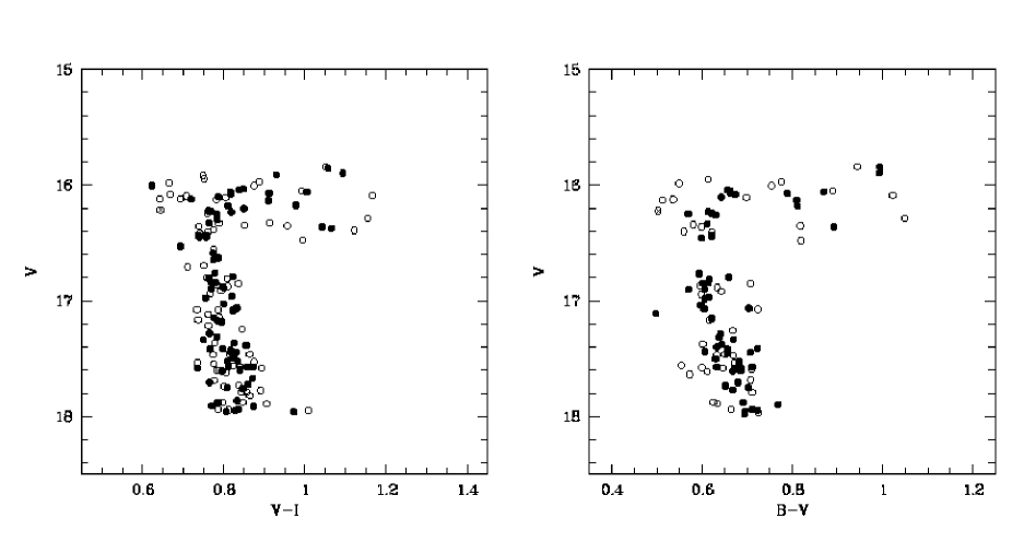
Figure 4: “Cleaned” color-magnitude diagrams. Open symbols represent all observed stars, while filled symbols denote radial velocity members. The crossed symbol denotes the possible SB2 binary. When available we have considered photometry from D’Orazi et al. (dorazi (2006)), while in the other cases we have considered B–V colors from Kaluzny & Mazur (km91 (1991)) and V–I colors from Richtler & Sagar (rs00 (2000)).

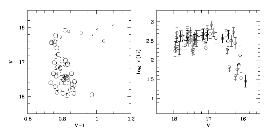
Figure 5: Panel a) V – V–I diagram of confirmed cluster members. Different symbol sizes indicate different Li abundance bins; namely, from the largest to the smallest ones: $\log$ n(Li)$\geq 2.0$, 2.0$\leq$ $\log$ n(Li)$<1.7$, and $\log$ n(Li)$<1.7$. For 47 of the 57 stars with a Li measurement, we have considered photometry from D’Orazi et al. (dorazi (2006)), while for the remaining 10 stars not included in the D’Orazi et al. study, we used Richtler & Sagar (rs00 (2000)) magnitudes and colors. Panel b): Lithium abundance –$\log$ n(Li), in the usual logarithmic scale where n(H)=12– as a function of V magnitude for confirmed cluster members.

The “cleaned” CM diagrams are shown in Fig. 4, where RV members and non-members and the SB2 binary are denoted with different symbols. Whereas we refer to Tosi et al. (tbc (2007)) for a detailed discussion of the analysis of the cluster CM diagram, we mention here that our membership determination has allowed us to clean the turn-off region, thus allowing a more solid derivation of cluster parameters, as done by Tosi et al. Among the subgiants we note the presence of two confirmed members (one in the V vs. B–V diagram) somewhat fainter than the cluster sequence. We do not have any explanation for them, but suggest that they might be the two expected contaminants.

4.2 Lithium abundances

In Table References we list confirmed members (from Table Membership and lithium in the old, metal–poor open cluster Berkeley 32 ) for which we were able to either measure the EW of the Li line or infer a reasonable upper limit. In the table we provide IDs (same as in Table  Membership and lithium in the old, metal–poor open cluster Berkeley 32 ), dereddened B–V colors, effective temperatures, measured Li equivalent widths, and Li abundances. The last are in the usual notation $\log$ n(Li)=$\log$N(Li)/N(H)+12. In Fig. 5a we plot the V–V$-$I diagram of cluster members with different symbol sizes denoting stars with different Li contents, while in Fig 5b we show Li abundances as a function of V magnitude. The figures very well illustrate the evolution of Li along the CM diagram. All stars on the MS and at the TO have Li abundances larger than $\log$ n(Li)$=2$ and their present Li abundance is the result of MS depletion; on the other hand, cluster members slightly more evolved than TO have started diluting their surface Li, due to the deepening of the convective zone (e.g., Randich et. al. randich_subg (1999)). The transition between stars that have and that have not undergone dilution occurs in a very narrow magnitude range (see also Pasquini et al. pas04 (2004)). Dilution progressively continues along the subgiant branch, up to a Li abundance $\sim 1$.

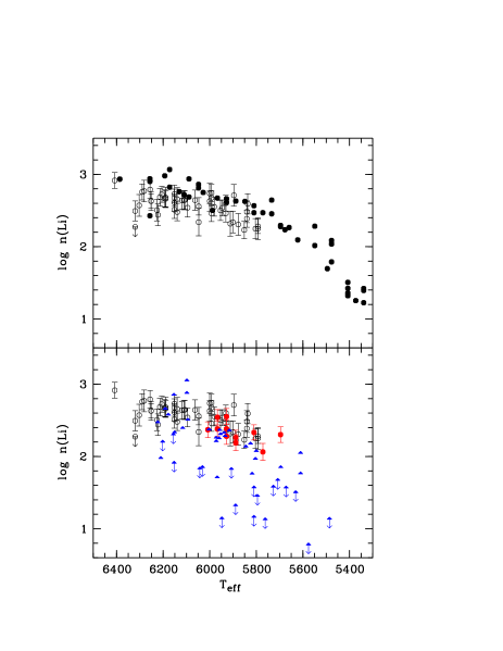
Figure 6: Upper panel: comparison of the distribution of $\log$ n(Li) as a function of T_eff for unevolved stars in Be 32 (open circles) and the Hyades (filled circles); lower panel: same as upper panel, but Be 32 is compared to M67 (filled triangles) and NGC 188 (filled circles).

In Fig. 6 we show the usual plot of Li abundances as a function of effective temperature for unevolved cluster stars (TO and MS) and compare Be 32 with the much younger and more metal-rich Hyades (upper panel) and with both the slightly younger M 67 and the slightly older cluster NGC 188 (lower panel). Both NGC 188 and M 67 OCs have a solar metallicity (Randich et al. randich_188 (2003), randich_m67 (2006)), and thus are a factor of $\sim 2$ more metal rich than Be 32. Lithium abundances for the three OCs were taken from the compilation of Sestito & Randich (sr05 (2005)). In that paper Li abundances had been derived using the same COGs and NLTE correction employed here.

The figure shows that, at variance with the Hyades and M 67, but more like NGC 188, Be 32 distribution does not show any major trend of decreasing Li abundance with decreasing T_eff. We find average Li abundance values of $\log$ n(Li)$=2.63\pm 0.17,2.62\pm 0.07$, and $2.47\pm 0.16$ for stars in the temperature ranges T_eff $>6200$ K, 6200$\geq$T_eff$\geq 6000$  K, and T_eff$<$6000 K. The three average values are, within the errors, the same. Also, at variance with M 67, but similar to NGC 188, the Be 32 sample is not characterized by any significant (larger than errors) dispersion in Li. More specifically, Figs. 5b and 6 show that the maximum star-to-star difference for unevolved stars is on the order of 0.5 dex. Assuming Gaussian statistics, this corresponds to a 1$\sigma$ dispersion of $\sim 0.15$ dex, comparable to the average error in $\log$ n(Li). Given the large size of our sample, we regard the lack of a significant scatter as real and not due to low number statistics and conclude that the appearance of the spread among open cluster stars is an exception rather than the rule, since the majority of OCs do not show it. Most important, whereas Hyades stars warmer than $\sim 6000$ K are somewhat more Li-rich than their Be 32 counterparts, the Li distributions of cooler stars are almost indistinguishable. The $\log$ n(Li)–T_eff of NGC 188 and Be 32 patterns are also very similar and close to the upper envelope of M67. In other words, the comparison of OCs of different ages and metallicity shows that, with the exceptions of the severely Li-depleted stars in the lower envelope of M 67, stars in the $\sim 6000-5700$ K T_eff range seem to converge to a very similar value of Li abundance.

5 Discussion

5.1 Pop. i plateau

The present study allows us to make firm conclusions about the empirical evolution of Li abundance during the MS of stars with temperatures (but not necessarily masses –see next section) similar to the Sun. In Fig. 7 we show the mean Li abundance as a function of age for stars in the 6050–5750 temperature range. The figure was done using the data of Sestito & Randich (sr05 (2005)), to which we added the average Li abundance of the $\sim$1 Gyr old NGC 3960 (from Prisinzano & Randich pr07 (2007)) and the average for Be 32 inferred here. As already discussed by Sestito & Randich, stars in this T_eff interval undergo a smooth, but continuous Li depletion during the first $\sim 600$ Myr on the main sequence, on a typical timescale of $\sim 1.4$ Gyr. As already mentioned, at older ages depletion becomes bimodal: it continues for a fraction of stars, while it stops for the majority of stars and the average $\log$ n(Li) converge to a plateau, which is quantitatively -and surprisingly- close to the plateau of Pop. ii stars. The evidence for this Pop. i plateau is statistically confirmed by the inclusion in the sample of the Be 32, for which we derived an average abundance $\log$ n(Li)=$2.47\pm 0.16$. This value is, slightly higher, but within the margins of error consistent, with that of the intermediate age OCs ($2.33\pm 0.17$), the upper envelope of M 67 ($2.25\pm 0.12$), and NGC 188 ($2.34\pm 0.14$). As to the Pop. ii plateau, values range between a minimum of $2.10\pm 0.09$ (Bonifacio et al. bon07 (2007)) and a maximum of $\sim 2.4$ (Meléndez & Ramirez mel04 (2004)).

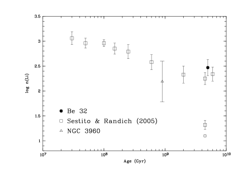
Figure 7: Average Li abundance as a function of age for stars in the 5750–6050 K interval. Open squares are OCs from Sestito and Randich (sr05 (2005)), the open triangle represents the average for NGC 3960 (Prisinzano & Randich (pr07 (2007)), while the filled circle denotes Be 32. For M 67 the average of the upper and lower envelopes are plotted. The Sun is also shown in the figure.

The conclusion is that Pop. I stars are not necessarily heavily Li-depleted, even at very old ages. The major consequence is that Li cannot be used as an age indicator for stars older than $\sim 500$ Myr: a lithium abundance in the interval $\log$ n(Li) $\sim 2.3-2.6$ does not allow discerning whether a star is 0.5 or 6 Gyr old. The above points are to be kept in mind when deriving the properties, age in particular, of stars hosting extra-solar planets. On the other hand, the Sun represents an exception and is not representative of Li depletion in solar–type stars, since it has undergone a larger-than-normal depletion. We believe that low Li (a factor greater than 30-50 depletion) should be regarded as indicative of a peculiar, but similar-to-the Sun, evolution.

5.2 Lithium as a function of stellar mass

Figure 6 clearly shows that the amount of Li depletion at a given T_eff does not depend on the cluster metallicity. The lack of any Li-metallicity dependence has already been discussed by Sestito & Randich (sr05 (2005)) on empirical grounds and by Piau et al. (piau (2003)) on theoretical grounds. The latter study show that metallicity variations on the order of 0.1 dex result in changes of both T_eff and temperature at the basis of the convective zone (T_BCZ); however, the relationship between T_eff and T_BCZ, and thus the amount of depletion at a given T_eff, remain almost unaltered. The inclusion of Be 32 in the open cluster sample and the comparison with the Hyades shows that this holds true for metallicity differences as large as 0.4-0.5 dex.

As is well known, however, metallicity does affect stellar structure: specifically, for a given mass, lower metallicities correspond to higher T_eff. In contrast, for a given effective temperature, lower metallicity stars have lower masses and stars with the same, close-to solar temperature, do not have the same, solar mass, if their metal content is different. In order to investigate Li depletion as a function of mass, we derived masses for unevolved stars in Be 32, as well as for the Hyades, M 67, and NGC 188 using the Padova isochrones (Girardi et al. girardi (2000) –http://pleiadi.pd.astro.it/) and the appropriate metallicities. When needed, we interpolated between different isochrones.

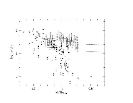
Figure 8: $\log$ n(Li) as a function of mass for Be 32 (open circles), the Hyades (asterisks), M 67 (filled triangles), and NGC 188 (filled circles). The horizontal lines delimits the range covered by Pop. II stars considering the lowest and highest values of the plateau.

In Fig. 8 we compare Li abundances as a function of mass for unevolved stars in Be 32 with the Hyades, M 67, and NGC 188 members. The range covered by Pop. II stars is also shown. This figure indicates that the distributions of the different OCs no longer overlap in the $\log$ n(Li)– mass diagram as it was instead the case for the $\log$ n(Li)–T_eff plane. This is due to the fact that Be 32 stars with temperatures close to solar are less massive than the Sun, of their counterparts in the solar metallicity NGC 188 and M 67, and of their metal-rich counterparts in the Hyades. The figure proves that Be 32 members at all masses have depleted less Li than stars with similar mass in the other old OCs; also, focusing on star with mass close to solar, the figure shows that NGC 188 members and the upper envelope of M 67 have depleted the same Li as their more metal-rich Hyades counterparts. In summary, both the timescales and the amount of Li depletion are different for stars with the same mass and different metallicities. This result indicates that, when looking at masses, metallicity affects the amount of depletion at a given age. In contrast, we stress again that the evolution of star with the same T_eff does not depend on [Fe/H] (at least within $\pm 0.2-0.3$ dex from the solar value), since more metal-poor and less massive stars, have the same internal structure of solar-metallicity, solar-mass ones.

5.3 Comparison with model predictions

For a formally correct comparison of the empirical evolution of Li with model predictions at a given mass, one should not mix data of OCs with significantly different metallicities or, alternatively, the appropriate metallicity should be considered. However, we believe that the comparison between model predictions and empirical evolution in a given temperature range can still be performed, since, at least as far as Li is concerned, the evolution of stars with similar temperatures, but different masses and metallicities is virtually the same. As an example, we show again in Fig. 9 the mean Li abundance as a function of age (see Fig. 7) and compare it with the predictions of the models by Charbonnel & Talon (ct05 (2005)), which include both rotational mixing and gravity waves. The figure indicates that these models reproduce the observed distribution up to 1 Gyr rather well. Also, the models with initial rotational velocity 50–80 km/s are in good agreement with the datapoints corresponding to the lower envelopes of M 67 and with the solar datapoint. However, even the model with the lowest initial rotation is not able to fit the plateau in Li. In conclusion, while all classes of models including extra-mixing processes predict that, once they start causing Li depletion, they continue being efficient throughout the permanence on the MS, observational evidence indicates that this is not the case at all. To our knowledge, none of the models proposed so far predicts the convergence of Li at old ages. We note that, when comparing model predictions with observations, we assumed that all OCs have the same initial (meteoritic) Li abundance. The assumption that the initial Li is instead higher in young OCs would imply a different normalization of theory vs. models and a better fit of the very old OCs; still, the disagreement between the observed convergence and the models, which keep decreasing at old ages, remains.

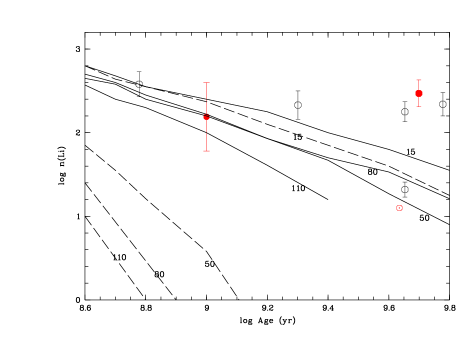
Figure 9: Same as Fig. 7, but a narrower age interval is shown. The empirical distribution is compared with the predictions of the models by Charbonnel & Talon (ct05 (2005)). The latter have been reconstructed starting from Fig. 2 in that paper. Different curves are for different initial rotational velocities (in km/s) as labeled. Solid curves correspond to model including waves + rotation, while dashed lines denote models including only waves.

5.4 Pop. I and Pop. II plateaus

In the previous sections we have definitively shown that stars with temperatures similar to the Sun are not necessarily heavily Li-depleted like the Sun is; instead, Li abundances of the majority of stars converge towards a plateau, whose value, on the order of $\log$ n(Li)$=2.3-2.5$, is close (although not identical) to that of Pop. II stars. However, the path/masses/timescales are different towards virtually this same average value of Li. The similarity of the plateau of Pop. I stars to the plateau of the significantly more metal-poor Pop. ii is indeed very intriguing and should be investigated on theoretical grounds. Figure 8 indeed suggests that there might be a sequence between old, solar-metallicity OCs and metal–poor less massive Pop. II stars, with Be 32 in the middle. This sequence is purely phenomenological and it does not provide insight into the depletion history of Pop. II stars or into whether they actually depleted some Li or not; nevertheless, it is tempting to interpret it as evidence that, whatever the initial Li abundance and whatever the mixing mechanism, the final Li abundance is the same for metal-poor Pop ii stars and more metal-rich ones. Those stars, like the Sun, that instead deplete a much larger amount of Li represent an exception.

6 Conclusions

We carried out a FLAMES/Giraffe survey of almost 160 candidate members of the old, metal-poor open cluster Be 32, with the goals of inferring membership and of studying the Li abundance pattern. To this aim, we derived radial velocities and Li abundances. Slightly more than half of the sample stars are confirmed as cluster members. This is a lower limit, since we may have missed some binaries due to the too short time coverage of our observations. The Li versus T_eff distribution of unevolved members overlaps with that of the slightly older, more metal-rich NGC 188, and with the upper envelope of M 67. At variance with the last, Be 32 does not show any dispersion in Li. The average abundance of stars with solar–like temperature is slightly below the Hyades but, within the margins of error, the same as for their counterparts in the intermediate age OCs, the upper envelope of M 67, and NGC 188. This confirms, on solid and statistically significant grounds, that, with exception of Li–poor stars like the Sun, Li abundances in solar-like Pop. I stars converge towards a plateau value, implying that Li cannot be used as an age indicator after about 0.5 Gyr. In addition, the plateau of old OCs is close to the plateau value of Pop. II stars. To our knowledge, none of the models including extra-mixing developed so far predicts the convergence toward a plateau at old ages.

Given their lower metallicity, Be 32 stars with temperature close to the Sun are less massive than the Sun. A comparison in a $\log$ n(Li)–mass diagram shows that these stars have depleted much less Li than the Hyades with similar mass. Our conclusion is that stars with different masses and metallicities, but very similar temperatures, converge at old ages to the same Li abundance, though following different Li depletion histories. This might also be true for halo stars.

[x]rccccccccccrc Sample stars.
ID RA DEC. Conf. B_DBT V(B–V)_DBT V(V–I)_DBT I_DBT V_lit. B–V_KM V–I_RS v_rad mf
J2000 (Km/s)
continued.
ID RA DEC. Conf. B_DBT V(B–V)_DBT V(V–I)_DBT I_DBT V_lit. B–V_KM V–I_RS v_rad mf
J2000 (Km/s)
74 6 58 05.410 6 25 40.18 B 16.840 15.846 15.855 14.798 15.862 0.956 1.042 105.4 $\pm 1.5$ m
77 6 57 56.856 6 24 26.47 B — — — — 15.889 0.871 0.910 — ?
84 6 58 09.005 6 28 55.83 A 16.567 15.953 15.948 15.196 15.955 0.598 0.742 $44.7\pm 2.4$ n
86 6 58 05.060 6 24 59.35 A 16.536 15.987 15.983 15.317 15.972 0.544 0.628 $111.5\pm 0.94$ n
91 6 58 00.353 6 27 44.37 A 16.745 15.969 15.970 15.082 16.001 0.744 0.883 $33.6\pm 0.14$ n
97 6 58 14.083 6 26 43.18 A 16.930 16.060 16.060 15.056 16.052 0.872 0.975 $104.8\pm 0.43$ m
99 6 58 00.174 6 26 39.60 B 16.862 16.073 16.073 15.161 16.069 0.781 0.895 $107.1\pm 1.2$ m
101 6 58 06.636 6 24 12.65 B 16.938 16.048 16.051 15.059 16.074 0.867 0.980 $34.1\pm 0.9$ n
106 6 58 04.028 6 24 08.09 A 16.807 16.108 16.108 15.303 16.099 0.717 0.786 $50.1\pm 0.43$ n
109 6 58 18.702 6 27 03.72 A 16.711 16.049 16.041 15.203 16.106 0.668 0.794 $104.2\pm 0.32$ m
110 6 57 54.792 6 28 22.07 B 16.698 16.042 16.032 15.183 16.112 0.649 0.828 $106.4\pm 2.2$ m
111 6 57 53.981 6 24 23.93 B 16.749 16.106 16.102 15.315 16.120 0.620 0.805 $106.3\pm 2$ m
117 6 58 13.277 6 26 02.88 B 16.943 16.133 16.136 15.225 16.156 0.766 0.879 $104.7\pm 1.2$ m
122 6 58 14.152 6 29 31.54 A 16.992 16.180 16.176 15.199 16.207 0.823 0.955 $105.3\pm 0.25$ m
127 6 58 08.191 6 24 35.48 A 16.868 16.247 16.243 15.483 16.249 0.603 0.755 $96.5\pm 1.25$ n
130 6 57 56.913 6 27 16.87 A 16.890 16.260 16.254 15.470 16.267 0.618 0.765 $105.0\pm 0.28$ m
137 6 58 15.058 6 26 40.60 B 17.335 16.286 16.291 15.136 16.333 1.019 1.108 $49.7\pm 1.4$ n
146 6 58 03.057 6 24 31.69 A 17.062 16.441 16.437 15.680 16.414 0.629 0.766 $105.2\pm 0.32$ m
147 6 58 17.988 6 29 43.94 A 16.961 16.401 16.388 15.612 16.426 0.586 0.744 $96.2\pm 0.59$ n
148 6 58 04.879 6 27 39.04 A 17.033 16.411 16.406 15.646 16.435 0.588 0.770 $71.1\pm 0.16$ n
154 6 58 16.781 6 26 11.06 B 17.058 16.459 16.452 15.695 16.481 0.583 0.722 $104.5\pm 2.4$ m
169 6 58 07.185 6 23 48.59 B 17.206 16.626 16.620 15.891 16.613 0.579 0.711 — ?
189 6 57 58.952 6 26 48.52 B 17.458 16.798 16.792 15.970 16.762 0.662 0.803 $105.2\pm 1.4$ m
193 6 58 02.247 6 29 21.35 A 17.362 16.768 16.759 15.981 16.785 0.605 0.780 $104.9\pm 0.84$ m
202 6 58 03.561 6 23 46.77 B 17.459 16.845 16.838 16.058 16.835 0.617 0.752 $107.1\pm 3.1$ m
206 6 58 14.715 6 27 02.31 B 17.431 16.814 16.808 16.044 16.844 0.604 0.701 $107.1\pm 2$ m
212 6 58 12.503 6 28 33.07 B 17.469 16.873 16.863 16.079 16.879 0.605 0.749 $63.3\pm 2.1$ n
213 6 58 16.427 6 23 34.95 B 17.450 16.848 16.841 16.072 16.881 0.605 0.760 $103.3\pm 1.9$ m
216 6 57 54.890 6 27 12.27 A 17.473 16.903 16.888 16.088 16.909 0.570 0.741 $104.8\pm 1.3$ m
218 6 58 04.891 6 23 31.10 B 17.543 16.944 16.936 16.169 16.929 0.627 0.713 $108.6\pm 3.6$ n
219 6 58 15.312 6 28 15.59 A 17.520 16.886 16.877 16.067 16.929 0.632 0.760 $110.8\pm 0.8$ n
220 6 58 10.153 6 23 51.84 B 17.561 16.918 16.913 16.120 16.930 0.633 0.791 $81.3\pm 3.0$ n
222 6 58 16.404 6 27 15.53 B 17.509 16.903 16.895 16.125 16.960 0.571 0.738 $105.3\pm 2.4$ m
231 6 58 14.010 6 26 57.99 A,B 17.589 16.983 16.977 16.222 17.019 0.589 0.695 $104.8\pm 1.0$ m
236 6 58 02.398 6 26 57.18 A — — — — 17.065 0.704 0.833 $105.5\pm 0.57$ m
240 6 58 12.220 6 25 57.42 A,B 17.797 17.073 17.078 16.292 17.124 0.658 0.804 $35.6\pm 1.1$ n
241 6 57 57.665 6 25 41.09 A,B 17.773 17.152 17.146 16.371 17.135 0.591 0.759 $105.8\pm 0.54$ m
245 6 58 02.865 6 25 09.94 A,B — — — — 17.167 0.616 0.737 $110.6\pm 0.4$ n
254 6 58 01.182 6 29 00.09 A 17.925 17.257 17.249 16.403 17.279 0.674 0.835 $45.7\pm 1.0$ n
265 6 58 12.307 6 24 50.80 A,B 18.004 17.334 17.336 16.586 17.342 0.679 0.737 $104.7\pm 1.2$ m
271 6 58 16.474 6 24 00.78 A,B 17.955 17.317 17.312 16.529 17.355 0.641 0.770 $105.2\pm 1.11$ m
276 6 57 58.540 6 28 06.48 A,B 18.020 17.376 17.368 16.543 17.396 0.649 0.823 $104.8\pm 0.32$ m
277 6 57 53.234 6 27 03.85 A,B 18.046 17.440 17.427 16.609 17.398 0.513 0.831 $104.8\pm 0.7$ m
278 6 58 06.158 6 26 01.56 A,B 18.075 17.419 17.418 16.652 17.410 0.643 0.734 $104.7\pm 1.92$ m
288 6 58 08.217 6 26 28.77 A,B 18.137 17.414 17.417 16.619 17.447 0.636 0.806 $107.6\pm 0.6$ m
289 6 58 05.985 6 25 23.23 A,B 18.154 17.447 17.445 16.615 17.454 0.670 0.807 $105.6\pm 0.9$ m
292 6 58 06.568 6 26 53.29 A,B 18.103 17.470 17.465 16.691 17.485 0.579 0.752 $92.5\pm 1.0$ n
294 6 58 15.206 6 29 36.09 A,B 18.115 17.464 17.458 16.644 17.491 0.677 0.814 $63.6\pm 1.0$ n
299 6 58 01.374 6 27 16.75 A,B 18.206 17.524 17.521 16.712 17.512 0.645 0.777 $105.3\pm 1.3$ m
311 6 58 05.745 6 23 45.05 A 18.263 17.577 17.569 16.697 17.573 0.686 0.828 $104.1\pm 0.5$ m
313 6 58 06.532 6 25 38.80 A,B 18.282 17.571 17.580 16.845 17.597 0.635 0.751 $105.1\pm 1.1$ m
314 6 58 10.331 6 27 12.53 A,B 18.208 17.575 17.566 16.754 17.602 0.616 0.794 $107.6\pm 0.6$ m
315 6 58 00.111 6 27 07.30 A 18.287 17.601 17.596 16.757 17.607 0.600 0.822 $105.7\pm 1.3$ m
316 6 58 10.618 6 24 23.52 A,B 18.276 17.608 17.606 16.810 17.610 0.670 0.761 $105.8\pm 0.5$ m
317 6 58 16.862 6 26 32.37 A,B 18.301 17.591 17.584 16.691 17.612 0.694 0.850 $110.0\pm 1.6$ n
325 6 57 55.799 6 28 12.39 A,B 18.257 17.584 17.575 16.717 17.635 0.671 0.840 $105.3\pm 0.6$ m
326 6 58 17.239 6 23 49.38 A,B 18.222 17.610 17.601 16.812 17.645 0.625 0.771 $114.1\pm 1.13$ n
331 6 58 06.080 6 26 36.12 A,B 18.392 17.684 17.688 16.911 17.679 0.692 0.784 $46.7\pm 2$ n
333 6 58 14.218 6 25 31.96 A — — — — 17.707 0.680 0.765 $104.8\pm 0.7$ m
344 6 57 58.305 6 25 58.35 A 18.503 17.792 17.790 16.946 17.768 0.707 0.873 $100.1\pm 1.0$ n
352 6 58 18.582 6 29 32.81 A,B 18.436 17.768 17.760 16.913 17.808 0.678 0.819 $104.5\pm 1$ m
357 6 58 00.620 6 24 29.96 A,B 18.569 17.878 17.879 17.094 17.839 0.677 0.773 $104.5\pm 1.5$ m
362 6 58 10.854 6 26 43.75 A,B — — — — 17.878 0.625 0.797 $51.7\pm 5$ n
364 6 58 04.497 6 26 55.95 A,B 18.666 17.897 17.909 17.138 17.880 0.723 0.803 $105.4\pm 1.2$ m
367 6 58 09.763 6 23 37.42 A,B 18.523 17.889 17.876 17.029 17.896 0.658 0.820 $40.5\pm 0.3$ n
369 6 57 54.006 6 24 58.68 A,B 18.650 17.955 17.955 17.149 17.910 0.755 0.879 $103.4\pm 1.0$ m
371 6 57 58.413 6 23 49.71 A,B 18.652 17.941 17.939 17.103 17.934 0.723 0.877 $106.0\pm 0.8$ m
373 6 57 59.759 6 23 29.26 A,B 18.602 17.937 17.935 17.149 17.952 0.609 0.777 $70.2\pm 1.5$ n
374 6 58 10.035 6 26 56.43 A 18.670 17.947 17.947 17.118 17.965 0.669 0.775 $105.2\pm 0.7$ m
927 6 58 05.163 6 23 01.21 A 14.268 12.889 12.904 11.461 12.896 — 1.425 $105.5\pm 0.3$ m
1043 6 58 11.169 6 22 14.52 B 16.785 15.841 15.845 14.794 15.848 — 1.074 $37.2\pm 1.6$ n
1047 6 57 51.082 6 20 53.46 B — — — — 15.912 — 0.929 $104.9\pm 2.3$ m
1049 6 58 03.201 6 21 12.02 B — — — — 15.917 — 0.749 $43.5\pm 6.3$ n
1050 6 58 03.329 6 22 25.01 B 16.887 15.894 15.899 14.805 15.923 — 1.115 $105.3\pm 1.2$ m
1051 6 58 28.829 6 20 59.65 B — — — — 15.964 — 0.983 — ?
1057 6 58 20.765 6 22 07.75 B 16.761 16.007 16.006 15.131 15.991 — 0.896 $42.0\pm 2.1$ n
1059 6 57 44.117 6 24 57.58 B — — — — 16.006 — 0.623 $106.8\pm 3.8$ m
1066 6 58 24.787 6 24 09.94 B 16.756 16.082 16.077 15.260 16.077 — 0.801 $105.5\pm 1.2$ m
1069 6 57 52.859 6 29 07.52 A — — — — 16.082 — 0.668 $99.5\pm 1.6$ n
1070 6 58 04.031 6 22 57.96 A 16.728 16.066 16.060 15.243 16.083 — 0.818 $104.8\pm 0.3$ m
1072 6 58 23.376 6 27 00.93 A 17.113 16.090 16.091 14.924 16.089 — 1.153 $51.8\pm 0.2$ n
1073 6 57 43.108 6 22 07.05 B — — — — 16.095 — 0.708 $69.7\pm 5.6$ n
1074 6 58 19.457 6 22 01.50 B 16.640 16.128 16.123 15.480 16.103 — 0.667 $58.9\pm 1.4$ n
1075 6 58 21.900 6 22 13.24 A 16.662 16.126 16.119 15.425 16.108 — 0.711 $27.0\pm 1.1$ n
1077 6 58 26.626 6 30 12.54 B — — — — 16.123 — 0.720 $106.5\pm 1.8$ m
1078 6 57 51.039 6 29 04.62 B — — — — 16.127 — 0.782 $14.6\pm 5.2$ n
1082 6 58 27.554 6 24 16.90 B — — — — 16.163 — 0.801 — ?
1084 6 58 10.628 6 20 40.14 B — — — — 16.177 — 0.810 $104.4\pm 1.7$ m
1088 6 57 52.147 6 29 18.22 B — — — — 16.204 — 0.850 $105.8\pm 2.0$ m
1090 6 58 14.337 6 22 57.76 A 16.726 16.223 16.217 15.573 16.216 — 0.638 $106.5\pm 4.5$ m, SB2?
1092 6 58 23.454 6 28 52.21 A 16.844 16.231 16.225 15.462 16.220 — 0.744 $105.2\pm 0.6$ m
1097 6 58 10.641 6 30 41.64 A 16.819 16.250 16.233 15.414 16.258 — 0.789 $104.6\pm 0.2$ m
1101 6 57 54.904 6 22 58.15 B 16.858 16.238 16.232 15.462 16.275 — 0.780 $105.5\pm 1.3$ m
1102 6 58 15.248 6 21 37.54 B 16.962 16.363 16.346 15.495 16.289 — 0.813 $84.7\pm 2.9$ n
1105 6 58 03.716 6 20 16.81 B — — — — 16.300 — 0.784 $103.9\pm 1.7$ m
1112 6 58 20.650 6 31 00.58 B — — — — 16.330 — 0.913 $39.9\pm 0.5$ n
1113 6 58 20.285 6 23 48.40 A 16.947 16.335 16.329 15.565 16.333 — 0.775 $104.9\pm 0.7$ m
1114 6 57 51.759 6 27 17.88 A 16.922 16.342 16.329 15.541 16.336 — 0.769 $101.7\pm 0.9$ n
1116 6 57 45.696 6 24 02.85 B — — — — 16.354 — 0.738 $75.0\pm 5.9$ n
1117 6 57 51.055 6 31 13.59 A — — — — 16.376 — 1.065 $105.0\pm 0.2$ m
1121 6 58 03.681 6 22 17.30 A 17.255 16.362 16.361 15.319 16.386 — 1.067 $104.8\pm 0.4$ m
1122 6 58 24.188 6 21 04.34 B — — — — 16.393 — 1.122 $43.4\pm 1.6$ n
1123 6 58 21.389 6 30 32.08 A — — — — 16.420 — 0.741 $54.1\pm 0.4$ n
1126 6 57 59.971 6 30 05.96 A 17.171 16.353 16.352 15.395 16.431 — 0.966 $17.9\pm 0.5$ n
1128 6 58 30.891 6 23 30.75 B — — — — 16.434 — 0.738 $105.0\pm 1.0$ m
1129 6 57 50.796 6 27 03.39 B 17.300 16.481 16.476 15.482 16.435 — 0.946 $58.7\pm 2.7$ n
1130 6 58 14.736 6 31 19.87 A — — — — 16.450 — 0.740 $107.3\pm 0.4$ m
1141 6 58 20.329 6 30 36.64 A — — — — 16.531 — 0.693 $105.2\pm 0.5$ m
1144 6 57 50.902 6 21 57.44 A — — — — 16.555 — 0.776 $59.5\pm 0.3$ n
1150 6 58 10.245 6 21 06.25 A — — — — 16.590 — 0.774 $106.1\pm 0.8$ m
1153 6 58 09.489 6 21 07.21 B — — — — 16.629 — 0.787 $104.5\pm 2.9$ m
1156 6 57 51.474 6 22 38.53 B — — — — 16.646 — 0.775 $106.0\pm 2.2$ m
1161 6 57 48.933 6 22 14.65 B — — — — 16.695 — 0.751 $62.2\pm 3.0$ n
1164 6 58 25.577 6 29 39.85 A — — — — 16.707 — 0.711 $95.9\pm 0.2$ n
1179 6 58 17.498 6 20 46.12 B — — — — 16.799 — 0.759 $35.4\pm 4.4$ n
1181 6 57 54.593 6 21 30.34 A — — — — 16.809 — 0.808 $-15.8\pm 1.0$ n
1187 6 58 21.059 6 24 31.50 A 17.561 16.853 16.851 16.015 16.829 — 0.814 $34.9\pm 0.3$ n
1195 6 58 20.695 6 19 17.52 B — — — — 16.880 — 0.798 $104.4\pm 1.7$ m
1212 6 58 06.229 6 29 45.40 A 17.587 16.972 16.960 16.140 16.955 — 0.806 $104.2\pm 0.9$ m
1228 6 57 51.634 6 27 48.18 A,B 17.675 17.070 17.056 16.224 17.028 — 0.776 $105.1\pm 0.8$ m
1231 6 57 57.805 6 30 26.93 A,B 17.636 17.039 17.027 16.227 17.060 — 0.693 $105.8\pm 1.4$ m
1238 6 57 53.881 6 22 43.21 A,B — — — — 17.077 — 0.734 $98.2\pm 1.5$ n
1241 6 57 52.746 6 26 48.95 A,B 17.607 17.109 17.083 16.260 17.087 — 0.816 $105.4\pm 0.6$ m
1245 6 58 08.660 6 21 11.52 A,B — — — — 17.116 — 0.762 $40.3\pm 0.9$ n
1250 6 57 46.565 6 23 34.51 A,B — — — — 17.143 — 0.789 $64.7\pm 0.8$ n
1257 6 58 06.810 6 21 30.85 A,B — — — — 17.172 — 0.785 $105.1\pm 0.3$ m
1263 6 58 11.569 6 31 06.92 A,B — — — — 17.183 — 0.794 $104.4\pm 1.5$ m
1265 6 58 25.849 6 20 00.02 A,B — — — — 17.214 — 0.763 $48.9\pm 1.2$ n
1279 6 58 19.836 6 24 48.43 A,B 17.926 17.285 17.282 16.517 17.268 — 0.770 $105.6\pm 0.4$ m
1300 6 58 24.200 6 26 52.86 A 18.032 17.399 17.385 16.530 17.338 — 0.817 $103.0\pm 1.2$ m
1302 6 58 23.298 6 24 22.61 A,B 17.976 17.374 17.366 16.588 17.350 — 0.791 $79.6\pm 0.3$ n
1327 6 58 19.564 6 26 46.99 A,B 18.110 17.454 17.447 16.629 17.419 — 0.749 $104.9\pm 0.2$ m
1337 6 58 20.259 6 22 51.31 A 18.130 17.500 17.490 16.666 17.474 — 0.824 $105.1\pm 1.0$ m
1340 6 57 58.583 6 23 05.37 A,B 18.143 17.473 17.463 16.599 17.487 — 0.859 $110.6\pm 0.2$ n
1344 6 58 20.635 6 29 20.49 A,B 18.210 17.538 17.527 16.652 17.496 — 0.830 $54.8\pm 0.5$ n
1347 6 58 25.123 6 24 50.62 A,B 18.113 17.559 17.545 16.769 17.514 — 0.738 $-8.4\pm 0.7$ n
1349 6 58 06.074 6 20 55.42 A,B — — — — 17.521 — 0.834 $105.2\pm 1.3$ m
1350 6 58 07.071 6 29 51.00 A — — — — 17.534 — 0.735 $-7.1\pm 0.8$ n
1358 6 58 22.953 6 26 07.86 A,B 18.232 17.585 17.575 16.735 17.564 — 0.790 $55.5\pm 1.4$ n
1359 6 58 16.363 6 20 30.20 A,B — — — — 17.565 — 0.838 $112.2\pm 0.7$ n
1366 6 57 47.025 6 21 04.33 A,B — — — — 17.599 — 0.783 $6.9\pm 2.5$ n
1369 6 58 00.536 6 29 46.04 A,B 18.178 17.578 17.564 16.741 17.610 — 0.834 $96.8\pm 2.3$ n
1376 6 57 56.129 6 22 25.39 A,B 18.209 17.636 17.621 16.815 17.645 — 0.786 $55.2\pm 0.8$ n
1384 6 58 20.728 6 20 07.11 A,B — — — — 17.671 — 0.871 $105.2\pm 0.7$ m
1396 6 57 57.167 6 22 05.87 A,B — — — — 17.729 — 0.837 $84.2\pm 0.7$ n
1398 6 57 51.821 6 23 45.15 A,B — — — — 17.739 — 0.800 $2.2\pm 3.0$ n
1404 6 58 16.159 6 22 39.07 A,B 18.456 17.753 17.753 16.945 17.753 — 0.833 $105.2\pm 1.3$ m
1405 6 57 58.352 6 22 07.42 A,B 18.387 17.735 17.724 16.864 17.757 — 0.855 $104.6\pm 0.84$ m
1407 6 58 00.780 6 31 46.58 A,B — — — — 17.776 — 0.891 $77.5\pm 0.3$ n
1410 6 57 54.497 6 20 49.36 A,B — — — — 17.788 — 0.857 $53.8\pm 3.7$ n
1421 6 58 21.122 6 31 28.66 A,B — — — — 17.820 — 0.864 $41.3\pm 2.4$ n
1429 6 58 23.617 6 31 19.37 A,B — — — — 17.864 — 0.833 $106.3\pm 1.3$ m
1433 6 57 47.116 6 24 27.06 A,B — — — — 17.890 — 0.906 $61.3\pm 0.9$ n
1438 6 58 06.609 6 21 07.58 A — — — — 17.913 — 0.874 $105.9\pm 1.3$ m
1448 6 58 18.537 6 21 09.20 A,B — — — — 17.943 — 0.812 $56.4\pm 1.4$ n
1453 6 58 09.106 6 30 41.55 A,B 18.671 17.977 17.959 16.986 17.955 — 0.873 $104.3\pm 0.6$ m
1457 6 58 15.196 6 30 33.37 A,B 18.691 17.966 17.947 16.939 17.962 — 0.890 $73.3\pm 0.5$ n

[x]rcccc Final results of our analysis.
ID (B–V)₀ T_eff EW(Li) $\log$ n(Li)
(K) (mÅ)

continued.
ID (B–V)₀ T_eff EW(Li) $\log$ n(Li)
(K) (mÅ)

97 0.730 5233 $40\pm 10$ $1.53\pm 0.15$
109 0.522 6024 $\leq 16$ $\leq 1.88$
117 0.670 5401 $42\pm 6$ $1.76\pm 0.14$
122 0.672 5395 $\leq 25$ $\leq 1.59$
130 0.490 6152 $66\pm 7$ $2.73\pm 0.12$
146 0.481 6189 $55\pm 5$ $2.66\pm 0.11$
154 0.459 6282 $58\pm 12$ $2.77\pm 0.15$
193 0.454 6303 $38\pm 7$ $2.57\pm 0.15$
206 0.477 6206 $60\pm 7$ $2.72\pm 0.11$
216 0.430 6408 $63\pm 2$ $2.92\pm 0.13$
231 0.466 6252 $47\pm 2$ $2.63\pm 0.13$
236 0.560^a 5878 $48\pm 3$ $2.31\pm 0.15$
241 0.481 6189 $57\pm 4$ $2.68\pm 0.14$
265 0.530 5992 $76\pm 6$ $2.67\pm 0.10$
271 0.498 6119 $59\pm 7$ $2.64\pm 0.12$
276 0.504 6095 $51\pm 9$ $2.54\pm 0.13$
277 0.466 6252 $47\pm 6$ $2.63\pm 0.10$
278 0.516 6047 $57\pm 6$ $2.56\pm 0.12$
288 0.583 5793 $53\pm 4$ $2.28\pm 0.10$
289 0.567 5852 $43\pm 6$ $2.23\pm 0.12$
299 0.542 5946 $65\pm 6$ $2.54\pm 0.11$
311 0.546 5931 $58\pm 6$ $2.46\pm 0.12$
313 0.500 6111 $60\pm 9$ $2.64\pm 0.13$
314 0.493 6140 $59\pm 1$ $2.66\pm 0.16$
315 0.546 5931 $74\pm 7$ $2.60\pm 0.11$
316 0.528 6000 $83\pm 13$ $2.73\pm 0.14$
325 0.533 5981 $63\pm 8$ $2.55\pm 0.13$
333 0.540 ^a 5954 $60\pm 10$ $2.50\pm 0.14$
352 0.528 6000 $70\pm 11$ $2.63\pm 0.14$
357 0.551 5912 $46\pm 7$ $2.32\pm 0.17$
364 0.580^a,∗ 5804 $49\pm 7$ $2.25\pm 0.14$
369 0.555 5897 $93\pm 4$ $2.71\pm 0.15$
371 0.571 5837 $84\pm 12$ $2.59\pm 0.14$
374 0.583 5793 $50\pm 10$ $2.25\pm 0.15$
1050 0.853 4920 $65\pm 5$ $1.45\pm 0.16$
1070 0.522 6024 $25\pm 7$ $2.12\pm 0.25$
1092 0.473 6222 $33\pm 5$ $2.44\pm 0.15$
1113 0.472 6227 $38\pm 3$ $2.51\pm 0.15$
1121 0.753 5233 $\leq 17$ $\leq 1.82$
1128 0.450^b 6320 $31\pm 6$ $2.49\pm 0.14$
1130 0.450^b 6320 $\leq 20$ $\leq 2.27$
1150 0.480^b 6193 $55\pm 5$ $2.56\pm 0.12$
1212 0.475 6214 $55\pm 7$ $2.68\pm 0.12$
1228 0.465 6256 $63\pm 4$ $2.79\pm 0.12$
1231 0.457 6290 $56\pm 6$ $2.76\pm 0.11$
1241 0.530^b,∗ 5992 $52\pm 5$ $2.46\pm 0.11$
1257 0.490^b 6152 $53\pm 9$ $2.61\pm 0.12$
1263 0.490^b 6152 $60\pm 7$ $2.68\pm 0.12$
1279 0.501 6107 $61\pm 10$ $2.65\pm 0.13$
1300 0.493 6140 $42\pm 6$ $2.48\pm 0.12$
1327 0.516 6047 $37\pm 10$ $2.34\pm 0.19$
1337 0.490 6152 $44\pm 5$ $2.51\pm 0.12$
1349 0.530 ^b 5992 $85\pm 9$ $2.74\pm 0.12$
1384 0.570 ^b 5841 $59\pm 6$ $2.39\pm 0.12$
1405 0.512 6063 $65\pm 10$ $2.64\pm 0.14$
1438 0.570 ^b 5841 $70\pm 12$ $2.48\pm 0.15$
1453 0.554 5900 $49\pm 9$ $2.34\pm 0.15$

$a$: B–V from Richtler & Sagar (rs00 (2000))
$b$: (B–V)₀ derived from (V–I) (see text)
$*$: B–V from D’Orazi et al. available, but not used (see text)