A 3D radiative transfer framework: IV. spherical & cylindrical coordinate systems

Abstract

Aims. We extend our framework for 3D radiative transfer calculations with a non-local operator splitting methods along (full) characteristics to spherical and cylindrical coordinate systems. These coordinate systems are better suited to a number of physical problems than Cartesian coordinates.

Methods. The scattering problem for line transfer is solved via means of an operator splitting (OS) technique. The formal solution is based on a full characteristics method. The approximate $\Lambda$ operator is constructed considering nearest neighbors exactly. The code is parallelized over both wavelength and solid angle using the MPI library.

Results. We present the results of several test cases with different values of the thermalization parameter for the different coordinate systems. The results are directly compared to 1D plane parallel tests. The 3D results agree very well with the well-tested 1D calculations.

Conclusions. Advances in modern computers will make realistic 3D radiative transfer calculations possible in the near future.

1 Introduction

In Hauschildt & Baron (2006, hereafter: Paper I), Baron & Hauschildt (2007, hereafter: Paper II) and (Hauschildt & Baron 2008, hereafter: Paper III) we described a framework for the solution of the radiative transfer equation for scattering continua and lines in 3D (when we say 3D we mean three spatial dimensions, plus three momentum dimensions) for the time independent, static case using full characteristics based on voxels in Cartesian coordinates. Cartesian coordinates are by no means an optimal choice for many 3D physical systems, for example supernova atmospheres are better described in 3D spherical and accretion disks are better described in 3D cylindrical coordinates. These coordinate systems make it a little harder and computationally more expensive to track the characteristics through the curvilinear voxel grid, however, this is more than overcompensated by the higher efficiency of voxel usage, for example consider putting a roughly spherical structure where density and composition vary strongly with radius into a Cartesian coordinate system cube.

We describe our method, its rate of convergence, and present comparisons to our well-tested 1-D calculations.

2 Method

In the following discussion we use notation of Papers I – III. The basic framework and the methods used for the formal solution and the solution of the scattering problem via operator splitting are discussed in detail in Papers I and II and will not be repeated here.

We use a “full characteristics” approach that completely tracks a set of characteristics of the radiative transfer equation from the inner or outer boundary through the computational domain to their exit voxels and takes care that each voxel is hit by at least one characteristic per solid angle. One characteristic is started at each boundary voxel and then tracked through the voxel grid until it leaves the other boundary. The direction of a bundle of characteristics is determined by a set of solid angles $(\theta,\varphi)$ which correspond to a normalized momentum space vector $(p_{x},p_{y},p_{z})$.

In contrast to the case of Cartesian coordinates the volumes of the voxels can be vastly different in spherical and Cartesian coordinate systems. Therefore, tracking a characteristic across the voxel grid is done using an adaptive stepsize control along the characteristic so that a characteristic steps from one voxel to its neighbor in the direction of the characteristic. In addition, we make sure that each voxel is hit by at least one characteristic for each solid angle, which is important for the inner (small radii) voxels.

The code is parallelized as described in Papers I and II.

3 spherical coordinates

3.1 Testing environment

We use the framework discussed in Paper I and II as the baseline for the line transfer problems discussed in this paper. Our basic setup is similar to that discussed in Paper II. We use a sphere with a grey continuum opacity parameterized by a power law in the continuum optical depth ${\tau_{\rm std}}$. The basic model parameters are

1. Inner radius $r_{c}=10^{10}\,$cm, outer radius $\hbox{$r_{\rm out}$}=2\times 10^{10}\,$cm (large test case) or $\hbox{$r_{\rm out}$}=1.1\times 10^{10}\,$cm (small test case).

2. Minimum optical depth in the continuum $\tau_{\rm std}^{\rm min}=10^{-4}$ and maximum optical depth in the continuum $\tau_{\rm std}^{\rm max}=10^{8}$.

3. Constant temperature with $\hbox{$\,T_{\rm eff}$}=10^{4}$ K, therefore, the Planck function $B$ is also constant.

4. Outer boundary condition $I_{\rm bc}^{-}\equiv 0$ and diffusion inner boundary condition for all wavelengths.

5. Continuum extinction $\chi_{c}=C/r^{6}$, with the constant $C$ fixed by the radius and optical depth grids, for the continuum tests, $\chi_{c}=C$ for the line transfer tests

6. Parameterized coherent & isotropic continuum scattering by defining

   $$\chi_{c}=\epsilon_{c}\kappa_{c}+(1-\epsilon_{c})\sigma_{c}$$

   with $0\leq\epsilon_{c}\leq 1$. $\kappa_{c}$ and $\sigma_{c}$ are the continuum absorption and scattering coefficients.

This problem is used because the results can be directly compared with the results obtained with a 1D spherical radiation transport code Hauschildt (1992) to assess the accuracy of the method. The sphere is put at the center of the 3D grid. The radial grid in the 3D coordinates is logarithmic in ${\tau_{\rm std}}$ and has, therefore, highly variable spacing in $r$. In 3D spherical coordinates $(r,\theta_{c},\phi_{c})$ (note: the subscript $c$ indicates a coordinate in order to distinguish with the solid angle $\Omega=(\theta,\phi)$) we use regular grid in $(\theta_{c},\phi_{c})$ with resolutions given below. In the tests with cylindrical coordinates $(\rho,\phi_{c},z)$ we use a regular grid in $z$ and $\phi_{c}$ and a variable grid in $\rho$. The solid angle space was discretized in $(\theta,\phi)$ with $n_{\theta}=n_{\phi}$ if not stated otherwise. In the following we discuss the results of various tests. In all tests we use the full characteristics method for the 3D RT solution.

The line of the simple 2-level model atom is parameterized by the ratio of the profile averaged line opacity $\chi_{l}$ to the continuum opacity $\chi_{c}$ and the line thermalization parameter $\epsilon_{l}$. For the test cases presented below, we have used $\chi_{c}={\rm const}$, $\epsilon_{c}=1$, and a grey temperature structure. We set $\chi_{l}/\chi_{c}=10^{6}$ to simulate a strong line, with varying $\epsilon_{l}$ (see below). With this setup, the optical depths as seen in the line range from $10^{-2}$ to $10^{6}$. We use 32 wavelength points to model the full line profile, including wavelengths outside the line for the continuum. We did not require the line to thermalize at the center of the test configurations, this is a typical situation for a full 3D configuration as the location (or even existence) of the thermalization depths becomes more ambiguous than in the 1D case.

In the following we discuss the results of various tests. Unless otherwise stated, the tests were run on parallel computers using 4 to 512 CPUs (depending on the test). In spherical coordinates we use a voxel grid with $(n_{r},n_{\theta_{c}},n_{\phi_{c}})=(65,33,65)$ voxels, this corresponds to an angular resolution of about 5.5 degrees in $\theta_{c}$ and $\phi_{c}$. Projected on the surface of the Earth, this means that Europe is covered by about 43 voxels. The spherical test cases use incoming intensities of zero at the outside ($R_{\rm max})$ and $I=B$ at the inside (($R_{\rm min})$.

3.2 Results

3.2.1 Continuum tests

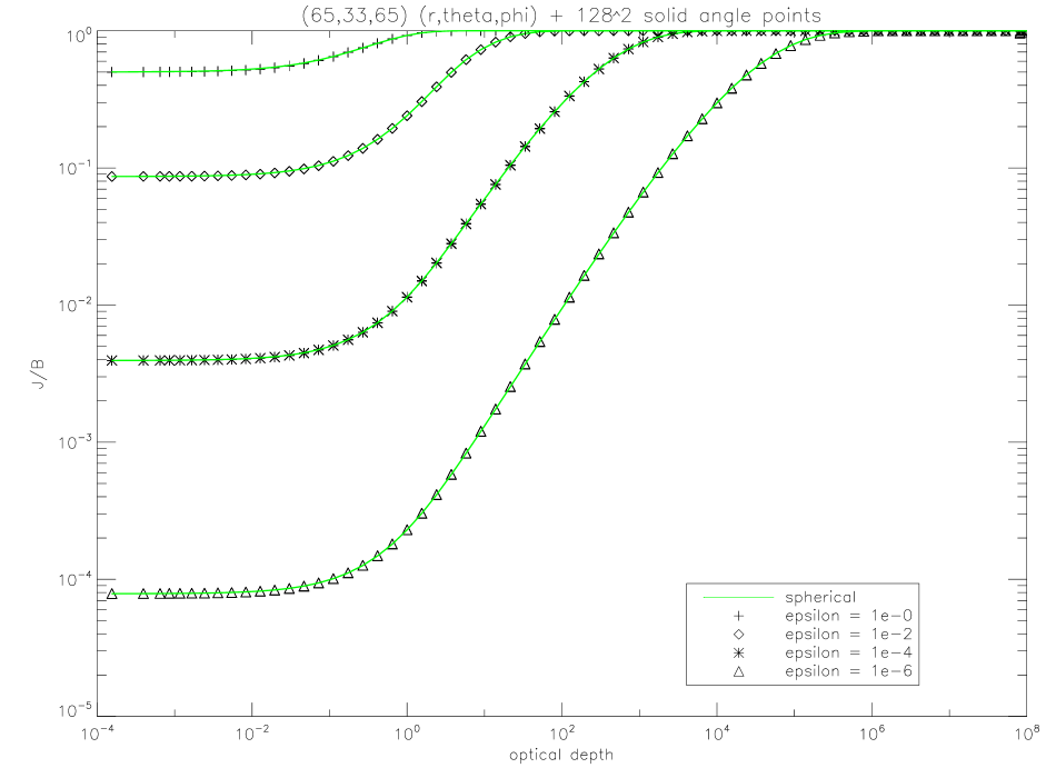
Figure 1: The ratio of the mean intensity $J$ and the Planck function $B$ as function of the radial optical depth ${\tau_{\rm std}}$ for the ’large’ test case in spherical coordinates and different values $\epsilon_{c}$. The optical depth is measured along the radius $r$.

In Fig. 1 we show the results for 3D continuum transfer with 3D spherical coordinates for various values of the thermalization parameter $\epsilon_{c}$. The results are compared to 1D results (full line). In all cases, the agreement is excellent, even for the case with $\epsilon_{c}=10^{-6}$. Compared to paper I the agreement is better, this is caused by the better discretization of a spherical configuration in spherical coordinates, rather than fitting a sphere into a Cartesian grid. It illustrates the importance of adapted coordinate systems to obtain the optimal mix between computational efficiency and numerical accuracy.

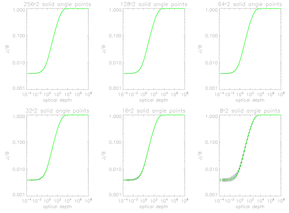
Figure 2: Effect of solid angle resolution on the results of the 3D calculations. The plots show the results for the ’small’ continuum test case in spherical coordinates with $\epsilon_{c}=10^{-4}$ and for various solid angle resolutions with $\nu_{\theta}=n_{\varphi}$ from $(256,256)$ to $(8,8)$. Full line: results of the 1D calculation, dots: results from the 3D calculations.

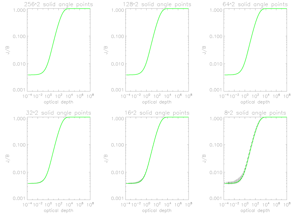
Figure 3: Effect of solid angle resolution on the results of the 3D calculations in spherical coordinates. The plots show the results for the ’large’ continuum test case with $\epsilon_{c}=10^{-4}$ and for various solid angle resolutions with $\nu_{\theta}=n_{\varphi}$ from $(256,256)$ to $(8,8)$. Full line: results of the 1D calculation, dots: results from the 3D calculations.

Good coverage of the solid angle is important for 3D transfer. The 1D code automatically adjusts the angle coverage related to the geometry of the configuration, however, in the 3D code the solid angles have to be prescribed. In Fig. 2 we demonstrate the importance of solid angle sampling for a ’small’ test case with $\epsilon_{c}=10^{-4}$. The plots show the ratio $J/B$ as function of radial optical depth for various solid angle samplings and for all $(\phi_{c},\theta_{c})$ compared to the 1D results. It is immediately clear that for the ’small’ test case a solid angle sampling of $64^{2}$ points or more is reasonable, but that $16^{2}$ or less points result in a considerable scatter of the results. This result does not depend strongly on the radial extension of the configuration, as shown in Fig. 3.

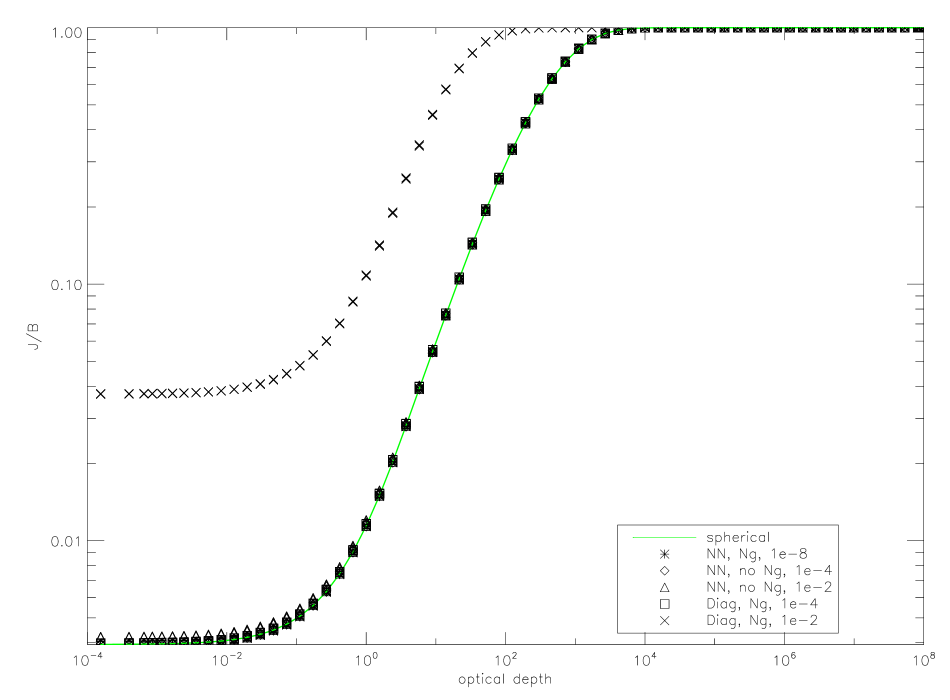
Figure 5: Effects of relaxing the convergence criterions on the results of the 3D calculations in spherical coordinates. The plots show the results for the ’large’ continuum test case with $\epsilon_{c}=10^{-4}$ and for various convergence limits for nearest neighbor (NN) and diagonal (Diag) ${\Lambda^{*}}$ operators with and without Ng acceleration. The numbers are the maximum allowed relative change over all voxels used to halt the iterations. Full line: results of the 1D calculation, dots: results from the 3D calculations.

The convergence rate of the nearest neighbor ${\Lambda^{*}}$ ($3^{3}$ neighbor voxels are considered in the ${\Lambda^{*}}$, see Paper I for details) with Ng acceleration is virtually identical to that of the 1D tri-diagonal ${\Lambda^{*}}$ case, cf. Fig. 4. The importance of a non-local ${\Lambda^{*}}$ for good convergence in the 3D case can be seen by comparing the results obtained with a local (diagonal) ${\Lambda^{*}}$. Its convergence with Ng acceleration is actually worse than that of the non-local ${\Lambda^{*}}$ without Ng acceleration. The excellent convergence of the non-local ${\Lambda^{*}}$ can be used to reduce the computing time by using a less stringent convergence criterion that still gives results accurate enough for a particular application. One has to be careful to be not too aggressive in relaxing the convergence criterion. This is highlighted in Fig. 5 where the results for the large test case are shown for different combinations of ${\Lambda^{*}}$ with Ng acceleration and difference convergence limits. It is obvious that the combination of Ng acceleration and a relatively large convergence limit with a local (diagonal) ${\Lambda^{*}}$ is not acceptable, whereas the same convergence limit ($10^{-2}$ maximum relative change of $J$) with a non-local (nearest neighbor) ${\Lambda^{*}}$ gives usable results even without Ng acceleration. Setting a convergence limit of $10^{-4}$ gives reasonable results in all test cases and can reduce computing time by about 50%.

With 128 MPI processes on the SGI ICE system of the Höchstleistungs Rechenzentrum Nord (HLRN) the continuum test with $\epsilon=10^{-4}$ and $n_{r}=n_{\phi}=65$ and $n_{\theta}=33$ spatial points and $256^{2}$ solid angle points requires 16 iterations and 1543 s wallclock time, where a formal solution takes about 80 s, the construction of the non-local ${\Lambda^{*}}$ about 140 s and about 1.6 s are used for the solution of the operator splitting step. For the same case with $64^{2}$ solid angles the total wallclock time is 230 s. The memory requirements are about 45MB/process.

3.2.2 Line tests

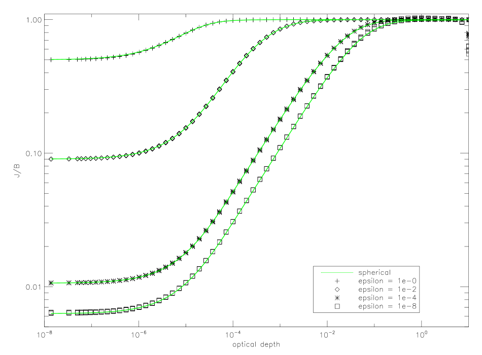
Figure 6: The ratio of the line mean intensity ${\bar{J}}$ and the Planck function $B$ as function of the radial optical depth ${\tau_{\rm std}}$ for the ’large’ test case in spherical coordinates for different values of $\epsilon_{l}$. The optical depth is measured along the radius $r$.

In Fig. 6 we show the results of a comparison of the ratio of the line mean intensities ${\bar{J}}$ and the Planck function $B$ for the ’large’ test case and various values of $\epsilon_{l}$. The 1D comparison models assume a diffusive inner boundary condition, whereas the 3D models use $I=B$ as the boundary condition for the inner boundary. Therefore, the models will differ close to the inner boundary. Away from the inner boundary the results of the 1D and 3D calculations agree very well with each other. The number of iterations required to reach a prescribed accuracy is similar to the continuum tests described above. This shows that the quality of the 3D calculations match the 1D results, which is very important for future applications.

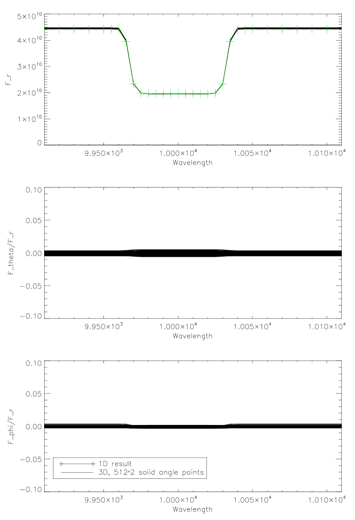
Figure 8: Flux vectors in the outermost voxels for the line transfer test in spherical coordinates with $\epsilon_{l}=1$ and $512^{2}$ solid angle points. The top panel shows the radial component $F_{r}$ of the voxel flux vector compared to the results for the 1D comparison calculation. The middle and bottom panels show the ratio of the polar $F_{\theta}$ and azimuthal $F_{\phi}$ flux components to $F_{r}$, respectively.

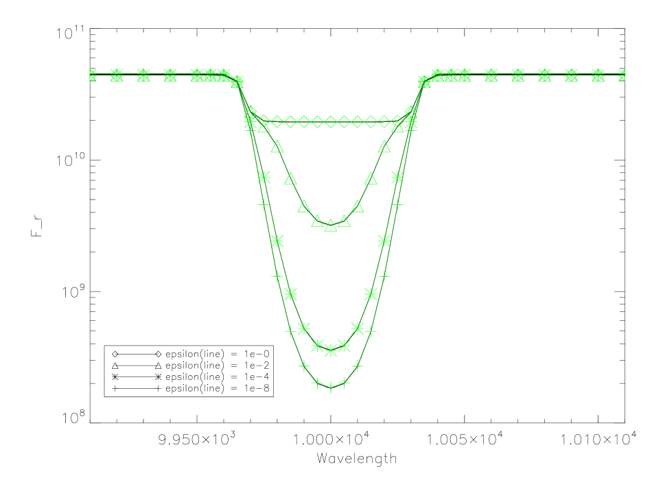
Figure 9: Radial components $F_{r}$ of the flux vectors in the outermost voxels for the line transfer tests in spherical coordinates with $\epsilon_{l}=1,10^{-2},10^{-4},10^{-8}$ and $256^{2}$ solid angle points. The results of the 1D calculations are shown for comparison.

In Figs. 7 and 8 we show the flux vectors of the outermost voxels (outermost radius, all $(\theta_{c},\phi_{c})$ points) for the line transfer case with $\epsilon_{l}=1$ and for different numbers of solid angle points. In the test case, the radial component of the flux vector $F_{r}$ should be the only non-zero component as in spherical symmetry both $F_{\theta}$ and $F_{\phi}$ are zero. The figures show that this is indeed the case if a large enough number of solid angle points is used in the calculation, if the number is too small, $F_{\theta}$ and $F_{\phi}$ can have errors of about 10% and $F_{r}$ scatters considerably around the 1D comparison. For $512^{2}$ solid angle points, the scatter of $F_{r}$ is too small to be seen in the plot and $F_{\theta}$ and $F_{\phi}$ are smaller than 1% of $F_{r}$ over the whole surface of the spherical grid. This highlights the necessity of having enough solid angle points to obtain good accuracy. Fig. 9 shows $F_{r}$ compared to the 1D results for a number of values of $\epsilon_{l}$. In all cases the results agree very well with each other, showing the good numerical accuracy of the 3D code. The results of these tests are valid only for the test cases, therefore, a similar test should be performed for each “real” 3D configuration individually in order to make sure that enough solid angles are used for the accuracy requirements of each individual problem.

With 512 MPI processes on the SGI ICE system of the HLRN the line test with $\epsilon_{l}=10^{-4}$ and $n_{r}=n_{\phi}=65$ and $n_{\theta}=33$ spatial points, $32$ wavelength points and $256^{2}$ solid angle points requires 30 iterations and 20287 s wallclock time and for the same case with $64^{2}$ solid angles the total wallclock time is 1400 s. In both cases we used 32 “clusters” with 16 MPI processes each so that for each wavelength 16 MPI processes work on a formal solution (see paper II for details).

4 Cylindrical coordinates

The setup for the test of the code in cylindrical coordinates is essentially identical to the tests of the spherical coordinate system version. However, describing a spherically symmetric objects in cylindrical coordinates is non-optimal and we expect results comparable to those presented in papers I and II. The cylindrical coordinate system version of the code allows for different maps in $\rho$ and $z$ for flexibility describing objects with nearly cylindrical symmetry.

The differences in the basic setup compared to the spherical coordinates tests are

1. inner radius $r_{c}=10^{10}\,$cm, outer radius $\hbox{$r_{\rm out}$}=11\times 10^{10}\,$cm.

2. linear radial grid.

3. Continuum extinction $\chi_{c}=C/r^{5}$, with the constant $C$ fixed by the radius and optical depth grids, for the continuum tests, $\chi_{c}=C$ for the line transfer tests.

All other test parameters are the same as above.

4.1 Results

For the cylindrical coordinate tests we show just the results of a standard test discussed in Paper I and above for the spherical case with $\epsilon=10^{-2}$. The results for the continuum test case are presented in Fig. 10. The results agree reasonably well with the 1D test case, comparable to the results described in Paper I. The reason for this is that describing a sphere in cylindrical coordinates is not an ideal use of this coordinate system, therefore much higher grid resolution is required to reach reasonable accuracy (the results for grids with $n_{\rho}=n_{\theta}=n_{z}=64$ are substantially worse). As for the test cases in spherical coordinates the resolution in solid angles is very important for accurate results. The convergence behavior is the same as in the case of spherical coordinates.

5 Conclusions

We have discussed the extension of our 3D framework to 3D spherical and cylindrical coordinate systems. These coordinates are better suited than Cartesian coordinates for problems that are approximately spherical (e.g., supernova envelopes) or cylindrical (e.g., protoplanetary disks). The convergence properties and the accuracy of the solutions are comparable to the 1D solution for the test cases discussed here. These additional coordinate systems allow for more general use with higher internal accuracy while using less memory than the purely Cartesian coordinate system.

The next step in the development of the 3D framework is to add the treatment of velocity fields in the observer’s frame and the co-moving frame. The latter will be important for applications with relativistic velocity fields, e.g., supernovae, while the former is interesting for modeling the spectra of convective flow models.

Figure 4: Convergence behavior for the ’large’ continuum test case in spherical coordinates with $\epsilon_{c}=10^{-4}$ for various combinations of local/non-local ${\Lambda^{*}}$ and Ng acceleration. ’NN’ indicates the non-local nearest neighbor ${\Lambda^{*}}$ operator, ’diagonal’ the local ${\Lambda^{*}}$. For comparison the results for the 1D spherical code and the 3D lambda iterations are also plotted.

Figure 7: Flux vectors in the outermost voxels for the line transfer test in spherical coordinates with $\epsilon_{l}=1$ and $64^{2}$ solid angle points. The top panel shows the radial component $F_{r}$ of the voxel flux vector compared to the results for the 1D comparison calculation. The middle and bottom panels show the ratio of the polar $F_{\theta}$ and azimuthal $F_{\phi}$ flux components to $F_{r}$, respectively.

Figure 10: Results for an example of a grey radiative transfer calculation for a sphere in cylindrical 3D coordinates for $\epsilon=10^{-2}$ with $n_{\rho}=n_{\theta}=n_{z}=64$ and $64^{2}$ solid angle points. The results of the 1D calculations are shown for comparison with $*$ symbols.