Counting states in the
Bousso-Polchinski Landscape

Abstract

Starting from an exact counting of small and positive cosmological constant states in the Bousso-Polchinski Landscape we recover a well-known approximate formula and a systematic method of improvement by means of the Poisson summation formula. This is a contribution to the special Volume published by the University of Zaragoza in honor of Julio Abad Antoñanzas. En memoria de nuestro amigo, compañero y maestro Julio.

Bousso-Polchinski Landscape, Cosmological Constant 04.60.-m,11.25.-w

1 Introduction

One of the recent proposals to solve the cosmological constant problem in cosmology is provided by string theory. By dimensional reduction from M-theory to 3+1 dimensions, vacua of the effective theory are classified by means of a big number of quantized fluxes leading to an enormous amount of metastable vacua, the Bousso-Polchinski (BP) Landscape [1]. The cosmological constant problem, namely the smallness of the observed vacuum energy density in the universe [2, 3], can be solved by the presence in this model of a huge number of states of very small, positive cosmological constant, together with a dynamical mechanism given by eternal inflation [4] which allows the system to visit all the vacua. An anthropic selection is then advocated to explain the smallness of the observed cosmological constant [5, 6].

In order to quantify this selection a counting of accesible states in the Landscape is needed. The simplest one is the Bousso-Polchinski count, which computes the volume of a spherical shell of small thickness in flux space and divides it by the volume of a cell. We will now briefly review this argument (see [1]).

A vacuum of the BP Landscape is a node in a $J$-dimensional lattice ${\cal L}$ generated by $J$ charges $q_{1},\cdots,q_{J}$ determined by the sizes of the three-cycles in the compactification manifold. The lattice ${\cal L}$ is

$$\mathcal{L}=\bigl{\{}(n_{1}q_{1},\cdots,n_{J}q_{J})\in\Rset^{J}\colon n_{1},\cdots,n_{J}\in\Zset\bigr{\}}\,.$$ (1)

The $j$-th coordinate of a point in the lattice is an integer multiple of the charge $q_{j}$, and therefore a vacuum is characterized by the integer $J$-tuple $n=(n_{1},\cdots,n_{J})$.

A fundamental cell (also called Voronoi cell) $Q_{n}$ around a node $n$ in a lattice ${\cal L}$ is the subset of $\Rset^{J}$ which contains the points which are closer to $n$ than to any other node of ${\cal L}$. Thanks to the discrete translational symmetry of our lattice (1), all fundamental cells in ${\cal L}$ are translates of the fundamental cell around the origin $Q_{O}\equiv Q$, which we can parametrize in Cartesian coordinates as a product of symmetric intervals

$$Q=\prod_{j=1}^{J}\Bigl{[}-\frac{q_{j}}{2},\frac{q_{j}}{2}\Bigr{]}\,.$$ (2)

The cosmological constant of vacuum $n$ in the BP model is

$$\Lambda(n)=\Lambda_{0}+\frac{1}{2}\sum_{j=1}^{J}n_{j}^{2}q_{j}^{2}\,.$$ (3)

In (3), $\Lambda_{0}$ is an a priori cosmological constant or order $-1$. Each value of $\Lambda>\Lambda_{0}$ defines a spherical ball on the $J$-dimensional flux space of radius $R_{\Lambda}=\sqrt{2(\Lambda-\Lambda_{0})}$. We call this ball ${\cal B}^{J}(\Lambda)$. We take small values of the charges $q_{j}$ (natural values expected by BP are of order $\frac{1}{6}$) in such a way that the ball can contain a huge number of fundamental cells.

The number of states in the Weinberg Window, that is the range of values of the cosmological constant allowing the formation of structures (like galaxies) needed for the formation of life as we know it [6], is obtained by computing the volume of a thin spherical shell in flux space (the realization in the BP Landscape of the Weinberg Window) divided by the volume of a cell in the lattice:

$$\begin{split}\mathcal{N}_{\text{WW}}&=\frac{\mathop{\rm vol}{\cal B}^{J}(\Lambda_{\text{WW}})-\mathop{\rm vol}{\cal B}^{J}(0)}{\mathop{\rm vol}Q}\approx\frac{1}{\mathop{\rm vol}Q}\left.\frac{\,{\rm d}}{\,{\rm d}\Lambda}\Bigl{(}\mathop{\rm vol}{\cal B}^{J}(\Lambda)\Bigr{)}\right|_{\Lambda=0}\Lambda_{\text{WW}}\\ &=\frac{1}{\mathop{\rm vol}Q}\left.\frac{\,{\rm d}}{\,{\rm d}\Lambda}\Bigl{(}\frac{R_{\Lambda}^{J}}{J}\mathop{\rm vol}{S}^{J-1}\Bigr{)}\right|_{\Lambda=0}\Lambda_{\text{WW}}=\mathop{\rm vol}{S}^{J-1}\frac{R_{0}^{J-2}\Lambda_{\text{WW}}}{\mathop{\rm vol}Q}\,,\end{split}$$ (4)

where $R_{0}=R_{\Lambda=0}=\sqrt{2|\Lambda_{0}|}$ (we will call it henceforth $R$), and the volume of the $J-1$ dimensional sphere is

$$\mathop{\rm vol}S^{J-1}=\frac{2\pi^{\frac{J}{2}}}{\Gamma\bigl{(}\frac{J}{2}\bigr{)}}\,.$$ (5)

This method can be naively expected to yield a good estimate when the linear dimensions of the cell are small when compared to the thickness of the shell; but this condition is not satisfied in the BP Landscape. Nevertheless, the result of this counting formula is very good when compared to actual numerical experiments. In the following, we will re-derive the BP count, systematic improvements and a condition of validity.

Our proposal is based on the following kinds of states one may encounter near the null cosmological constant surface in flux space:

• Boundary (or penultimate after Bousso and Yang [7]) are those states in which a Brown-Teitelboim [8, 9] decay chain can end before jumping into the negative cosmological constant sea. So we define a boundary state as one having

  • positive cosmological constant, and

  • at least one neighbor of negative cosmological constant.

• Secant states have the property that their Voronoi cells in flux space have non-empty intersection with the null cosmological constant surface in flux space. Note that a secant state may have negative cosmological constant.

These two categories are not equivalent; a boundary state may not be secant if it is far enough from the null cosmological constant surface, and a secant state may not be boundary if it has negative cosmological constant. So we are interested mainly in the states which are both secant and boundary, because all the states in the Weinberg Window are in this category.

Our strategy will be as follows. We will count the states in the Weinberg Window using the secant states instead of the boundary states. We approximate the exact count using the Poisson summation formula in section 2. The same technique is used to obtain a distribution of values of the cosmological constant and the number of states in the Weinberg Window in section 3. Our results yield the BP count as the lowest order approximation as well as systematic improvements. In section 4 we sketch the difficulties encountered while extending the method to the boundary states. Finally, we summarize the conclusions in section 5.

This work is a continuation of the counting method introduced in [10].

2 Counting secant states

If $\lambda=(n_{1}q_{q},\cdots,n_{J}q_{J})$ is a secant state of the lattice $\mathcal{L}$, the $\Lambda=0$ sphere intersects its Voronoi cell. The line which links the origin with $\lambda$ hits the sphere in a single point, $z$. The directions of $\lambda$ and $z$ are the same, $\upsilon\in S^{J-1}$, and their norms are $\|z\|=R$ and $\|\lambda\|=R+\rho$. The parameter $\rho$ is simply the distance between the sphere and $\lambda$ (see figure 1), and has a close relation with the cosmological constant:

$$\rho=\sqrt{2(\Lambda-\Lambda_{0})}-\sqrt{2|\Lambda_{0}|}\,.$$ (6)

In particular, $\Lambda$ is positive if and only if $\rho$ is positive, and $\Lambda=0$ if and only if $\rho=0$.

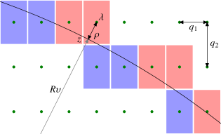
Figure 1: Secant states are shown in a $J=2$ BP model along with the definition of the $\rho$ and $\upsilon$ parameters.

Note that the pair $(\rho,\upsilon)$ determines the tangent hyperplane on the $\Lambda=0$ sphere at $z$, and therefore can be identified with this hyperplane $h=(\rho,\upsilon)$. Note that $h$ intersects the Voronoi cell of $\lambda$, but $z$ is not necessarily inside the cell. The set of possible $z$ points, each corresponding to a secant hyperplane, can be specified by computing the maximum value which $\rho$ can have for a fixed direction $\upsilon$. We will call this quantity $\rho_{\text{max}}=\sigma(\upsilon)$, which is given by the distance of the most distant secant hyperplane

$$\upsilon\cdot(x-c_{\upsilon})=0\,,$$ (7)

where $c_{\upsilon}=\frac{1}{2}(s_{1}q_{1},\cdots,s_{J}q_{J})$ is the unique corner out of $2^{J}$ which belongs to the same $J$-quadrant as $\upsilon$, and the $s_{j}$ are signs $\pm 1$, indeed the same signs of the components of $\upsilon$. We find

$$\sigma(\upsilon)=\upsilon\cdot c_{\upsilon}=\frac{1}{2}\sum^{J}_{j=1}q_{j}s_{j}^{2}|\upsilon_{j}|=\frac{1}{2}\sum^{J}_{j=1}q_{j}|\upsilon_{j}|=\frac{1}{2}q\cdot|\upsilon|\,.$$ (8)

In (8), $|\upsilon|=(|\upsilon_{1}|,\cdots,|\upsilon_{J}|)$. Note that the function $\sigma(\upsilon)$ defines a surface in flux space which contains the possible $z$ points, equivalently, the possible secant hyperplanes. We call the interior of this surface the (secant) hyperplane space associated to the cell, $H_{Q}$, and a hyperplane $h=(\rho,\upsilon)$ is in $H_{Q}$ if and only if $\rho\leq\sigma(\upsilon)$.

If we take all secant states of a given lattice and we gather all their cells into one, the $z$ points seem to be randomly distributed inside $H_{Q}$ (see figure 2). So our suggestion is to provide an explicit form for the probability measure which governs this random distribution. We call the choosing of a particular measure $\,{\rm d}P(\rho,\upsilon)$ in $H_{Q}$ a random hyperplane model (RHM).

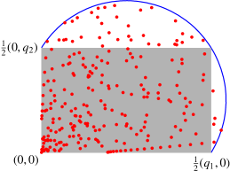
Figure 2: Secant hyperplanes of positive $\rho$ in a $J=2$ BP landscape. Each dot is a $z$ point of a secant state. The shaded region is the first quadrant of the cell $Q$, and all dots lie inside the blue contour, which is the (first quadrant) boundary of hyperplane space $H_{Q}$.

In our previous work [10] we chose the uniform probability measure, and we will justify this assumption as an approximation in section 3.

We start using an exact expression for the number of secant states of positive cosmological constant. We call this number $\mathcal{N}_{S}$. For each secant state $\lambda$, we denote by $\rho(\lambda)$ and $\sigma(\lambda)$ the parameters of its associated secant hyperplane, being simply

$$\rho(\lambda)=\|\lambda\|-R\,,\quad\sigma(\lambda)=\frac{1}{2}q\cdot\frac{|\lambda|}{\|\lambda\|}\,.$$ (9)

Using the restriction $\rho\leq\sigma(\upsilon)$ and the indicator function $\chi_{I}(x)$ of an interval $I\subset\Rset$ (which is 1 if $x\in I$ and 0 otherwise), we can write

$$\mathcal{N}_{S}=\sum_{\lambda\in\mathcal{L}}\chi_{[0,\sigma(\lambda)]}[\rho(\lambda)]\,.$$ (10)

Direct use of (10) is unfeasible; we would have to compile all secant states to count them. But it has the form

$$\sum_{\lambda\in\mathcal{L}}f(\lambda)\quad\text{with}\quad f(x)=\chi_{[0,\sigma(x)]}[\rho(x)]\quad(x\in\Rset^{J})\,,$$ (11)

and therefore we can obtain an alternative representation using the Poisson summation formula:

$$\sum_{\lambda\in\mathcal{L}}f(\lambda)=\frac{1}{\mathop{\rm vol}Q}\sum_{\kappa\in\mathcal{L}^{*}}\hat{f}(\kappa)$$ (12)

where we use the Fourier transform of $f(x)$

$$\hat{f}(\xi)=\int_{\Rset^{J}}f(x)e^{-i\xi\cdot x}\,{\rm d}^{J}x\,,$$ (13)

and the dual lattice of $\mathcal{L}$

$$\mathcal{L}^{*}=\biggl{\{}\biggl{(}m_{1}\frac{2\pi}{q_{1}},\cdots,m_{J}\frac{2\pi}{q_{J}}\biggl{)}\in\Rset^{J}\colon m_{1},\cdots,m_{J}\in\Zset\biggr{\}}\,,$$ (14)

determined by the condition $e^{i\lambda\cdot\kappa}=1$. In fig. 3 a $J=2$ lattice and its dual are shown.

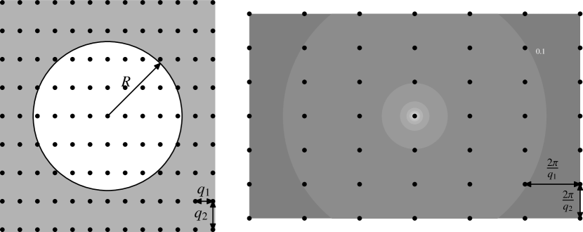
Figure 3: $J=2$ lattice with a typical scale $R$ (left). Dual lattice (right). The shaded circles show decreasing amplitude of the envelope of the Bessel function $J_{0}(R\|\xi\|)$, which is the Fourier transform of the normalized indicator function of the circle of radius $R$ in the former lattice. The 0.1 label signals the distance in dual space where the amplitude at the origin is reduced to 1/10.

In order to use eq. (12) we need to compute

$$\hat{f}(\xi)=\int_{\Rset^{J}}\chi_{[0,\sigma(x)]}[\rho(x)]e^{-i\xi\cdot x}\,{\rm d}^{J}x\,.$$ (15)

Switching to spherical variables and then using $\rho$ as integration variable, we obtain

$$\hat{f}(\xi)=\int_{S^{J-1}}\,{\rm d}\Omega_{J-1}(\upsilon)\,e^{-iR(\xi\cdot\upsilon)}\int^{\sigma(\upsilon)}_{0}(\rho+R)^{J-1}e^{-i\rho(\xi\cdot\upsilon)}\,{\rm d}\rho\,.$$ (16)

Exact evaluation of this integral is difficult, as might be expected. The lowest order approximation in (12) yields the following formula for the number of positive $\Lambda$ secant states:

$$\mathcal{N}_{S}=\frac{\hat{f}(0)}{\mathop{\rm vol}Q}=\frac{1}{\mathop{\rm vol}Q}\int_{S^{J-1}}\,{\rm d}\Omega_{J-1}(\upsilon)\,\int^{\sigma(\upsilon)}_{0}(\rho+R)^{J-1}\,{\rm d}\rho\,.$$ (17)

We can expect this to be an accurate approximation from the following qualitative argument. The function $f(x)$ is supported at a compact domain whose extent is proportional to some average charge $\overline{q}$ times a $J$-dependent constant. The Fourier transform $\hat{f}(\xi)$ will be then concentrated at a domain of dimensions proportional to $1/\overline{q}$. But the spacings between neighboring nodes of the dual lattice are the inverses of the charges, and thus only a few of these nodes will enter the domain with significant amplitude.

In this approximation, we can rewrite eq. (17) as

$$\frac{1}{\mathcal{N}_{S}\mathop{\rm vol}Q}\int_{S^{J-1}}\,{\rm d}\Omega_{J-1}(\upsilon)\,\int^{\sigma(\upsilon)}_{0}(\rho+R)^{J-1}\,{\rm d}\rho=1\,,$$ (18)

which asserts that the following probability measure is normalized:

$$\,{\rm d}P(\rho,\upsilon)=\chi_{[0,\sigma(\upsilon)]}(\rho)\frac{(\rho+R)^{J-1}\,{\rm d}\rho\,{\rm d}\Omega_{J-1}(\upsilon)}{\mathcal{N}_{S}\mathop{\rm vol}Q}\,.$$ (19)

The $\chi$ function simply restricts the range of integration to the secant hyperplane set $H_{Q}$. The previous measure can be expressed using the $z$ points mentioned above translated to a single cell $Q$, that is, considering $z\mod{\mathcal{L}}$, the measure (19) is

$$\,{\rm d}P(z)=\chi_{H_{Q}}(z)\frac{\,{\rm d}^{J}z}{\mathcal{N}_{S}\mathop{\rm vol}Q}\,,$$ (20)

that is, the uniform probability in $H_{Q}$. So the random hyperplane model obtained to the lowest order in the Poisson summation formula is simply the uniform probability measure over $H_{Q}$. This is the choice we made in [10].

Integrating out the $\rho$ variable in (17) we find

$$\begin{split}\mathcal{N}_{S}&=\frac{1}{J\mathop{\rm vol}Q}\int_{S^{J-1}}\bigl{[}(R+\sigma(\upsilon)\bigr{)}^{J}-R^{J}\bigr{]}\,{\rm d}\Omega_{J-1}(\upsilon)\\ &=\frac{1}{J\mathop{\rm vol}Q}\sum^{J}_{k=1}\binom{J}{k}R^{J-k}\int_{S^{J-1}}\sigma(\upsilon)^{k}\,{\rm d}\Omega_{J-1}(\upsilon)\,.\end{split}$$ (21)

The first term in this expansion can be computed exactly (this is done in [10]):

$$\int_{S^{J-1}}\sigma(\upsilon)\,{\rm d}\Omega_{J-1}(\upsilon)=\frac{\mathop{\rm vol}S^{J-2}}{J-1}\sum^{J}_{j=1}q_{j}\,,$$ (22)

so that we recover the formula obtained in [10] with a completely different approach:

$$\mathcal{N}_{S}=\frac{\mathop{\rm vol}S^{J-2}}{J-1}\,\frac{R^{J-1}}{\mathop{\rm vol}Q}\sum^{J}_{j=1}q_{j}\,.$$ (23)

Note the absence of a factor 2 here because of the counting of positive $\Lambda$ states only.

The validity condition of formula (23) is

$$\sigma(\upsilon)\leq\sigma_{\text{max}}=\frac{1}{2}\sqrt{\sum^{J}_{j=1}q_{j}^{2}}\lll R\,.$$ (24)

Using a mean square charge $\tilde{q}^{2}=\frac{1}{J}\sum^{J}_{j=1}q_{j}^{2}$, condition (24) can be rewritten as

$$J\frac{\tilde{q}^{2}}{|\Lambda_{0}|}\lll 8\,.$$ (25)

3 Number of states in the Weinberg Window

We can follow the same steps for the number of states of very low cosmological constant. If $\Lambda_{\text{WW}}$ is a very small number characterizing the anthropic range (which comprises the experimental value $\Lambda_{\text{exp}}\approx 10^{-123}$), we will call $\rho_{a}$ the corresponding value of the $\rho$ parameter computed using eq. (6), that is

$$\rho_{a}=\sqrt{2(\Lambda_{\text{WW}}-\Lambda_{0})}-\sqrt{2|\Lambda_{0}|}\approx\frac{\Lambda_{\text{WW}}}{R}\,.$$ (26)

The number of states in the BP lattice having $0\leq\rho(\lambda)\leq\tau$ for fixed $\tau$ is

$$\Omega(\tau)=\sum_{\lambda\in\mathcal{L}}\chi_{[0,\sigma(\lambda)]\cap[0,\tau]}[\rho(\lambda)]\,.$$ (27)

Note that $\Omega(\tau)=\mathcal{N}_{S}$ if $\tau>\sigma_{\text{max}}$, so that interpreting each secant state as a random equiprobable event we obtain the general formula

$$\Omega(\tau)=\mathcal{N}_{S}P(0\leq\rho\leq\tau)\,.$$ (28)

On the other hand, if $\tau<\frac{1}{2}\min_{j}\{q_{j}\}=\sigma_{\text{max}}$, then $[0,\sigma(\lambda)]\cap[0,\tau]=[0,\tau]$ and we have $f(x)=\chi_{[0,\tau]}[\rho(x)]$, which simplifies the Fourier transform (16) to

$$\hat{f}(\xi)=\int_{S^{J-1}}\,{\rm d}\Omega_{J-1}(\upsilon)\,e^{-iR(\xi\cdot\upsilon)}\int^{\tau}_{0}(\rho+R)^{J-1}e^{-i\rho(\xi\cdot\upsilon)}\,{\rm d}\rho\,.$$ (29)

For $\tau$ as small as $\rho_{a}$, a first order Taylor expansion around $\tau=0$ yields

$$\hat{f}(\xi)=R^{J-1}\tau\int_{S^{J-1}}\,{\rm d}\Omega_{J-1}(\upsilon)\,e^{-iR(\xi\cdot\upsilon)}\,.$$ (30)

Taking only the first term in the Poisson summation formula we obtain

$$\Omega(\tau)\approx\frac{\hat{f}(0)}{\mathop{\rm vol}Q}=\frac{R^{J-1}}{\mathop{\rm vol}Q}\,\mathop{\rm vol}S^{J-1}\,\tau\,,$$ (31)

which is the number of states in the Weinberg Window once we specialize $\tau=\rho_{a}=\frac{\Lambda_{\text{WW}}}{R}$ in equation (31):

$$\mathcal{N}_{\text{WW}}=\frac{R^{J-2}}{\mathop{\rm vol}Q}\,\mathop{\rm vol}S^{J-1}\,\Lambda_{\text{WW}}\,.$$ (32)

This formula is exactly the Bousso-Polchinski count given in [1] and rederived in [10] using the RHM.

It turns out that the Fourier transform (30) can be given in closed form, allowing systematic improvements to be added to (32). To show this, we rewrite (30) as

$$\hat{f}(\xi)=R^{J-1}\tau\int_{S^{J-1}}\,{\rm d}\Omega_{J-1}(\upsilon)\,e^{-iR(\xi\cdot\upsilon)}=\tau\frac{\partial}{\partial R}\int_{\Rset^{J}}\theta(R^{2}-\|x\|^{2})\,e^{-i\xi\cdot x}\,{\rm d}^{J}x\,.$$ (33)

Now, we use the following integral representation for the $\theta$ function:

$$\theta(t)=\frac{1}{2\pi i}\int_{\gamma}\frac{e^{st}}{s}\,{\rm d}s\,,$$ (34)

where $\gamma$ is a contour running from $c-i\infty$ to $c+i\infty$ for real $c$ located to the right side of all singularities of the integrand. We have

$$\begin{split}\hat{f}(\xi)&=\frac{\tau}{2\pi i}\int_{\gamma}\frac{\,{\rm d}s}{s}\frac{\partial}{\partial R}\int_{\Rset^{J}}e^{s(R^{2}-\|x\|^{2})-i\xi\cdot x}\,{\rm d}^{J}x\\ &=\frac{2R\tau}{2\pi i}\int_{\gamma}e^{sR^{2}}\,{\rm d}s\prod^{J}_{j=1}\int_{\Rset}e^{-sx_{j}^{2}-i\xi_{j}x_{j}}\,{\rm d}x_{j}\\ &=\frac{2R\tau}{2\pi i}\int_{\gamma}e^{sR^{2}}\,{\rm d}s\prod^{J}_{j=1}\sqrt{\frac{\pi}{s}}\,e^{-\frac{\xi_{j}^{2}}{4s}}\\ &=\frac{2R\tau\pi^{\frac{J}{2}}}{2\pi i}\int_{\gamma}e^{sR^{2}-\frac{\|\xi\|^{2}}{4s}}\frac{\,{\rm d}s}{s^{\frac{J}{2}}}\\ &=2R\tau\pi^{\frac{J}{2}}\biggl{(}\frac{2R}{\|\xi\|}\biggr{)}^{\frac{J}{2}-1}J_{\frac{J}{2}-1}(R\|\xi\|)\,.\end{split}$$ (35)

The last step is an inverse Laplace transform resulting in a Bessel function. Let us write this result in a slightly more convenient form, using $\nu=\frac{J}{2}-1$:

$$\hat{f}(\xi)=R\tau\,R^{J-2}\frac{2\pi^{\frac{J}{2}}}{\Gamma\bigl{(}\frac{J}{2}\bigr{)}}L_{\nu}(R\|\xi\|)\,,\quad\text{with}\quad L_{\nu}(t)=\Gamma(\nu+1)2^{\nu}\frac{J_{\nu}(t)}{t^{\nu}}\,.$$ (36)

The function $L_{\nu}(t)$ satisfies $L_{\nu}(0)=1$ and has a gaussian shape near $t=0$, $L_{\nu}(t)\approx e^{-\frac{t^{2}}{4(\nu+1)}}$, followed by a regime of damped oscillations with an envelope proportional to $t^{-\nu-\frac{1}{2}}$. We can use this expression to write the first correction to (32) by choosing the $2J$ neighbors of the origin in the dual lattice. For these, $\|\xi\|=\frac{2\pi}{q_{j}}$ for each axis, so we have

$$\mathcal{N}_{\text{WW}}=\Lambda_{\text{WW}}\frac{R^{J-2}}{\mathop{\rm vol}Q}\,\mathop{\rm vol}S^{J-1}\,\biggl{[}1+2\sum^{J}_{j=1}L_{\nu}(2\pi R/q_{j})\biggr{]}\,.$$ (37)

The first correction will be small when compared to (32) if

$$2\biggl{|}\sum^{J}_{j=1}L_{\nu}(2\pi R/q_{j})\biggr{|}\ll 1\,.$$ (38)

Condition (38) will be satisfied as long as the $J$ numbers $2\pi\frac{R}{q_{j}}$ are scattered along regions of different sign of the Bessel function, allowing a huge cancellation in the sum. The worst case will occur when all charges are equal (let $q$ be their common value), and then we must demand that $2\pi\frac{R}{q}$ is very far from the gaussian regime of the function $L_{\nu}(t)$, that is,

$$2\pi\frac{R}{q}\gg k\sqrt{J}\quad\Rightarrow\quad J\frac{q^{2}}{|\Lambda_{0}|}\ll\frac{8\pi^{2}}{k}\,,$$ (39)

where the number $k$ is $J$-dependent. For $J=2$ ($\nu=0$), taking $10^{-2}$ as a reference amplitude for a relative error of $1\%$, we need a value of $k\sqrt{2}$ large enough to be in the asymptotic regime of the Bessel function, so we have

$$4\sqrt{\frac{2}{\pi k\sqrt{2}}}=10^{-2}\quad\Rightarrow\quad k\approx 72025.3\,,$$ (40)

which implies $q\ll 0.01655R$ from (39), but for $J=22$ ($\nu=10$) the value $10^{-2}$ is in the gaussian regime, and we have

$$44e^{-\frac{k^{2}}{2}}=10^{-2}\quad\Rightarrow\quad k\approx 4.09618\,,$$ (41)

which implies $q\ll 0.66188R$. We see that the requirements in the charges are not too restrictive so that the Bousso-Polchinki count (32) can be reasonably accurate.

We can also expect the subsequent corrections to be small when compared to the first one because of the cancellations in the sum of Bessel functions.

4 Replacing secant by boundary states

If we want to use boundary states to count the low-$\Lambda$ states, we must find a condition satisfied by them which is analogous to $\rho<\sigma(\upsilon)$ for the secant states. A boundary state has positive $\Lambda$ but some neighbors (possibly only one) of negative $\Lambda$, which means that the $\Lambda=0$ sphere must cut the segment joining both states. The segments joining a boundary state with its $2J$ neighbors constitute the skeleton of a cell which have these neighbors as vertices and a face for each “$J$-quadrant” determined by the $J$ vertices in it. For $J=2$, such a cell is simply a rhombus with the neighbors at its corners, and for $J=3$ the cell is an octahedron. We will call this cell a $J$-rhombus.

These cells are not disjoint, and do not cover the whole flux space, so we cannot use them for tessellate flux space in order to count states naively. But we can reformulate the condition of a boundary state as being secant with respect to this cell instead of its Voronoi cell. Note that the $\Lambda=0$ surface intersecting a $J$-rhombus will have its $\rho$ and $\upsilon$ parameters defined, so the boundary condition is again $\rho<\sigma(\upsilon)$ for a different $\sigma$ interpreted as the boundary of the space of hyperplanes associated to boundary states.

Again, $\sigma(\upsilon)$ is the maximum distance that a hyperplane associated to a boundary state (“boundary hyperplane” henceforth) can reach in a given direction $\upsilon$. The distance will be maximum if the hyperplane contains at least one vertex of the $J$-rhombus. If we assume the center of the $J$-rhombus to be at the origin, the vertices are the points $s_{i}q_{i}e_{i}$, where $s_{i}=\pm 1$ and $e_{i}$ is the unit vector of the $i^{\text{th}}$ axis. The equation of a maximum distance boundary hyperplane is

$$v\cdot(x-s_{i}q_{i}e_{i})=0\,,$$ (42)

so that the maximum distance is $\sigma(\upsilon)=|\upsilon_{i}|q_{i}$. The value of $i$ and $s_{i}$ are chosen in the following way. Let $u$ be the normal unit vector to the face of the $J$-rhombus in the first (all positive components) $J$-quadrant, $S^{J-1}_{+}$:

$$u=\frac{(q_{1}^{-1},\cdots,q_{J}^{-1})}{\sum^{J}_{j=1}q_{j}^{-2}}\,.$$ (43)

Point $u$ decomposes $S^{J-1}_{+}$ in the following $J$ regions:

$$\Xi_{i}=\Bigl{\{}\upsilon\in S^{J-1}_{+}\colon\upsilon_{i}\geq u_{i},\ {}\upsilon_{j}\leq u_{j}\quad\text{for $j\neq i$}\Bigr{\}}\,.$$ (44)

Now, let us move $\upsilon$ to $S^{J-1}_{+}$ by removing the signs: $|\upsilon|=(|\upsilon_{1}|,\cdots,|\upsilon_{J}|)$. Choose the label $i$ for the set $\Xi_{i}$ which $\upsilon$ belongs to, and choose the sign $s_{i}$ to be that of $\upsilon_{i}$. Thus, we find

$$\sigma(\upsilon)=\sum^{J}_{i=1}q_{i}|\upsilon_{i}|\chi_{\Xi_{i}}(|\upsilon|)\,.$$ (45)

For $J=2$ we have $u\propto(\frac{1}{q_{1}},\frac{1}{q_{2}})$ and this determines an angle $\theta_{0}=\tan^{-1}\frac{q_{1}}{q_{2}}$. $\Xi_{1}$ comprises the directions $\upsilon=(\cos\theta,\sin\theta)$ for which $\theta\leq\theta_{0}$ and $\Xi_{2}$ the converse $\theta\geq\theta_{0}$. An example of this boundary is shown in figure 4.

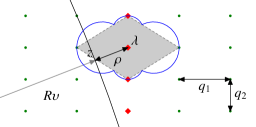
Figure 4: Boundary states (diamonds) in a $J=2$ BP lanscape. The shaded region is the $2$-rhombus. The boundary of the boundary hyperplane space is also displayed. Note that the $z$ point is slightly outside the rhombic cell.

Once the $\sigma$ function has been found, we can write a formula analogous to (21) for the number of boundary states, whose first term is

$$\mathcal{N}_{B}=\frac{R^{J-1}}{\mathop{\rm vol}Q}\int_{S^{J-1}}\sigma(\upsilon)\,{\rm d}\Omega_{J-1}(\upsilon)\,.$$ (46)

The validity condition now is

$$\sigma(\upsilon)\leq\sigma_{\text{max}}=\max_{1\leq j\leq J}\{q_{j}\}\lll R\,.$$ (47)

But we do not need to evaluate formula (46) if we only want to count states in the Weinberg Window. Note that equation (27) does not involve $\sigma$ because of the smallness of the shell width, and therefore the number $\mathcal{N}_{\text{WW}}$ computed in section 3 remains unchanged. Only a difference must be stressed in this regard: the shell width must be smaller than the minimum distance $\sigma_{\text{min}}$, which now depends on $J$. It is simply the distance to the cell center of one of its faces. The face at $S^{J-1}_{+}$ has equation $\sum^{J}_{j=1}\frac{x_{j}}{q_{j}}=1$ or $u\cdot x=\sigma_{\text{min}}$, so we have the condition

$$\sigma_{\text{min}}=\biggl{[}\sum^{J}_{j=1}q_{j}^{-2}\biggr{]}^{-\frac{1}{2}}=\frac{\widetilde{q}}{\sqrt{J}}\gg\rho_{a}=\frac{\Lambda_{\text{WW}}}{R}\,,$$ (48)

where $\widetilde{q}$ is a “square-harmonic” average of the charges. Note that this condition is met for natural values of the charges and dimension $J$, so that considering secant or boundary states may change the probability distribution of $\Lambda$ in equation (28) but it has no effect on the number of states in the Weinberg Window.

5 Conclusion

We have developed a general method for counting low-lying states in the Bousso-Polchinki Landscape with the help of the Poisson summation formula without any statistical validation of the assumptions made. This approach provides a firm foundation of the random hyperplane model previously used by the authors. It also allows us to derive validity conditions as well as systematic improvements, and can be used in different problems which can be formulated on a lattice in flux space. Furthermore, the validity condition (48) relates an experimental quantity (the cosmological constant) to a microscopic one (an average charge). We believe that this relation can be pursued in this context.

We would like to thank Concepción Orna for carefully reading this manuscript. This work has been supported by CICYT (grant FPA-2006-02315) and DGIID-DGA (grant 2007-E24/2).

References

- [1] R. Bousso and J. Polchinski: Quantization of four-form fluxes and dynamical neutralization of the cosmological constant. JHEP 06, 006 (2000) [hep-th/0004134].
- [2] S. Weinberg: The cosmological constant problem. Rev. Mod. Phys. 61, 1-23 (1989).
- [3] R. Bousso: TASI Lectures on the Cosmological Constant. Gen. Rel. Grav. 40 (2008) 607 [0708.4231 [hep-th]].
- [4] A. H. Guth: Inflation and Eternal Inflation. Phys. Rept. 333 (2000) 555 and references therein [astro-ph/0002156].
- [5] L. Susskind: The Anthropic Landscape of String Theory. [hep-th/0302219].
- [6] S. Weinberg: Anthropic Bound on the Cosmological Constant. Phys. Rev. Lett. 59, 2607-2610 (1987).
- [7] R. Bousso and I. Yang: Landscape predictions from cosmological vacuum selection. Phys. Rev. D 75 (2007) 123520 [hep-th/0703206].
- [8] J. D. Brown and C. Teitelboim: Dynamical neutralization of the cosmological constant. Phys. Lett. B195, 177 (1987).
- [9] J. D. Brown and C. Teitelboim: Neutralization of the cosmological constant by membrane creation. Nucl. Phys. B297, 787-836 (1988).
- [10] C. Asensio and A. Segui: A geometric-probabilistic method for counting low-lying states in the Bousso-Polchinski Landscape. arXiv:0812.3247v2 [hep-th].