Effects of dust abundance on the far-infrared colours of blue compact dwarf galaxies

Abstract

We investigate the FIR properties of a sample of BCDs observed by AKARI. By utilizing the data at wavelengths of $\lambda=65~{}\mu$m, 90 $\mu$m, and 140 $\mu$m, we find that the FIR colours of the BCDs are located at the natural high-temperature extension of those of the Milky Way and the Magellanic Clouds. This implies that the optical properties of dust in BCDs are similar to those in the Milky Way. Indeed, we explain the FIR colours by assuming the same grain optical properties, which may be appropriate for amorphous dust grains, and the same size distribution as those adopted for the Milky Way dust. Since both interstellar radiation field and dust optical depth affect the dust temperature, it is difficult to distinguish which of these two physical properties is responsible for the change of FIR colours. Then, in order to examine if the dust optical depth plays an important role in determining the dust temperature, we investigate the correlation between FIR colour (dust temperature) and dust-to-gas ratio. We find that the dust temperature tends to be high as the dust-to-gas ratio decreases but that this trend cannot be explained by the effect of dust optical depth. Rather, it indicates a correlation between dust-to-gas ratio and interstellar radiation field. Although the metallicity may also play a role in this correlation, we suggest that the dust optical depth could regulate the star formation activities, which govern the interstellar radiation field. We also mention the importance of submillimetre data in tracing the emission from highly shielded low-temperature dust.

1 Introduction

The far-infrared (FIR) emission from galaxies is often used to trace the star formation activities (Kennicutt, 1998; Inoue et al., 2000; Iglesias-Páramo et al., 2004). Dust grains are the source of FIR emission, and the strong connection between FIR luminosity and star formation rate can be explained if the ultraviolet (UV) light from massive stars is the dominant source of dust heating. The FIR spectral energy distribution (SED) of dust grains reflects various information on the grains themselves and on the sources of grain heating (e.g. , 2003; Takeuchi et al., 2005; Dopita et al., 2005). Dust temperature is determined by the intensity of interstellar radiation field (ISRF) and the optical properties of dust (i.e. how it absorbs and emits light). Since dust grains absorb UV light efficiently, the FIR luminosity and the dust temperature mostly reflect the UV radiation field (Buat & Xu, 1996).

Observationally, dust temperature can be estimated from FIR colour, which is defined as the flux ratio between two FIR wavelengths. If more than two ($\geq 3$) bands are available in FIR, we can take two independent FIR colours and examine a FIR colour–colour relation. A colour–colour relation, because of increased information compared with a single FIR colour, enables us to obtain not only the dust temperature but also the wavelength dependence of dust emissivity. Nagata et al. (2002), adopting 60 $\mu$m, 100 $\mu$m, and 140 $\mu$m as three wavelengths, show that there is a tight relation in the FIR colour–colour diagram. This tightness implies a common wavelength dependence of FIR emissivity among various galaxies. Their work has been developed by Hibi et al. (2006), who show that a tight FIR colour–colour relation found for the Milky Way dust emission, called “main correlation”, is also consistent with the FIR colour–colour relation of a sample of nearby galaxies (see also Sakon et al. 2004; Onaka et al. 2007). As stated by Hibi et al. (2006), this implies that the optical properties of grains in FIR are common among the Milky Way and nearby galaxies.

Since the FIR colour–colour relation can be used to constrain the optical properties of dust grains, the FIR colour–colour relation of galaxies with various evolutionary stages provides pieces of information on the grain evolution in galactic environments. In particular, the dominant production source of dust grain could be different in early phase of galaxy evolution (Todini & Ferrara, 2001; Nozawa et al., 2003; Maiolino et al., 2004; Schneider, Ferrara, & Salvaterra, 2004). Moreover, the effects of interstellar processing of dust grains, especially accretion of heavy elements onto dust grains, coagulation, and shattering, depend on metallicity (or dust abundance). Thus, it is probable that the grain properties evolve as galaxies evolve.

Although it is difficult to obtain the rest-frame FIR data of distant galaxies in an early phase of galaxy evolution, there are nearby possible “templates” of primeval galaxies, blue compact dwarf galaxies (BCDs). Indeed, BCDs have on-going star formation in metal-poor and gas-rich environments (Sargent & Searle, 1970; van Zee, Skillman, & Salzer, 1998), which could be similar to those in high-redshift star-forming galaxies. Moreover, BCDs harbour an appreciable amount of dust (e.g. Thuan, Sauvage, & Madden, 1999) and can be used to investigate the dust properties in chemically unevolved galaxies (Takeuchi et al., 2005).

It is possible to investigate the metallicity dependence of dust properties by sampling BCDs with a variety of metallicity. Recently Engelbracht et al. (2008) have examined the metallicity dependence of dust emission in various wavelengths by using Spitzer data. In FIR, they have used Multiband Imaging Photometer for Spitzer (MIPS) 70 $\mu$m and 160 $\mu$m bands, and have shown that there is a correlation between dust temperature derived from these two bands and metallicity. This indicates the importance of studies on dust emission in a wide metallicity range.

The AKARI satellite (Murakami et al., 2007) provides us with a good opportunity to study FIR colour–colour relations, since Far-Infrared Surveyor (FIS) on AKARI has four bands in FIR (65 $\mu$m, 90 $\mu$m, 140 $\mu$m, and 160 $\mu$m) (Murakami et al., 2007; Kawada et al., 2007). Indeed, seven of the eight BCDs in Hirashita et al. (2008, hereafter H08) are detected at 65 $\mu$m, 90 $\mu$m, and 140 $\mu$m. This indicates that it is possible to study the FIR colour–colour relation of BCDs by using AKARI data. In this paper, we add four more BCDs available in the AKARI archive and examine the FIR colour–colour relation of BCDs. Then, we extract information on what determines or regulates the FIR emission in metal-poor environments with the aid of theoretical models for dust emission.

This paper is organized as follows. First, in Section 2, we describe the models of dust emission with a simple radiative transfer recipe. Then, in Section 3, we explain the data analysis of the BCD sample observed by AKARI. In Section 4, we overview the results of the model calculations in comparison with the observational data. In Section 5, we discuss our results, focusing on the relation between FIR colour and dust content. Finally, the conclusion is presented in Section 6.

2 FIR SED Model

We adopt the theoretical framework of Draine & Li (2001) to calculate the SED of dust emission in FIR. The framework has already been described in Hirashita, Hibi, & Shibai (2007, hereafter HHS07), but we modify it to treat BCDs in this paper. Moreover, as described in the last paragraph in Sect. 2.1, we newly include the effect of radiative transfer in a similar way to Galliano et al. (2003). We overview our framework, focusing on the change from HHS07.

2.1 Interstellar radiation field

The stellar SEDs of BCDs are generally harder than those of spiral galaxies (Boselli, Gavazzi, & Sanvito, 2003). Madden et al. (2006) also show a hard stellar radiation field from the observation of mid-infrared emission lines in low-metallicity star-forming galaxies. Thus, we change the SED of ISRF, and adopt the following fitting formula according to the averaged SED of the BCD sample in Boselli et al. (2003):

$$4\pi\lambda J_{\lambda}^{(0)}=\left\{\begin{array}[]{l}0~{}~{}~{}~{}~{}(\lambda_{\mu\mathrm{m}}\leq 0.0912),\\ 3.02\times 10^{-4}\lambda_{\mu\mathrm{m}}^{-1.20}\\ ~{}~{}~{}~{}~{}~{}~{}(0.0912<\lambda_{\mu\mathrm{m}}\leq 0.25),\\ 1.55\times 10^{-3}\times 10^{-3}\lambda_{\mu\mathrm{m}}^{-0.0371}\\ ~{}~{}~{}~{}~{}~{}~{}(0.25<\lambda_{\mu\mathrm{m}}\leq 0.37),\\ 2.39\lambda_{\mu\mathrm{m}}^{7.41}~{}~{}~{}~{}~{}(0.37<\lambda_{\mu\mathrm{m}}\leq 0.4),\\ 4\pi\lambda[W_{1}B_{\lambda}(T_{1})+W_{2}B_{\lambda}(T_{2})]\\ ~{}~{}~{}~{}~{}~{}~{}(0.4<\lambda_{\mu\mathrm{m}}),\end{array}\right.$$ (9)

where $J_{\lambda}^{(0)}$ is the ISRF intensity whose normalization is determined so that the intensity at wavelength $\lambda=0.2~{}\mu$m (almost the centre of the UV range; Buat & Xu 1996) is equal to the solar neighborhood ISRF estimated by Mathis, Mezger, & Panagia (1983) ($4\pi\lambda J_{\lambda}^{(0)}$ is expressed in units of erg cm^-2 s^-1), $\lambda_{\mu\mathrm{m}}$ is the wavelength in units of $\mu$m, $B_{\lambda}(T)$ is the Planck function, $(T_{1},\,T_{2})=(1000,\,4000~{}\mathrm{K})$, and $(W_{1},\,W_{2})=(1.61\times 10^{-15},\,2.90\times 10^{-14})$.

In this paper, we newly include the effect of dust extinction on the ISRF. We simply assume that the ISRF intensity, $J_{\lambda}$, at optical depth $\tau_{\lambda}$ is

$$J_{\lambda}=J_{\lambda}^{(0)}\chi\exp(-\tau_{\lambda})\,,$$ (10)

where $\chi$ is the scaling factor of the ISRF relative to $J_{\lambda}^{(0)}$ and is assumed to be independent of wavelength. For the wavelength dependence of $\tau_{\lambda}$, we assume the Milky Way extinction curve taken from Cardelli, Clayton, & Mathis (Cardelli et al.1989) with $R_{V}=3.1$. Thus, the extinction at any wavelength $\lambda$, $A_{\lambda}$ (in units of magnitude), can be determined if we set a value of $A_{V}$ (extinction at $V$ band). The optical depth can be related with the extinction as $\tau_{\lambda}=A_{V}/1.086$. The following results does not change drastically if we assume an extinction curve appropriate for the Large Magellanic Clouds (LMC) or the Small Magellanic Cloud (SMC), since the detailed shape of UV–optical SED is not important in this paper. Strictly speaking, we treat scattering as effective absorption, and this treatment would overestimate the absorbed energy. Thus, we interpret $A_{V}$ given here as effective absorption optical depth, so that the total energy absorbed by dust in our formulation is equal to the energy that would be absorbed if scattering were properly treated.

Galliano et al. (2003) also adopted a similar treatment, which is valid if dust is distributed in a thin shell surrounding the stars. Such a “screen” geometry enhances the effect of dust extinction (i.e., radiative transfer) in comparison with a mixed geometry between stars and dust. Thus, our models are suitable to examine the extent to which the radiative transfer effects could affect the FIR SEDs.

2.2 Grain properties

We consider silicate and graphite grains in this paper. Since we are interested in the wavelength range appropriate for the AKARI FIS bands ($\lambda\sim 50$–180 $\mu$m; Section 3.1), we neglect polycyclic aromatic hydrocarbons (PAHs), which contribute significantly to the emission at $\lambda\la 20~{}\mu$m (Désert, Boulanger, & Puget, 1990; Dwek et al., 1997; Draine & Li, 2001).

We assume a grain to be spherical with a radius of $a$. The absorption cross section of the grain is expressed as $\pi a^{2}Q_{\mathrm{abs}}(\lambda)$, where $Q_{\mathrm{abs}}(\lambda)$ is called absorption efficiency. We adopt the optical constants of astronomical silicate and graphite for $\lambda<100~{}\mu$m from Draine & Lee (1984) and Weingartner & Draine (2001) and calculate the absorption efficiency by using Mie theory (Bohren & Huffman, 1983). For the absorption efficiency at $\lambda>100~{}\mu$m, we adopt a functional form proposed by Reach et al. (1995):

$$Q_{\mathrm{abs}}(\lambda)=\frac{(\lambda/\lambda_{0})^{-2}}{[1+(\lambda_{1}/\lambda)^{6}]^{1/6}}\,,$$ (11)

which behaves like $\beta=1$ ($Q_{\mathrm{abs}}(\lambda)\propto\lambda^{-\beta}$, where $\beta$ is called emissivity index) for $\lambda\ll\lambda_{1}$ and $\beta=2$ at $\lambda\gg\lambda_{1}$ (see also Bianchi, Davies, & Alton, 1999). We assume that $\lambda_{1}=200~{}\mu$m, following Reach et al. (1995). We set the value of $\lambda_{0}$ so that the continuity of $Q_{\mathrm{abs}}$ at $100~{}\mu$m is satisfied. As shown in HHS07, the wavelength dependence of $Q_{\mathrm{abs}}$ assumed here explains the FIR colour–colour relations of the Milky Way, the LMC and the SMC. Although the absorption efficiency at $\lambda>100~{}\mu$m is modified, we call the grain species “silicate” and “graphite” according to the adopted absorption efficiency at $\lambda<100~{}\mu$m.

The number density of grains with sizes between $a$ and $a+\mathrm{d}a$ is denoted as $n_{i}(a)\,\mathrm{d}a$, where the subscript $i$ denotes a grain species (silicate or graphite). Since there is little knowledge on the grain size distribution in BCDs, we simply assume a power-law form for $n_{i}(a)$:

$$n_{i}(a)=\mathcal{C}_{i}a^{-K}~{}~{}~{}(a_{\mathrm{min}}\leq a\leq a_{\mathrm{max}})\,,$$ (12)

where $a_{\mathrm{min}}$ and $a_{\mathrm{max}}$ are the upper and lower cutoffs of grain size, respectively, and $\mathcal{C}_{i}$ is the normalizing constant. We assume $K=3.5$, $a_{\mathrm{min}}=3.5$ Å and $a_{\mathrm{max}}=0.25~{}\mu$m for both graphite and silicate (Mathis, Rumpl, Nordsieck, 1977; Li & Draine, 2001). As long as we treat the FIR colours of a single species (Section 2.3), the constant $\mathcal{C}_{i}$ cancels out. Because the dust composition in BCDs is still unclear, we consider silicate and graphite separately as two possible dust species.

Following HHS07, we adopt the multi-dimensional Debye models for the heat capacities of grains (Draine & Li, 2001). The physical parameters necessary to characterize the heat capacities can be found in HHS07.

2.3 Calculation of FIR colours

The FIR intensity $\mathcal{J}_{\nu}^{i}(\lambda)$ (per frequency per hydrogen nucleus per solid angle) of the emission from dust species $i$ at a wavelength $\lambda$ can be estimated as

$$\mathcal{J}_{\nu}^{i}(\lambda)=\int_{a_{\mathrm{min}}}^{a_{\mathrm{max}}}\mathrm{d}a\frac{1}{n_{\mathrm{H}}}n_{i}(a)\pi a^{2}Q_{\mathrm{abs}}(\lambda)\int_{0}^{\infty}\mathrm{d}T\,B_{\nu}(T)\frac{\mathrm{d}P_{i}}{\mathrm{d}T},$$

where $B_{\nu}(T)$ is the Planck function at frequency $\nu$ and temperature $T$, and $\mathrm{d}P_{i}/\mathrm{d}T$ is the temperature distribution function of the grains under the ISRF evaluated in Section 2.1. The calculation method of $\mathrm{d}P_{i}/\mathrm{d}T$ is based on the concept of stochastic heating, and we follow the formalism of Draine & Li (2001) (see their section 4). We assume that the FIR radiation is optically thin. Thus, after the radiative transfer effect, the intensity at $\lambda$ per frequency per hydrogen nucleus per solid angle, $I_{\nu}(\lambda)$, becomes

$$I_{\nu}(\lambda)=\int_{0}^{s}\mathcal{J}_{\nu}\,\mathrm{d}s\,,$$ (14)

where $s$ is the path length, which is proportional to $A_{V}$. Here the colour at wavelengths of $\lambda_{1}$ and $\lambda_{2}$ is defined as $I_{\nu}(\lambda_{1})/I_{\nu}(\lambda_{2})$, which is called $\lambda_{1}-\lambda_{2}$ colour and denoted as $(\lambda_{1}/\lambda_{2})_{\mathrm{cl}}$ (we omit $\mu$m in this expression; e.g. $(60/100)_{\mathrm{cl}}$ and $(140/100)_{\mathrm{cl}}$). Since we only consider colours (i.e. flux ratios), the proportionality constant between $s$ and $A_{V}$ does not matter in this paper. Thus, practically, we can replace $s$ with $A_{V}$.

Since we calculate colours in this paper, we can define the colour with $A_{V}=0$ as the optically thin extreme ($\lim_{A_{V}\to 0}(\lambda_{1}/\lambda_{2})_{\mathrm{cl}}$). In other words, the FIR colour calculated with $A_{V}=0$ (in fact $A_{V}\to 0$) represents the case where the dust is illuminated by a radiation field without extinction. In the following, $A_{V}=0$ means that the dust is illuminated by a radiation field without extinction, not that there is no dust.

3 Data

3.1 Analysis of the AKARI data

H08 analysed eight BCDs observed by FIS onboard AKARI with four photometric bands of N60, WIDE-S, WIDE-L, and N160, whose central wavelengths are 65, 90, 140, and 160 $\mu$m with effective band widths of $\Delta\lambda=21.7$, 37.9, 52.4, and 35.1 $\mu$m, respectively (Kawada et al., 2007). The measured FWHMs of the point spread function are $37\pm 1^{\prime\prime}$, $39\pm 1^{\prime\prime}$, $58\pm 3^{\prime\prime}$, and $61\pm 4^{\prime\prime}$, respectively, for the above four bands. We exclude Mrk 36 from the sample, since it is not clearly detected at WIDE-L (140 $\mu$m). The other seven sample BCDs in H08 are listed in the lower part of Table 1.

Table 1: Measured fluxes (“$<$” indicates the 3 $\sigma$ upper limit). The upper four objects are newly analysed in this paper, while the lower seven are the sample in Hirashita et al. (2008).

Name	N60	WIDE-S	WIDE-L	N160
	($\lambda=65~{}\mu$m)	($\lambda=90~{}\mu$m)	($\lambda=140~{}\mu$m)	($\lambda=160~{}\mu$m)
UM 420	$0.46\pm 0.05$ Jy	$0.37\pm 0.04$ Jy	$0.14\pm 0.03$ Jy	$<0.36$ Jy
Mrk 59	$2.3\pm 0.2$ Jy	$2.1\pm 0.2$ Jy	$1.4\pm 0.3$ Jy	$1.2\pm 0.3$ Jy
Mrk 487	$0.45\pm 0.05$ Jy	$0.43\pm 0.04$ Jy	$0.21\pm 0.06$ Jy	$<0.69$ Jy
SBS 1319+579	$0.38\pm 0.04$ Jy	$0.29\pm 0.03$ Jy	$0.28\pm 0.06$ Jy	$<0.59$ Jy
II Zw 40	$6.9\pm 0.7$ Jy	$6.6\pm 0.7$ Jy	$3.7\pm 0.7$ Jy	$3.4\pm 0.9$ Jy
Mrk 7	$0.83\pm 0.23$ Jy	$0.84\pm 0.08$ Jy	$1.1\pm 0.2$ Jy	$1.0\pm 0.3$ Jy
Mrk 71	$3.7\pm 0.4$ Jy	$3.1\pm 0.3$ Jy	$2.2\pm 0.4$ Jy	$<3.0$ Jy
UM 439	$0.42\pm 0.04$ Jy	$0.40\pm 0.04$ Jy	$0.31\pm 0.06$ Jy	$<0.45$ Jy
UM 533	$0.54\pm 0.05$ Jy	$0.61\pm 0.06$ Jy	$0.54\pm 0.11$ Jy	$<0.68$ Jy
II Zw 70	$0.89\pm 0.09$ Jy	$0.80\pm 0.24$ Jy	$0.75\pm 0.15$ Jy	$0.62\pm 0.16$ Jy
II Zw 71	$0.32\pm 0.03$ Jy	$0.54\pm 0.05$ Jy	$1.3\pm 0.26$ Jy	$1.3\pm 0.3$ Jy

In this paper, we add four BCDs available in the AKARI archive: UM 420, Mrk 59, Mrk 487, and SBS 1319+579 as shown in the upper part of Table 1. We selected these galaxies among the BCDs observed by FIS after investigating if they were detected at N60 (65 $\mu$m), WIDE-S (90 $\mu$m), and WIDE-L (140 $\mu$m). The observing mode (FIS01), the scan speed (8^′′ s^-1), and the reset interval (2 s) are the same as those adopted for the sample in H08. The method of data reduction and analysis is the same as that in H08, and the measured fluxes are listed in Table 1. Below we briefly review the data reduction and analysis (see H08 for details).

The raw data were reduced by using the FIS Slow Scan Tool (version 20070914). Because the detector response is largely affected by a hit of high energy ionizing particle, we used the local flat; that is, we corrected the detector sensitivities by assuming uniformity of the sky brightness (Verdugo, Yamamura, & Pearson, 2007). The errors caused by the smoothing procedures are well within 10% for N60 ($65~{}\mu$m) and WIDE-S ($90~{}\mu$m), 20% for WIDE-L ($140~{}\mu$m), and 25% for N160 ($160~{}\mu$m). These error levels are consistent to or somewhat larger than the background fluctuation mainly caused by a hit of high energy ionizing particle, which implies that the background fluctuation is a major component in the errors. The above values are adopted for the errors, but we adopt larger errors for some galaxies which have larger background noises. At N160 (160 $\mu$m), some objects are not detected. For them, we adopt 3 times the background uncertainty as an upper limit. Since the sample BCDs are compact enough to be treated as point sources with the resolution of FIS, we follow the point-source photometry described in Verdugo et al. (2007).

Finally the same colour correction as in H08 was adopted for the WIDE-L ($140~{}\mu$m) fluxes: the colour correction factor was assumed to be 0.93 (the flux was divided by this factor). We did not apply colour correction to the N60 (65 $\mu$m), N160 (160 $\mu$m), and WIDE-S ($90~{}\mu$m) fluxes, following H08. For these three bands, the uncertainty caused by not applying colour correction is smaller than the errors put in Table 1.

3.2 FIR colours

The FIR colours are defined by the flux ratio between two bands (Section 2.3). HHS07 investigated the FIR colours of the Milky Way and the Magellanic Clouds by using the Zodi-Subtracted Mission Average (ZSMA) taken by the Diffuse Infrared Background Experiment (DIRBE) of the Cosmic Background Explorer (COBE). Details of the observational data analysis can be found in Hibi et al. (2006), who adopted DIRBE bands of 60 $\mu$m, 100 $\mu$m, and 140 $\mu$m and two colours, 60 $\mu$m–100 $\mu$m colour, $(60/100)_{\mathrm{cl}}$, and 140 $\mu$m–100 $\mu$m colour, $(140/100)_{\mathrm{cl}}$.

We can also take two colours for our BCD sample. However, the wavelengths of the FIS bands are slightly different from the DIRBE bands. Thus, we apply the following corrections. First, we fit $A\nu^{\beta}B_{\nu}(T_{\mathrm{d}})$ ($A$ is a constant and $\beta$ is the emissivity index) to the 65 $\mu$m and 90 $\mu$m fluxes derive the dust temperature $T_{\mathrm{d}}$. We denote the dust temperature obtained in this way as $T_{\mathrm{d}}((65/90)_{\mathrm{cl}},\,\beta)$. We adopt $\beta=1$ and 2. Then, we estimate the 60 $\mu$m flux by evaluating $A\nu^{\beta}B_{\nu}(T_{\mathrm{d}})$ at $\lambda=60~{}\mu$m under the values of $A$ and $T_{\mathrm{d}}((65/90)_{\mathrm{cl}},\,\beta)$ obtained above. The same procedure is applied for the 140 $\mu$m and 90 $\mu$m fluxes to obtain the 100 $\mu$m flux. In this way, we can obtain $(60/100)_{\mathrm{cl}}$ and $(140/100)_{\mathrm{cl}}$ for the BCD sample. In Fig. 1, we show the colour–colour relation for the sample.

For comparison, we also show the data of Hibi et al. (2006) for the Milky Way (the Galactic plane with Galactic latitudes of $|b|<5^{\circ}$) and the Magellanic Clouds in Fig. 1. Hibi et al. (2006) found that more than 90% of the data lie on a strong correlation called main correlation, which can be fitted as

$$(140/100)_{\mathrm{cl}}=0.65(60/100)_{\mathrm{cl}}^{-0.78}\,.$$ (15)

The main correlation also explains the FIR colours of Galactic high latitudes ($|b|>5^{\circ}$), the LMC, and the SMC (Hibi et al. 2006; Hibi 2006; HHS07). In the Galactic plane, there is another correlation sequence, called subcorrelation in Hibi et al. (2006):

$$(140/100)_{\mathrm{cl}}=0.93(60/100)_{\mathrm{cl}}^{-0.56}\,.$$ (16)

The subcorrelation is not seen in the high Galactic latitudes (Hibi 2006; HHS07). This supports the idea of Hibi et al. (2006) that the subcorrelation is produced by a contamination of high-ISRF regions, which tend to reside in the Galactic plane.

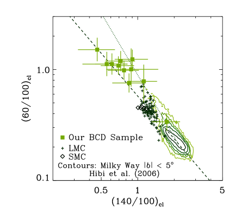
Figure 1: Far-infrared colour–colour diagram showing the relation between 60 $\mu$m–100 $\mu$m colour and 140 $\mu$m–100 $\mu$m colour. The filled squares with error bars indicate the current BCD sample, while the crosses and open diamonds show the DIRBE data of the LMC and the SMC, respectively, taken from Hibi et al. (2006). We also present the Milky Way data (with Galactic latitudes of $|b|<5^{\circ}$) adopted from Hibi et al. (2006) by the contours, which show the levels where 50, 80, 90, 95, and 99 per cent of the data are contained. The dashed line and the dotted lines present the fittings for the main correlation (equation 15) and the subcorrelation (equation 16), respectively.

It is interesting that not only the LMC and the SMC but also the current BCD sample has consistent FIR colours to the main correlation or the subcorrelation (Fig. 1). This implies that the wavelength dependence of the FIR emissivity is not different among the BCDs, the LMC, the SMC, and the Milky Way. In the following section, we examine if the FIR colours of BCDs can really be reproduced with the emission properties adopted by HHS07, who explained the FIR colours of the Milky Way, the LMC, and the SMC (Section 2).

4 Results

4.1 Interstellar radiation field

We present the dependence of FIR colours on ISRF. Here we adopt $A_{V}=0$ (i.e. the optically thin extreme for the ISRF; Section 2.3) to concentrate only on the effects of ISRF intensity. In Fig. 2, we show the FIR colour–colour relation ($(60/100)_{\mathrm{cl}}$ and $(140/100)_{\mathrm{cl}}$) calculated for silicate and graphite. We observe that the FIR colours of the BCD sample can be reproduced with $\chi\sim 30$–300 except for the lowest data point (II Zw 71). This is consistent with the conclusion in H08 that the ISRF (especially the UV ISRF, which contributes most to the dust heating) in BCDs can be 100 times higher than the Galactic ISRF in the solar neighbourhood.

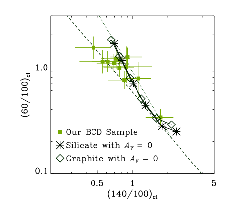
Figure 2: Far-infrared colour–colour relations for silicate and graphite (asterisks and open diamonds, respectively). The different points correspond to $\chi=1$, 3, 10, 30, 100, and 300 from high to low [140/100]. We adopt $A_{V}=0$ (optically thin extreme) for the ISRF. The same data as shown in Fig. 1 as well the the main correlation and subcorrelation (dashed and dotted lines, respectively) are also presented.

Our results not only confirm the warm IRAS (Infrared Astronomical Satellite) 60 $\mu$m–100 $\mu$m colours of BCDs (Hoffman et al., 1989), but also show high temperatures of dust contributing to the emission at $\lambda>100~{}\mu$m. A few Virgo Cluster BCDs observed by ISO (Infrared Space Observatory) show relatively cold 170 $\mu$m–100 $\mu$m colours (Popescu et al., 2002), indicating that the presence of warm dust is not necessarily the case at least in cluster environments.

We also find that the calculated FIR colours cover the area between the main correlation and the subcorrelation. With $\chi\la 10$, the colours trace the main correlation, which is appropriate for the Milky Way, the LMC and the SMC. On the other hand, the FIR colours are rather similar to the subcorrelation for $\chi\ga 100$. While Hibi et al. (2006) and HHS07 claimed that the subcorrelation can be reproduced with dust emission with multiple temperature components, we see here that the upper part of the subcorrelation can be explained with a single temperature.

4.2 Radiative transfer effects

If radiative transfer effects are considered, FIR emission comes from dust at different optical depths, where the ISRF intensities are different because of dust extinction. As modeled in Section 2.3, the FIR intensity is the sum of all contributions from different optical depths. Hibi et al. (2006) expect that radiation transfer effects shift the FIR colours toward the subcorrelation on the colour–colour diagram.

In Fig. 3, we show the FIR colours for $\chi=3$, 30, and 300 with various values of $A_{V}$ ($A_{V}=0$, 0.1, 0.2, 0.5, 1, and 2). The FIR colours change little for $A_{V}\ga 2$, since the emission is negligible from such large optical depths in the wavelength range of interest because of low dust temperatures. As expected by Hibi et al. (2006), there is a slight trend that the colours move toward the subcorrelation for $\chi\la 30$. However, we observe that the radiative transfer effects shift the FIR colours along the main correlation or the subcorrelation for $\chi\ga 30$. This indicates that the radiative transfer effects are hard to be distinguished from the change of $\chi$ on the colour–colour diagram.

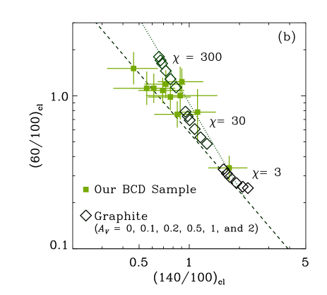
Figure 3: Far-infrared colour–colour relations for (a) silicate and (b) graphite (asterisks and open diamonds, respectively). The results for $\chi=3$, 30, and 300 are shown. For each value of $\chi$, $A_{V}=0$, 0.1, 0.2, 0.5, 1, and 2 correspond to the data points from low to high $(140/100)_{\mathrm{cl}}$. Note that $A_{V}=0$ is the optically thin extreme for the ISRF. The same data as shown in Fig. 1 as well the the main correlation and subcorrelation (dashed and dotted lines, respectively) are also presented.

How can we distinguish the variation of $A_{V}$ from that of $\chi$? We expect that if the change of $A_{V}$ controls the colour variation there may be a correlation between dust content and FIR colours. Below we further discuss the observed FIR colours in BCDs in terms of the dust content.

5 Discussion

5.1 Dust content and FIR colours

The dust mass of the current BCD sample is estimated by the WIDE-S ($90~{}\mu$m) and WIDE-L ($140~{}\mu$m) fluxes, which are suitable to trace the total mass of large grains which have the dominant contribution to the total dust content (Galliano et al., 2005). The dust mass $M_{\mathrm{d}}$ is related to the flux as (e.g. Hildebrand 1983; H08)

$$M_{\mathrm{d}}=\frac{F_{\nu}(\lambda)D^{2}}{\kappa_{\nu}B_{\nu}(T_{\mathrm{d}})}\,,$$ (17)

where $\kappa_{\nu}$ is the mass absorption coefficient of dust grains. The mass absorption coefficient is related with the absorption efficiency $Q_{\nu}$ as (e.g. H08)

$$\kappa_{\nu}=\frac{3Q_{\nu}}{4as}\,,$$ (18)

where $s$ is the grain material density. If the grain radius is much smaller than the wavelength, $Q_{\nu}/a$ is independent of $a$ (Hildebrand, 1983). The values adopted in Section 2.2 indicate $Q_{\nu}/a=1.14\times 10^{-2}~{}\mu\mathrm{m}^{-1}$ for silicate and $1.23\times 10^{-2}~{}\mu\mathrm{m}^{-1}$ for graphite at $\lambda=125~{}\mu$m. By adopting typical densities for silicate and graphite as $s=3.3$ g cm^-3 and 2.25 g cm^-3, respectively, we obtain the mass absorption coefficients at $\lambda=125~{}\mu$m as $\kappa_{125}=25.9$ and 41.0 cm² g^-1 for silicate and graphite, respectively. H08 derived $\kappa_{125}=18.8$ cm² g^-1 based on Hildebrand (1983).

Following H08, we adopt the following expression for $\kappa_{\nu}$ to estimate the dust mass from the AKARI data:

$$\kappa_{\nu}=\kappa_{125}\left(\frac{\lambda}{125~{}\mu\mathrm{m}}\right)^{-\beta}\,.$$ (19)

The absorption coefficient adopted in Section 2.2 cannot be fitted with a single power law, but the index lies between $\beta=1$ and 2. Thus, if we adopt the wavelength dependence described in Section 2.2, the estimated dust mass should be between the dust masses obtained with $\beta=1$ and $\beta=2$. We prefer to adopt this simple power-law expression for $\kappa_{\nu}$ here, since it can be directly compared with the results in H08 and the simple expression is useful for observational usage.

In Table 2, we list the dust mass estimated from equation (17). We determine the dust temperature $T_{\rm d}$ by fitting $A\nu^{\beta}B_{\nu}(T_{\rm d})$ ($A$ is a constant) to the 90 $\mu$m and 140 $\mu$m fluxes. Note that $A$ can be eliminated if we take the flux ratio of those two bands. The estimated dust temperatures are listed in Table 2, where $T_{\mathrm{d}}(\beta=1)$ and $T_{\mathrm{d}}(\beta=2)$ denote the dust temperatures evaluated with $\beta=1$ and 2, respectively. For the mass absorption coefficient, we adopt $\kappa_{125}=25.9$ cm² g^-1 (i.e. the value for silicate), but the dust mass is simply proportional to $\kappa_{125}^{-1}$ if another value of $\kappa_{125}$ is adopted. The distance is taken from H08 for the common sample, and is estimated by using the Galactocentric velocity taken from the NASA/IPAC Extragalactic Database (NED) by assuming a Hubble constant of 75 km s^-1 Mpc^-1. The dust masses estimated with $\beta=1$ and 2 are denoted as $M_{\mathrm{d}}(\beta=1)$ and $M_{\mathrm{d}}(\beta=2)$, respectively. Although the complex dependence of quantities in equation (17) makes it hard to obtain an analytical estimate of the uncertainty in $M_{\mathrm{d}}$, we have confirmed that the uncertainty is around a factor of 2 by varying the measured fluxes within the errors. From Table 2, we observe that $M_{\mathrm{d}}(\beta=1)$ is systematically smaller than $M_{\mathrm{d}}(\beta=2)$ by a factor of $\sim 2.5$, mainly because of higher dust temperature for $\beta=1$.

Table 2: Some derived and compiled quantities.

Name	$D\,^{\mathrm{a}}$	$T_{\mathrm{d}}(\beta=1)\,^{\mathrm{b}}$	$T_{\mathrm{d}}(\beta=2)\,^{\mathrm{b}}$	$M_{\mathrm{d}}(\beta=1)\,^{\mathrm{c}}$	$M_{\mathrm{d}}(\beta=2)\,^{\mathrm{c}}$	$M_{\mathrm{H\,I}}\,^{\mathrm{d}}$	$12+\log\mathrm{(O/H)}\,^{\mathrm{e}}$
	[Mpc]	[K]	[K]	[$M_{\odot}$]	[$M_{\odot}$]	[$M_{\odot}$]
UM 420	234	${97^{+249}_{-31}}$	$50^{+20}_{-9}$	$2.5\times 10^{5}$	$8.7\times 10^{5}$	—	$7.93\pm 0.05$
Mrk 59	10.9	$44^{+15}_{-7}$	$32^{+7}_{-3}$	$2.2\times 10^{4}$	$6.2\times 10^{4}$	—	$7.99\pm 0.01$
Mrk 487	11.0	$62^{+72}_{-16}$	$40^{+16}_{-7}$	$1.7\times 10^{3}$	$5.0\times 10^{3}$	$8.0\times 10^{7}$	$8.06\pm 0.04$
SBS 1319+579	29.0	$34^{+7}_{-4}$	$26^{+4}_{-2}$	$6.8\times 10^{4}$	$1.8\times 10^{5}$	$1.7\times 10^{9}$	$8.10\pm 0.01$
II Zw 40	9.2	$53^{+20}_{-9}$	$36^{+8}_{-4}$	$2.8\times 10^{4}$	$8.3\times 10^{4}$	$2.0\times 10^{8}$	$8.15\pm 0.02$
Mrk 7	42.4	$28^{+4}_{-2}$	$23^{+3}_{-1}$	$1.0\times 10^{6}$	$2.7\times 10^{6}$	$3.6\times 10^{9}$	$8.54\pm 0.04$
Mrk 71	3.4	$42^{+10}_{-5}$	$31^{+5}_{-3}$	$3.9\times 10^{3}$	$1.1\times 10^{4}$	$1.2\times 10^{9}$	$7.83\pm 0.02$
UM 439	13.1	$39^{+10}_{-5}$	$30^{+4}_{-3}$	$9.8\times 10^{3}$	$2.7\times 10^{4}$	$1.7\times 10^{8}$	$7.98\pm 0.03$
UM 533	10.9	$36^{+7}_{-5}$	$28^{+4}_{-3}$	$1.6\times 10^{4}$	$4.2\times 10^{4}$	$5.8\times 10^{7}$	$8.10\pm 0.04$
II Zw 70	17.0	$34^{+15}_{-5}$	$27^{+8}_{-4}$	$5.9\times 10^{4}$	$1.5\times 10^{5}$	$3.6\times 10^{8}$	$8.11\pm 0.04$
II Zw 71	18.5	$22^{+2}_{-2}$	$19^{+1}_{-2}$	$7.4\times 10^{5}$	$1.8\times 10^{6}$	$7.3\times 10^{8}$	$8.24\pm 0.04$

^a Distance estimated by using the Galactocentric velocity taken fro NED by assuming a Hubble constant of 75 km s^-1 Mpc^-1 except for Mrk 71, whose distance is taken from Tolstoy et al. (1995).

^b Dust temperature estimated from the 140 $\mu$m–100 $\mu$m colour (Section 5.1). The emissivity index adopted is also indicated ($\beta=1$ or 2).

^c Dust mass estimated in Section 5.1. The emissivity index adopted is also indicated ($\beta=1$ or 2).

^d H i gas mass estimated from H i 21 cm line observations. For the latter seven BCDs, the data are compiled in Hirashita et al. (2008). The data for Mrk 487 and SBS 1319+579 are obtained from Hopkins et al. (2002) and Huchtmeier et al. (2007), respectively.

^e Oxygen abundance compiled in Hopkins et al. (2002) and Hirashita et al. (2002) (and the references therein). When the error estimate is not available, we put a typical uncertainty in the measurement (0.04) (Shi et al., 2005).

As an indicator of dust abundance, we take dust-to-gas ratio. For the gas mass, we adopt H i gas mass $M_{\mathrm{H\,I}}$ estimated from H i 21 cm emission observations. The data of $M_{\mathrm{H\,I}}$ are already compiled by H08 for the common sample (i.e. the latter seven BCDs in Table 2). Among the newly added sample, there is no available H i data for UM 420 and Mrk 59, while the data for Mrk 487 and SBS 1319+579 are obtained from Hopkins, Schulte-Ladbeck, & Drozdovsky (2002) and Huchtmeier et al. (2007), respectively (for the latter, we used the formula in Lisenfeld & Ferrara 1998 to convert the H i flux to $M_{\mathrm{H\,I}}$). The dust-to-gas ratio $\mathcal{D}$ is defined as $\mathcal{D}\equiv M_{\mathrm{d}}/M_{\mathrm{H\,I}}$. We adopt $M_{\mathrm{d}}(\beta=1)$ for the dust mass, but the following discussion does not change if we adopt $M_{\mathrm{d}}(\beta=2)$.

Fig. 4 shows the relations between FIR colour ($(60/100)_{\mathrm{cl}}$ or $(140/100)_{\mathrm{cl}}$) and dust-to-gas ratio. We observe correlations with correlation coefficients $r=-0.65$ for the $\log(60/100)_{\mathrm{cl}}$–$\log\mathcal{D}$ relation and $r=0.89$ for the $\log(140/100)_{\mathrm{cl}}$–$\log\mathcal{D}$ relation. These correlations indicate that the dust temperature tends to be high in dust-poor objects. We present not only the sample BCDs but also the data of the Milky Way, the LMC and the SMC. The dust-to-gas ratio of the Milky Way is assumed to be 0.006 (Spitzer, 1978), while the dust-to-gas ratios of the LMC and the SMC are assumed to be 1/3 and 1/5 times of the value of the Milky Way (Pei, 1992). For the FIR colours, we adopt the peak of the contours in Fig. 1 for the Milky Way, and the average of the data points for the LMC and the SMC. Those three points also follow the trend found by the BCDs.

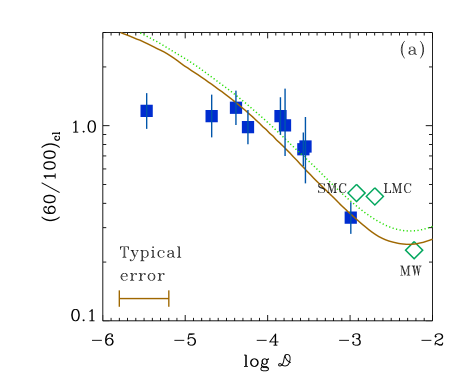
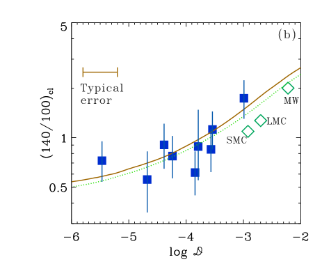
Figure 4: Relation between far-infrared colour ($(60/100)_{\mathrm{cl}}$ and $(100/140)_{\mathrm{cl}}$ in Panels a and b, respectively) and dust-to-gas ratio. The filled squares with vertical error bars represent the current BCD sample whose H i mass is available. The typical error of dust-to-gas ratio which comes from the error of estimated dust mass is shown by the horizontal bar. The data points for the Milky Way, the LMC and the SMC are also presented by the open diamonds. The solid and dotted lines show the colour variation expected from the model described by equation (21) with the optically thin extreme ($A_{V}=0$) for silicate and graphite, respectively. The correlation coefficients for the BCD data are $r=-0.65$ and $r=0.89$ for Panels a and b, respectively.

A possible interpretation of the correlation in Fig. 4 is that the relatively low dust temperatures in dust-rich BCDs result from the shielding (extinction) of stellar radiation. In order to examine this possibility, we calculate the relation between FIR colours and $A_{V}$ by using the models (same as Fig. 3). The results are shown in Fig. 5, where we find that both the variation of $(60/100)_{\mathrm{cl}}$ and that of $(140/100)_{\mathrm{cl}}$ with a single value of $\chi$ are too small to explain the observed large diversity in these colours in Fig. 4. The colours are not so sensitive to the change of $A_{V}$ partly because the strongest contribution from $A_{V}\sim 0$, where the dust temperature is the highest, is always present. In particular, if $A_{V}\ga 2$, the colour is insensitive to $A_{V}$ since the dust temperature at such deep optical depths is too low to contribute to the total emission. Thus, the variation of the FIR colours cannot be reproduced only with a variation of dust optical depth, but rather it should reflect the correlation (i) between dust-to-gas ratio and dust heating itself (i.e., ISRF), or (ii) between dust-to-gas ratio and dust properties (i.e., absorption coefficient and/or grain size distribution).

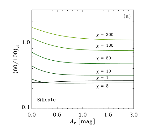
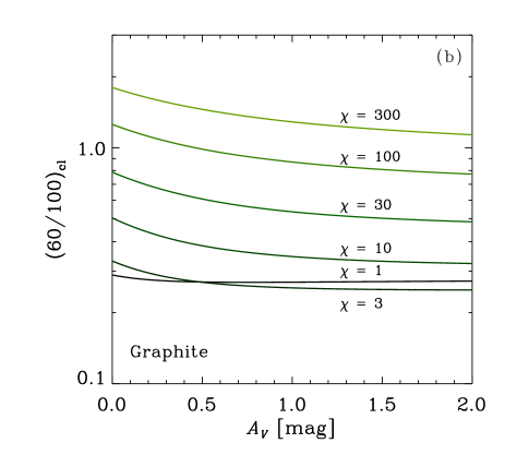
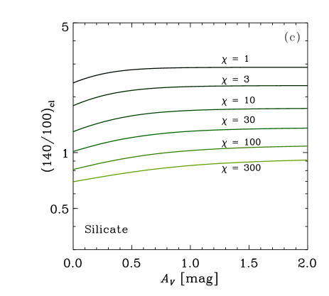
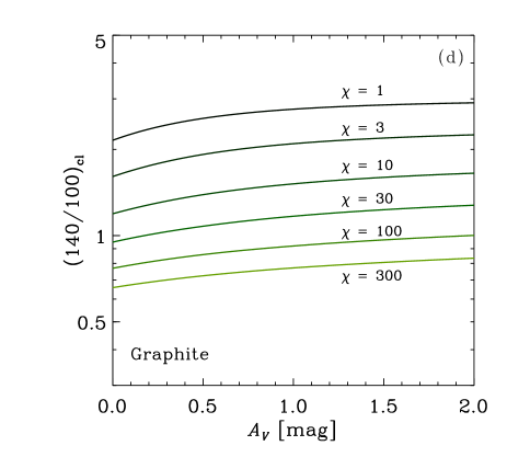
Figure 5: Far-infrared colours ($(60/100)_{\mathrm{cl}}$ in Panels a and b, and $(100/140)_{\mathrm{cl}}$ in Panels c and d) for a foreground screen as a function of $A_{V}$. For the grain species we examine silicate (Panels a and c) and graphite (Panels b and d). In each panel, different lines show different ISRF intensities of $\chi=1$, 3, 10, 30, 100, and 300.

It is difficult to survey all the possible cases for (ii), since there are few, if any, constraints on the dust properties in BCDs. However, we can discuss some cases for (ii) as follows. HHS07 show that $(140/100)_{\mathrm{cl}}$ changes only slightly along with the change of grain size distribution, since it reflects the equilibrium grain temperature. Thus, it is hard to reproduce the clear correlation between $(140/100)_{\mathrm{cl}}$ and dust-to-gas ratio only with the change of grain size distribution. The change of grain material as a function of dust-to-gas ratio may change the grain absorption coefficient, leading to variation of dust temperature as a function of dust-to-gas ratio. However, we have shown that the colour–colour relation of the BCDs can be explained by the emissivity that also explains the colour–colour relation of the Milky Way. In this context, it is not probable that the dust property is the main driver for the change of FIR colours.

The possibility (i) is interesting to investigate, since the correlation in Fig. 4 is a natural extension of the sequence of the Milky Way, the LMC, and the SMC. For those “nearby” three galaxies, it is known that the typical ISRFs are different (e.g. Welty et al., 2006), and indeed the FIR colour sequence can be explained by the variation of the ISRF (Hibi et al. 2006, HHS07). Thus, in the following subsection, we discuss a possibility that the ISRF changes as a function of dust-to-gas ratio.

5.2 Correlation between dust-to-gas ratio and ISRF?

Here we interpret the correlation between dust-to-gas ratio and FIR colours as the correlation between dust-to-gas ratio and ISRF. Since the main heating source of dust grains is UV photons coming from the young stellar population (Buat & Xu, 1996), the dust-heating ISRF reflects the spatial concentration of recent star formation activity. Thus, the correlation between dust-to-gas ratio and ISRF indicates that dust-poor galaxies tend to host concentrated star-forming regions.

There are some theoretical models which suggest that dust plays an active role in determining the properties of star formation. Indeed Hirashita & Hunt (2004) show that the shielding of UV heating photons plays an important role in determining the strength of star formation: If the optical depth of dust becomes large, the UV heating photons are efficiently blocked and the gas efficiently cools to produce a favourable condition for the star formation. Thus, the optical depth of dust in UV is important, and a burst of star formation could become possible if the UV optical depth exceeds one. In this scenario, the condition for star formation can be written as

$$\kappa\mathcal{D}\rho R\sim 1\,,$$ (20)

where $\kappa$ is the UV absorption coefficient per dust mass and $R$ is the size of the star-forming region. On the other hand, we assume that a constant fraction of gas mass is converted to stars: $L\propto M_{\mathrm{gas}}$, where $M_{\mathrm{gas}}(\sim\rho R^{3})$ is the gas mass, and $L$ is the stellar UV luminosity. Since $\chi\propto L/R^{2}\propto M_{\mathrm{gas}}/R^{2}\sim\rho R$, we obtain $\chi\propto\mathcal{D}^{-1}$ by using equation (20). Normalizing the quantities to the Milky Way values (i.e. $\chi=1$ and $\mathcal{D}=0.006$), we obtain

$$\chi=\left(\frac{\mathcal{D}}{0.006}\right)^{-1}\,.$$ (21)

In Fig. 4, we calculate the relation between the FIR colours and $\mathcal{D}$ by assuming equation (21). The optically thin extreme (i.e. $A_{V}=0$) for the ISRF is adopted to focus on the effect of $\chi$. The results indeed traces the trend of the observational data. Thus, the above argument on dust shielding of UV photons (equation 20) as the condition for a burst of star formation is compatible with the data.

Equation (20) implies that the size-density relation of star-forming region becomes roughly a relation with constant column density. Indeed, the observational data presented by Hirashita & Hunt (2009) support constant column density of star-forming regions in BCDs (i.e. $\rho\propto R^{-1}$). Pak et al. (1998) also find that the column density of gas is inversely proportional to the dust-to-gas ratio based on an analysis of photodissociation regions in the Milky Way, the LMC, and the SMC, which is consistent with our picture. McKee (1989) show that an equilibrium between the gravitational contraction and the energy injection from stars is achieved at $A_{V}\sim 4$–8 based on the stability argument on photoionization-regulated star formation, in which shielding of photoionizing photons permits ambipolar diffusion to proceed and stars to form. Although the physical processes considered in McKee (1989) are more detailed and sophisticated, the necessity of shielding is common with our picture expressed in equation (20).

5.3 FIR colour and metallicity

The observational correlation between FIR colour and dust-to-gas ratio shown in this paper has confirmed the results of Engelbracht et al. (2008), who show the correlation between Spitzer MIPS 70 $\mu$m–160 $\mu$m colour and metallicity. Since there is a correlation between dust-to-gas ratio and metallicity as shown by them and also by H08, the correlation with metallicity is equivalent to the correlation with dust-to-gas ratio. For the detailed discussions on the relation between dust-to-gas ratio and metallicity in BCDs, see H08 and Lisenfeld & Ferrara (1998).

Fig. 6 shows the relation between FIR colour and metallicity (oxygen abundance in gas phase) for the BCD sample. The data of oxygen abundance are compiled in Hirashita, Tajiri, & Kamaya (2002) and Hopkins et al. (2002), and summarized in Table 2. We observe correlations with $r=-0.45$ for the relation between $\log(60/100)_{\mathrm{cl}}$ and $12+\log(\mathrm{O/H})$ and $r=0.53$ for the relation between $\log(140/100)_{\mathrm{cl}}$ and $12+\log(\mathrm{O/H})$. We also show the data points for the Milky Way, the LMC, and the SMC. The Milky Way gas metallicity is represented by the Orion Nebula ($12+\log(\mathrm{O/H})=8.58$), which has a similar metallicity to local B-type stars (Peimbert, 1987; Gies & Lambert, 1992; Kilian, 1992; Mathis, 2000). For the LMC and the SMC, we adopt the oxygen abundance from Dufour (1984) ($12+\log(\mathrm{O/H})=8.43$ and 8.02, respectively). We confirm that metal-poor galaxies tend to have high dust temperatures.

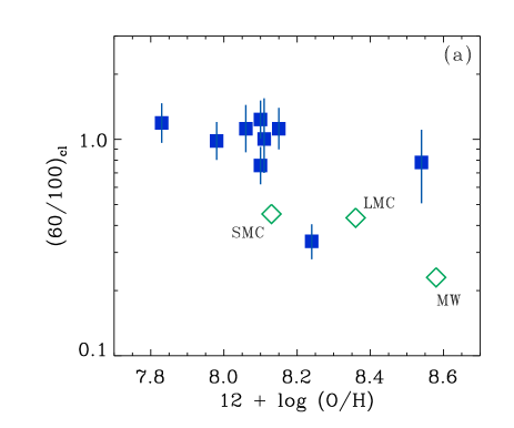
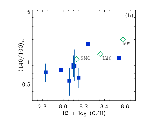
Figure 6: Relation between FIR colour ($(60/100)_{\mathrm{cl}}$ and $(100/140)_{\mathrm{cl}}$ for Panels a and b, respectively) and oxygen abundance. The filled squares with vertical error bars represent the same BCD sample as in Fig. 4. The data points for the Milky Way, the LMC and the SMC are also presented by the open diamonds. The uncertainty in the oxygen abundance measurement is shown in Table 2. The correlation coefficients for the BCD data are $r=-0.45$ and $r=0.53$ for Panels a and b, respectively.

We should keep in mind that the story of star formation properties in terms of metallicity is not so simple as we discussed above. Engelbracht et al. (2008) show that the dust temperature shows the peak around $12+\log(\mathrm{O/H})\sim 8$. Due to our small sample in such a low metallicity range, we cannot confirm it, but their results imply that the size and density of star-forming region is not a monotonic function of metallicity. There are also pieces of evidence that there are two categories of BCDs: “active” and “passive”. The former hosts compact and intense star formation activities, while the latter has diffuse star formation properties (Hunt, Giovanardi, & Helou, 2002; Hirashita & Hunt, 2004). Even with a similar metallicity, such a dichotomy exists, indicating that the star formation properties are not determined simply by the metallicity. Active BCDs tend to be luminous in FIR because of large dust optical depth (Hirashita & Hunt, 2004). Thus, it would be possible that the current sample is biased to the “active” class. The presence of BCDs hosting cold dust in Virgo Cluster (Popescu et al., 2002) also implies that such a bias could be present. This kind of bias should be examined in the future with more sensitive facilities.

Finally, it is worth questioning which of dust-to-gas ratio and metallicity is more fundamental in regulating dust temperature. Larger absolute values of correlation coefficient found in Fig. 4 than those in Fig. 6 imply that dust-to-gas ratio rather than metallicity is more strongly connected with dust temperature. Thus, we here suggest that dust-to-gas ratio is more fundamental than metallicity in regulating the dust temperature. This should be further examined with a larger sample.

5.4 Importance of submillimetre data

It is expected that the radiative transfer effect, i.e. the shielding effect of dust can be seen more clearly in submillimetre (submm) than in FIR, since the submm emission can trace dust with lower temperature (e.g. Galliano et al., 2003). Although the submm data of the current BCD sample are still lacking except for those of II Zw 40, future more sensitive submm facilities such as Herschel and ALMA will increase the data.

We adopt $\lambda=850~{}\mu$m as a representative submm wavelength, and examine the relation between $(850/100)_{\mathrm{cl}}$ and $(60/100)_{\mathrm{cl}}$; that is, we adopt $\lambda=850~{}\mu$m instead of $\lambda=140~{}\mu$m, which is adopted in the rest of this paper. In Fig. 7, we present the colour–colour relation with $A_{V}=0$ (i.e. without the radiative transfer effect; Section 2.3). We also show the nearby galaxy sample observed at $\lambda=850~{}\mu$m by Dunne et al. (2000), who also list the IRAS 60 $\mu$m and 100 $\mu$m fluxes. We observe that the prediction traces the trend of the data, indicating that the submm flux is naturally explained by the natural extension of the FIR SED. This means that a very cold component contributing only to the submm flux is not necessary for a major part of the nearby galaxies.

Galliano et al. (2003, 2005) argue that a very cold component should be introduced for metal-poor dwarf galaxies. In particular, II Zw 40, which is included also in the current sample, shows a clear excess of the submm flux. In Fig. 7, we also plot the data point taken from Galliano et al. (2005) for II Zw 40 (see also Hunt, Bianchi, & Maiolino 2005). Indeed, we observe a clear deviation from the model prediction, which can be interpreted as a significant contribution from a very cold component. They also propose that such very cold dust should be located in an environment where the stellar radiation is strongly shielded. In order to examine the effect of shielding (i.e. radiative transfer), we show the results with $A_{V}>0$ in Fig. 8. We observe that $(850/100)_{\mathrm{cl}}$ increases even for $A_{V}>2$ while $(60/100)_{\mathrm{cl}}$ is almost constant for such large $A_{V}$. This confirms that 850 $\mu$m flux is also sensitive to the shielded cold dust grains. Fig. 8 also demonstrates that the data point of II Zw 40 is explained with $A_{V}\sim 5$ with $\chi\sim 300$. Thus we conclude the existence of shielded cold dust in II Zw 40 (and in other galaxies whose data points deviate rightwards in Fig. 7). Galliano et al. (2005) also show that the UV ISRF of II Zw 40 is higher than that of the Milky Way by two orders of magnitude.

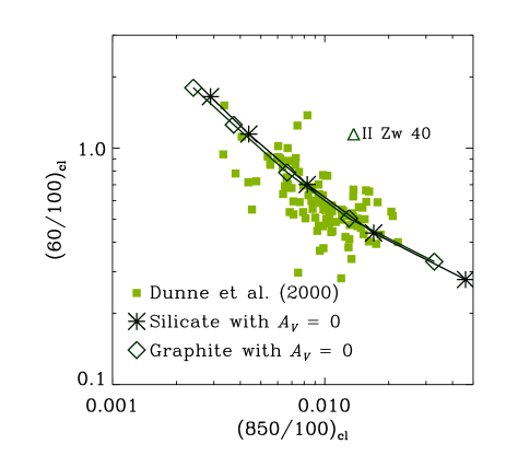
Figure 7: $(60/100)_{\mathrm{cl}}$–$(850/100)_{\mathrm{cl}}$ relations for silicate and graphite (asterisks and open diamonds, respectively). The different points correspond to $\chi=3$, 10, 30, 100, and 300 from high to low $(850/100)_{\mathrm{cl}}$. The optically thin extreme for the ISRF ($A_{V}=0$) is adopted. The filled squares indicate the observational data of nearby galaxies in Dunne et al. (2000) and the open triangle shows the data point of II Zw 40 taken from Galliano et al. (2005).

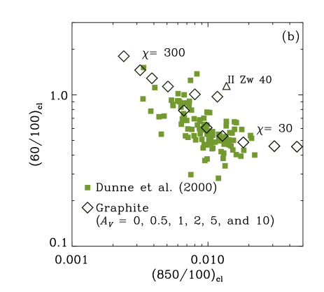
Figure 8: $(60/100)_{\mathrm{cl}}$–$(850/100)_{\mathrm{cl}}$ relations for (a) silicate and (b) graphite (asterisks and open diamonds, respectively). The results with $\chi=30$ and 300 are shown. For each value of $\chi$, $A_{V}=0$, 0.5, 1, 2, 5, and 10 correspond to the data points from low to high $(850/100)_{\mathrm{cl}}$ (the point for $\chi=30$ and $A_{V}=10$ is out of the range). Note that $A_{V}=0$ is the optically thin extreme for the ISRF. The nearby galaxy data taken from Dunne et al. (2000) are presented by the filled squares.

Although our interpretation of the submm excess as a contribution from the shielded cold dust component is in agreement with the analysis by Galliano et al. (2005), there is quantitative difference between our results and theirs. Galliano et al. (2005) adopted $Q_{\mathrm{abs}}\propto\lambda^{-2}$ at $\lambda>100~{}\mu$m. If the absorption efficiency is normalized to the value at $\lambda=100~{}\mu$m, the absorption efficiency adopted in this paper (equation 11) is 2 times larger than that used in Galliano et al. (2005) at $\lambda=850~{}\mu$m. Therefore, we require less very cold dust component than Galliano et al. (2005) by a factor of 2.

5.5 Common dust optical properties?

In this paper, we have adopted a common FIR dust optical properties; that is, we have applied the same absorption efficiency $Q_{\mathrm{abs}}$ and grain size distribution as adopted in our previous model for the Milky Way and the Magellanic Clouds (HHS07). The same dust optical properties are also consistent with the FIR colours of BCDs. Hibi et al. (2006) and HHS07 also argue that those dust optical properties also provide a good statistical fit to the FIR colours of nearby galaxies. Therefore, we suggest that the absorption efficiency in the form of equation (11), which Reach et al. (1995) adopted to fit the dust emission spectra in the Milky Way, is generally applicable in galactic environments. As shown above, the submm emission from nearby galaxies can also be explained by the same dust emissivity.

It is also important to stress that the classical dust emissivity model by Draine & Lee (1984) cannot explain the FIR colour–colour relation of the nearby galaxies (Hibi et al. 2006; HHS07). As indicated by the emissivity assumed by Reach et al. (1995), it is better to adopt $\beta\sim 1$ for $100~{}\mu\mathrm{m}\la\lambda\la\lambda_{1}\sim 200~{}\mu$m rather than to assume $\beta\sim 2$ in the entire FIR wavelength range longer than 100 $\mu$m. Some amorphous materials indeed show $\beta<2$ (e.g. Agladze et al., 1996). Amorphous grains are expected to form by the irradiation of cosmic rays (Jäger et al., 2003).

Theoretically the break of the dust emissivity at $\lambda_{1}$ might be associated with the energy splitting of the ground state because of irregular amorphous structure. Meny et al. (2007) show that the absorption coefficient of amorphous dust has a break at $\lambda\sim\lambda_{\mathrm{m}}$, which corresponds to the cut-off energy $\hbar\omega_{\mathrm{m}}$ of the energy splitting due to the amorphous structure ($\omega_{\mathrm{m}}\equiv 2\pi c/\lambda_{\mathrm{m}}$). Therefore, a possible interpretation is that $\lambda_{\mathrm{m}}\sim\lambda_{1}$. Since Meny et al. (2007) suggest $\lambda_{\mathrm{m}}\sim 700~{}\mu$m based on experimental data, the cut-off energy corresponding to $\lambda_{\mathrm{m}}\sim 200~{}\mu$m may be too high. Nevertheless it is still worth investigating amorphous materials with higher cut-off energy as a candidate of cosmic dust.

6 Conclusion

We have investigated the properties of FIR emission of a sample of BCDs observed by AKARI, especially focusing on FIR colours and dust temperature. We have utilized the data at $\lambda=65~{}\mu$m, 90 $\mu$m, and 140 $\mu$m, and have examined the relation between 60 $\mu$m–100 $\mu$m colour, $(60/100)_{\mathrm{cl}}$, and 140 $\mu$m–100 $\mu$m colour $(140/100)_{\mathrm{cl}}$. Then, we have found that the FIR colours of the BCDs are located at a natural high-temperature extension of the DIRBE data of the Milky Way, the LMC and the SMC on the colour–colour diagram. We have explained the FIR colours also theoretically by assuming the same absorption efficiency, which may be appropriate for amorphous dust grains, and the same grain size distribution as the Milky Way dust. We have also shown that it is not easy to distinguish between a large dust optical depth and a low dust temperature only with FIR colours although addition of submillimetre data relax this degeneracy.

In order to examine if the dust optical depth plays an important role in determining the dust temperature, we have investigated the correlation between FIR colour (dust temperature) and dust-to-gas ratio. We have found that the dust temperature tends to become high as the dust-to-gas ratio decreases as would be expected from the shielding effect of stellar radiation by dust. However, we fail to explain this trend quantitatively only by the effect of dust optical depth. Thus, we conclude that there is a relation between dust-to-gas ratio and interstellar radiation field (ISRF) intensity. This relation is consistent with a “constant dust optical depth” of star-forming regions in BCDs, implying that dust extinction plays an important role in determining the condition for a burst of star formation.

The correlation between dust-to-gas ratio and dust temperature is equivalent to that between metallicity and dust temperature found in Engelbracht et al. (2008), since there is a correlation between dust-to-gas ratio and metallicity. By comparing the correlation strengths, we propose that dust-to-gas ratio is more fundamental than metallicity in regulating dust temperature, although we will have to confirm this with a larger sample.

References

- Agladze et al. (1996) Agladze, N. I., Sievers, A. J., Jones, S. A., Burlitch, J. M., & Beckwith, S. V. W. 1996, ApJ, 462, 1026
- Bianchi, Davies, & Alton (1999) Bianchi, S., Davies, J. I., & Alton, P. B. 1999, A&A, 344, L1
- Bohren & Huffman (1983) Bohren, C. F., & Huffman, D. R. 1983, Absorption and Scattering of Light by Small Particles, Wiley, New York
- Boselli et al. (2003) Boselli, A., Gavazzi, G., & Sanvito, G. 2003, A&A, 402, 37
- Buat & Xu (1996) Buat, V., & Xu, C. 1996, A&A, 306, 61
- (6) Cardelli, J. A., Clayton, G. C., & Mathis, J. S. 1989, ApJ, 345, 245
- Désert, Boulanger, & Puget (1990) Désert, F.-X., Boulanger, F., & Puget, J. L. 1990, A&A, 237, 215
- Dopita et al. (2005) Dopita, M. A., et al. 2005, ApJ, 619, 755
- Draine & Lee (1984) Draine, B. T., & Lee, H. M. 1984, ApJ, 285, 89
- Draine & Li (2001) Draine, B. T., & Li, A. 2001, ApJ, 551, 807
- Dufour (1984) Dufour, R. J. 1984, in Structure and Evolution of the Magellanic Clouds, ed. S. van den Bergh, & K. S. de Boer (Kluwer, Dordrecht), p. 353
- Dunne et al. (2000) Dunne, L., Eales, S., Edmunds, M., Ivison, R., Alexander, P., Clements, D. L. 2000, MNRAS, 315, 115
- Dwek et al. (1997) Dwek, E., et al. 1997, ApJ, 475, 565
- Engelbracht et al. (2008) Engelbracht, C. W., Rieke, G. H., Gordon, K. D., Smith, J.-D. T., Werner, M. W., Moustakas, J., Willmer, C. N. A., & Vanzi, L. 2008, ApJ, 678, 804
- Galliano et al. (2005) Galliano, F., Madden, S. C., Jones, A. P., Wilson, C. D., & Bernard, J.-P. 2007, A&A, 434, 867
- Galliano et al. (2003) Galliano, F., Madden, S. C., Jones, A. P., Wilson, C. D., Bernard, J.-P., & Le Peintre, F. 2003, A&A, 407, 159
- Gies & Lambert (1992) Gies, D. R., & Lambert, D. L. 1992, ApJ, 387, 673
- Hibi (2006) Hibi, Y. 2006, PhD Thesis, Nagoya University
- Hibi et al. (2006) Hibi, Y., Shibai, H., Kawada, M., Ootsubo, T., & Hirashita, H. 2006, PASJ, 58, 509
- Hildebrand (1983) Hildebrand, R. H. 1983, QJRAS, 24, 267
- Hirashita et al. (2002) Hirashita, H., Tajiri, Y. Y., & Kamaya, H. 2002, A&A, 388, 439
- Hirashita et al. (2007) Hirashita, H., Hibi, Y., & Shibai, H. 2007, MNRAS, 379, 974 (HHS07)
- Hirashita & Hunt (2004) Hirashita, H., & Hunt, L. K. 2004, A&A, 460, 67
- Hirashita & Hunt (2009) Hirashita, H., & Hunt, L. K. 2009, A&A, submitted
- Hirashita et al. (2008) Hirashita, H., Kaneda, H., Onaka, T., & Suzuki, T. 2008, PASJ, 60, S477 (H08)
- Hoffman et al. (1989) Hoffman, G. L., Helou, G., Salpeter, E. E., & Lewis, B. M. 1989, ApJ, 339, 812
- Hopkins et al. (2002) Hopkins, A. M., Schulte-Ladbeck, R. E., & Drozdovsky, I. O. 2002, AJ, 124, 862
- Huchtmeier et al. (2007) Huchtmeier, W. K., Petrosian, A., Gopal-Krishna, Kunth, D. 2007, A&A, 462, 919
- Hunt, Giovanardi, & Helou (2002) Hunt, L. K., Giovanardi, C., & Helou, G. 2002, A&A, 394, 873
- Hunt, Bianchi, & Maiolino (2005) Hunt, L. K., Bianchi, S., & Maiolino, R. 2005, A&A, 434, 849
- Iglesias-Páramo et al. (2004) Iglesias-Páramo, J., Buat, V., Donas, J., Boselli, A., & Milliard, B. 2004, A&A, 419, 109
- Inoue et al. (2000) Inoue, A. K., Hirashita, H., & Kamaya, H. 2000, PASJ, 52, 539
- Jäger et al. (2003) Jäger, C., Fabian, D., Schrempel, F., Dorschner, J., Henning, Th., & Wesch, W. 2003, A&A, 401, 57
- Kawada et al. (2007) Kawada, M., et al. 2007, PASJ, 59, S389
- Kennicutt (1998) Kennicutt, R. C., Jr. 1998, ARA&A, 36, 189
- Kilian (1992) Kilian, J. 1992, A&A, 262, 171
- Li & Draine (2001) Li, A., & Draine, B. T. 2001, ApJ, 554, 778
- Lisenfeld & Ferrara (1998) Lisenfeld, U., & Ferrara, A. 1998, ApJ, 496, 145
- Madden et al. (2006) Madden, S. C., Galliano, F., Jones, A. P., & Sauvage, M. 2006, A&A, 446, 877
- Maiolino et al. (2004) Maiolino, R., Schneider, R., Oliva, E., Bianchi, S., Ferrara, A., Mannucci, F., Pedani, M., Roca Sogorb, M. 2004, Nature, 431, 533
- Mathis (2000) Mathis, J. S. 2000, in Allen’s Astrophysical Quantities, Fourth Edition, ed. A. N. Cox, (Springer, New York), p. 523
- Mathis et al. (1983) Mathis, J. S., Mezger, P. G., & Panagia, N. 1983, A&A, 128, 212
- Mathis, Rumpl, Nordsieck (1977) Mathis, J. S., Rumpl, W., & Nordsieck, K. H. 1977, ApJ, 217, 425
- McKee (1989) McKee, C. F. 1989, ApJ, 345, 782
- Meny et al. (2007) Meny, C., Gromov, V., Boudet, N., Bernard, J.-Ph., Paradis, D., & Nayral, C. 2007, A&A, 468, 171
- Murakami et al. (2007) Murakami, H., et al. 2007, PASJ, 59, S369
- Nagata et al. (2002) Nagata, H., Shibai, H., Takeuchi, T. T., & Onaka, T. 2002, PASJ, 54, 695
- Nozawa et al. (2003) Nozawa, T., Kozasa, T., Umeda, H., Maeda, K., & Nomoto, K. 2003, ApJ, 598, 785
- Onaka et al. (2007) Onaka, T., Tokura, D., Sakon, I., Tajiri, Y. Y., Takagi, T., & Shibai, H. 2007, ApJ, 654, 844
- Pak et al. (1998) Pak, S., Jaffe, D. T., van Dishoeck, E. F., Johansson, L. E. B., & Booth, R. S. 1998, ApJ, 498, 735
- Pei (1992) Pei, Y. C., 1992, ApJ, 395, 130
- Peimbert (1987) Peimbert, M. 1987, in Star Forming Regions, ed. M. Peimbert & J. Jugaku (Reidel, Dordrecht), p. 111
- Popescu et al. (2002) Popescu, C. C., Tuffs, R. J., Völk, H. J., Pierini, D., & Madore, B. F. 2002, ApJ, 567, 221
- Reach et al. (1995) Reach, W. T., et al. 1995, ApJ, 451, 188
- Sakon et al. (2004) Sakon, I., Onaka, T., Ishihara, D., Ootsubo, T., Yamamura, I., Tanabé, & Roellig, T. L. 2004, ApJ, 609, 203
- Sargent & Searle (1970) Sargent, W. L. W., & Searle, L. 1970, ApJ, 162, L155
- Schneider, Ferrara, & Salvaterra (2004) Schneider, R., Ferrara, A., & Salvaterra, R. 2004, MNRAS, 351, 1379
- Shi et al. (2005) Shi, F., Kong, X., Li, C., & Cheng, F. Z. 2005, A&A, 437, 849
- Spitzer (1978) Spitzer, L., Jr 1978, Physical Processes in the Interstellar Medium, New York, Wiley
- (60) Takagi, T., Vansevičius, V., & Arimoto, N. 2003, PASJ, 55, 385
- Takeuchi et al. (2005) Takeuchi, T. T., Ishii, T. T., Nozawa, T., Kozasa, T., & Hirashita, H. 2005, MNRAS, 362, 592
- Thuan, Sauvage, & Madden (1999) Thuan, T. X., Sauvage, M., & Madden, S. 1999, ApJ, 516, 783
- Todini & Ferrara (2001) Todini, P., & Ferrara, A. 2001, MNRAS, 325, 726
- Tolstoy et al. (1995) Tolstoy, E., Saha, A., Hoessel, J. G., & McQuade, K. 1995, AJ, 110, 1640
- van Zee, Skillman, & Salzer (1998) van Zee, L., Skillman, E. D., & Salzer, J. J. 1998, AJ, 116, 1186
- Verdugo et al. (2007) Verdugo, E., Yamamura, I., & Pearson, C. P. 2007, AKARI FIS Data User Manual Version 1.3
- Weingartner & Draine (2001) Weingartner, J. C., & Draine, B. T. 2001, ApJ, 548, 296
- Welty et al. (2006) Welty, D. E., Federman, S. R., Gredel, R., Thorburn, J. A., & Lambert, D. L. 2006, ApJS, 165, 138