Hessian and concavity of mutual information, differential entropy, and entropy power in linear vector Gaussian channels

Abstract

Within the framework of linear vector Gaussian channels with arbitrary signaling, closed-form expressions for the Jacobian of the minimum mean square error and Fisher information matrices with respect to arbitrary parameters of the system are calculated in this paper. Capitalizing on prior research where the minimum mean square error and Fisher information matrices were linked to information-theoretic quantities through differentiation, closed-form expressions for the Hessian of the mutual information and the differential entropy are derived. These expressions are then used to assess the concavity properties of mutual information and differential entropy under different channel conditions and also to derive a multivariate version of the entropy power inequality due to Costa.

I Introduction and motivation

Closed-form expressions for the Hessian matrix of the mutual information with respect to arbitrary parameters of the system are useful from a theoretical perspective but also from a practical standpoint. In system design, if the mutual information is to be optimized through a gradient algorithm as in [1], the Hessian matrix may be used alongside the gradient in the Newton’s method to speed up the convergence of the algorithm. Additionally, from a system analysis perspective, the Hessian matrix can also complement the gradient in studying the sensitivity of the mutual information to variations of the system parameters and, more importantly, in the cases where the mutual information is concave with respect to the system design parameters, it can also be used to guarantee the global optimality of a given design.

In this sense and within the framework of linear vector Gaussian channels with arbitrary signaling, the purpose of this work is twofold. First, we find closed-form expressions for the Hessian matrix of the mutual information, differential entropy and entropy power with respect to arbitrary parameters of the system and, second, we study the concavity properties of these quantities. Both goals are intimately related since concavity can be assessed through the negative definiteness of the Hessian matrix. As intermediate results of our study, we derive closed-form expressions for the Jacobian of the minimum mean-square error (MMSE) and Fisher information matrices, which are interesting results in their own right and contribute to the exploration of the fundamental links between information theory and estimation theory.

Initial connections between information- and estimation-theoretic quantities for linear channels with additive Gaussian noise date back from the late fifties: in the proof of Shannon’s entropy power inequality [2], Stam used the fact that the derivative of the output differential entropy with respect to the added noise power is equal to the Fisher information of the channel output and attributed this identity to De Bruijn. More than a decade later, the links between both worlds strengthened when Duncan [3] and Kadota, Zakai, and Ziv [4] independently represented mutual information as a function of the error in causal filtering.

Much more recently, in [5], Guo, Shamai, and Verdú fruitfully explored further these connections and, as their main result, proved that the derivative of the mutual information (and differential entropy) with respect to the signal-to-noise ratio (SNR) is equal to half the MMSE regardless of the input statistics. The main result in [5] was generalized to the abstract Wiener space by Zakai in [6] and by Palomar and Verdú in two different directions: in [1] they calculated the partial derivatives of the mutual information and differential entropy with respect to arbitrary parameters of the system, rather than with respect to the SNR alone, and in [7] they represented the derivative of mutual information as a function of the conditional marginal input given the output for channels where the noise is not constrained to be Gaussian.

In this paper we build upon the setting of [1], where loosely speaking, it was proved that, for the linear vector Gaussian channel

$$\boldsymbol{Y}=\mathbf{G}\boldsymbol{S}+\mathbf{C}\boldsymbol{N},$$ (1)

i) the gradients of the differential entropy $h(\boldsymbol{Y})$ and the mutual information $I(\boldsymbol{S};\boldsymbol{Y})$ with respect to functions of the linear transformation undergone by the input, $\mathbf{G}$, are linear functions of the MMSE matrix $\mathbf{E}_{\boldsymbol{S}}$ and ii) the gradient of the differential entropy $h(\boldsymbol{Y})$ with respect to the linear transformation undergone by the noise, $\mathbf{C}$, are linear functions of the Fisher information matrix, $\mathbf{J}_{\boldsymbol{Y}}$.

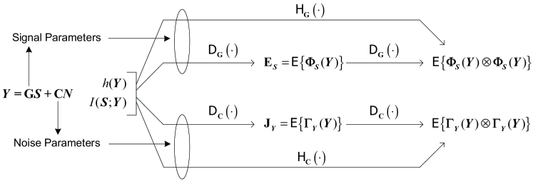
Figure 1: Simplified representation of the relations between the quantities dealt with in this work. The Jacobian, ${{\sf D}}$, and Hessian, ${{\sf H}}$, operators represent first and second order differentiation, respectively.

In this work, we show that the previous two key quantities $\mathbf{E}_{\boldsymbol{S}}$ and $\mathbf{J}_{\boldsymbol{Y}}$, which completely characterize the first-order derivatives, are not enough to describe the second-order derivatives. For that purpose, we introduce the more refined conditional MMSE matrix $\boldsymbol{\Phi}_{\boldsymbol{S}}(\boldsymbol{y})$ and conditional Fisher information matrix $\boldsymbol{\Gamma}_{\boldsymbol{Y}}(\boldsymbol{y})$ (note that when these quantities are averaged with respect to the distribution of the output $\boldsymbol{y}$, we recover $\mathbf{E}_{\boldsymbol{S}}={\sf E}\left\{\boldsymbol{\Phi}_{\boldsymbol{S}}(\boldsymbol{Y})\right\}$ and $\mathbf{J}_{\boldsymbol{Y}}={\sf E}\left\{\boldsymbol{\Gamma}_{\boldsymbol{Y}}(\boldsymbol{Y})\right\}$). In particular, the second-order derivatives depend on $\boldsymbol{\Phi}_{\boldsymbol{S}}(\boldsymbol{y})$ and $\boldsymbol{\Gamma}_{\boldsymbol{Y}}(\boldsymbol{y})$ through the following terms: ${\sf E}\left\{\boldsymbol{\Phi}_{\boldsymbol{S}}(\boldsymbol{Y})\otimes\boldsymbol{\Phi}_{\boldsymbol{S}}(\boldsymbol{Y})\right\}$ and ${\sf E}\left\{\boldsymbol{\Gamma}_{\boldsymbol{Y}}(\boldsymbol{Y})\otimes\boldsymbol{\Gamma}_{\boldsymbol{Y}}(\boldsymbol{Y})\right\}$. See Fig. 1 for a schematic representation of these relations.

Analogous results to some of the expressions presented in this paper particularized to the scalar Gaussian channel were simultaneously derived in [8, 9], where the second and third derivatives of the mutual information with respect to the SNR were calculated.

As an application of the obtained expressions, we show concavity properties of the mutual information and the differential entropy, derive a multivariate generalization of the entropy power inequality (EPI) due to Costa in [10]. Our multivariate EPI has already found an application in [11] to derive outer bounds on the capacity region in multiuser channels with feedback.

This paper is organized as follows. In Section II, the model for the linear vector Gaussian channel is given and the differential entropy, mutual information, minimum mean-square error, and Fisher information quantities as well as the relationships among them are introduced. The main results of the paper are given in Section III where we present the expressions for the Jacobian matrix of the MMSE and Fisher information and also for the Hessian matrix of the mutual information and differential entropy. In Section IV the concavity properties of the mutual information are studied and in Section V a multivariate generalization of Costa’s EPI in [10] is given. Finally, an extension to the complex-valued case of some of the obtained results is considered in Section VI.

Notation: Straight boldface denote multivariate quantities such as vectors (lowercase) and matrices (uppercase). Uppercase italics denote random variables, and their realizations are represented by lowercase italics. The sets of $q$-dimensional symmetric, positive semidefinite, and positive definite matrices are denoted by $\mathds{S}^{q}$, $\mathds{S}^{q}_{+}$, and $\mathds{S}^{q}_{++}$, respectively. The elements of a matrix $\mathbf{A}$ are represented by $\mathbf{A}_{ij}$ or $[\mathbf{A}]_{ij}$ interchangeably, whereas the elements of a vector $\mathbf{a}$ are represented by $\textrm{a}_{i}$. The operator $\mathbf{diag}(\mathbf{A})$ represents a column vector with the diagonal entries of matrix $\mathbf{A}$, $\mathbf{Diag}(\mathbf{A})$ and $\mathbf{Diag}(\mathbf{a})$ represent a diagonal matrix whose non-zero elements are given by the diagonal elements of matrix $\mathbf{A}$ and by the elements of vector $\mathbf{a}$, respectively, and ${\sf vec}\mathbf{A}$ represents the vector obtained by stacking the columns of $\mathbf{A}$. For symmetric matrices, ${\sf vech}\mathbf{A}$ is obtained from ${\sf vec}\mathbf{A}$ by eliminating the repeated elements located above the main diagonal of $\mathbf{A}$. The Kronecker matrix product is represented by $\mathbf{A}\otimes\mathbf{B}$ and the Schur (or Hadamard) element-wise matrix product is denoted by $\mathbf{A}\circ\mathbf{B}$. The superscripts $(\cdot)^{\sf T}$, $(\cdot)^{\dagger}$, and $(\cdot)^{\textrm{\footnotesize{+}}}$, denote transpose, Hermitian, and Moore-Penrose pseudo-inverse operations, respectively. With a slight abuse of notation, we consider that when square root or multiplicative inverse are applied to a vector, they act upon the entries of the vector, we thus have $\big{[}\sqrt{\mathbf{a}}\big{]}_{i}=\sqrt{\textrm{a}_{i}}$ and $[1/\mathbf{a}]_{i}=1/\textrm{a}_{i}$.

II Signal model

We consider a general discrete-time linear vector Gaussian channel, whose output $\boldsymbol{Y}\in\mathds{R}^{n}$ is represented by the following signal model

$$\boldsymbol{Y}=\mathbf{G}\boldsymbol{S}+\boldsymbol{Z},$$ (2)

where $\boldsymbol{S}\in\mathds{R}^{m}$ is the zero-mean channel input vector with covariance matrix $\mathbf{R}_{\boldsymbol{S}}$, the matrix $\mathbf{G}\in\mathds{R}^{n\times m}$ specifies the linear transformation undergone by the input vector, and $\boldsymbol{Z}\in\mathds{R}^{n}$ represents a zero-mean Gaussian noise with non-singular covariance matrix $\mathbf{R}_{\boldsymbol{Z}}$.

The channel transition probability density function corresponding to the channel model in (2) is

$$P_{\boldsymbol{Y|S}}(\boldsymbol{y|s})=P_{\boldsymbol{\boldsymbol{Z}}}(\boldsymbol{y}-\mathbf{G}\boldsymbol{s})=\frac{1}{\sqrt{(2\pi)^{n}{\sf det}\left(\mathbf{R}_{\boldsymbol{Z}}\right)}}\exp\left(-\frac{1}{2}(\boldsymbol{y}-\mathbf{G}\boldsymbol{s})^{\sf T}\mathbf{R}_{\boldsymbol{Z}}^{-1}(\boldsymbol{y}-\mathbf{G}\boldsymbol{s})\right)$$ (3)

and the marginal probability density function of the output is given by

$$P_{\boldsymbol{Y}}(\boldsymbol{y})={\sf E}\left\{P_{\boldsymbol{\boldsymbol{Y}|\boldsymbol{S}}}(\boldsymbol{y}|\boldsymbol{S})\right\},$$ (4)

which is an infinitely differentiable continuous function of $\boldsymbol{y}$ regardless of the distribution of the input vector $\boldsymbol{S}$ thanks to the smoothing properties of the added noise [10, Section II].

At some points, it may be convenient to define the random vector $\boldsymbol{X}=\mathbf{G}\boldsymbol{S}$ with covariance matrix given by $\mathbf{R}_{\boldsymbol{X}}=\mathbf{G}\mathbf{R}_{\boldsymbol{S}}\mathbf{G}^{\sf T}$ and also express the noise vector as $\boldsymbol{Z}=\mathbf{C}\boldsymbol{N}$, where $\mathbf{C}\in\mathds{R}^{n\times n^{\prime}}$, such that $n^{\prime}\geq n$, and the noise covariance matrix $\mathbf{R}_{\boldsymbol{Z}}=\mathbf{C}\mathbf{R}_{\boldsymbol{N}}\mathbf{C}^{\sf T}$ has an inverse so that (3) is meaningful.

With this notation, $P_{\boldsymbol{Y|X}}(\boldsymbol{y|x})$ can be obtained by replacing $\mathbf{G}\boldsymbol{s}$ by $\boldsymbol{x}$ in (3) and the channel model (2) can be alternatively rewritten as

$$\boldsymbol{Y}=\mathbf{G}\boldsymbol{S}+\mathbf{C}\boldsymbol{N}=\boldsymbol{X}+\mathbf{C}\boldsymbol{N}=\mathbf{G}\boldsymbol{S}+\boldsymbol{Z}=\boldsymbol{X}+\boldsymbol{Z}.$$ (5)

In the following subsections we describe the information- and estimation-theoretic quantities whose relations we are interested in.

II-A Differential entropy and mutual information

The differential entropy of the continuous random vector $\boldsymbol{Y}$ is defined as [12, Chapter 9]

$$h(\boldsymbol{Y})=-{\sf E}\left\{{\sf log}P_{\boldsymbol{\boldsymbol{Y}}}(\boldsymbol{Y})\right\}.$$ (6)

For the case where the distribution of $\boldsymbol{Y}$ assigns positive mass to one or more singletons in $\mathds{R}^{n}$, the above definition is usually extended with $h(\boldsymbol{Y})=-\infty$.

For the linear vector Gaussian channel in (5), the input-output mutual information is [12, Chapter 10]

$$\begin{split}I(\boldsymbol{S};\boldsymbol{Y})&=h(\boldsymbol{Y})-h(\boldsymbol{Z})\\ &=h(\boldsymbol{Y})-\frac{1}{2}{\sf log}{\sf det}(2\pi\textrm{e}\mathbf{R}_{\boldsymbol{Z}})=h(\boldsymbol{Y})-\frac{1}{2}{\sf log}{\sf det}\big{(}2\pi\textrm{e}\mathbf{C}\mathbf{R}_{\boldsymbol{N}}\mathbf{C}^{\sf T}\big{)}.\end{split}$$ (7)

II-B MMSE matrix

We consider the estimation of the input signal $\boldsymbol{S}$ based on the observation of a realization of the output $\boldsymbol{Y}=\boldsymbol{y}$. The mean square error (MSE) matrix of an estimate $\widehat{\boldsymbol{S}}(\boldsymbol{y})$ of the input $\boldsymbol{S}$ given the realization of the output $\boldsymbol{Y}=\boldsymbol{y}$ is defined as ${\sf E}\bigl{\{}(\boldsymbol{S}-\widehat{\boldsymbol{S}}(\boldsymbol{Y}))(\boldsymbol{S}-\widehat{\boldsymbol{S}}(\boldsymbol{Y}))^{\sf T}\bigr{\}}$ and it gives us a description of the performance of the estimator.

The estimator that simultaneously achieves the minimum MSE for all the components of the estimation error vector is given by the conditional mean estimator $\widehat{\boldsymbol{S}}(\boldsymbol{y})={\sf E}\left\{\boldsymbol{S}\,\middle|\,\boldsymbol{y}\right\}$ and the corresponding MSE matrix, referred to as the MMSE matrix, is

$$\mathbf{E}_{\boldsymbol{S}}={\sf E}\bigl{\{}(\boldsymbol{S}-{\sf E}\left\{\boldsymbol{S}\,\middle|\,\boldsymbol{Y}\right\})(\boldsymbol{S}-{\sf E}\left\{\boldsymbol{S}\,\middle|\,\boldsymbol{Y}\right\})^{\sf T}\bigr{\}}.$$ (8)

An alternative and useful expression for the MMSE matrix can be obtained by considering first the MMSE matrix conditioned on a specific realization of the output $\boldsymbol{Y}=\boldsymbol{y}$, which is denoted by $\boldsymbol{\Phi}_{\boldsymbol{S}}(\boldsymbol{y})$ and defined as:

$$\boldsymbol{\Phi}_{\boldsymbol{S}}(\boldsymbol{y})={\sf E}\bigl{\{}(\boldsymbol{S}-{\sf E}\left\{\boldsymbol{S}|\boldsymbol{y}\right\})(\boldsymbol{S}-{\sf E}\left\{\boldsymbol{S}|\boldsymbol{y}\right\})^{\sf T}\bigm{|}\boldsymbol{y}\bigr{\}}.$$ (9)

Observe from (9) that $\boldsymbol{\Phi}_{\boldsymbol{S}}(\boldsymbol{y})$ is a positive semidefinite matrix. Finally, the MMSE matrix in (8) can be obtained by taking the expectation in (9) with respect to the distribution of the output:

$$\mathbf{E}_{\boldsymbol{S}}={\sf E}\left\{\boldsymbol{\Phi}_{\boldsymbol{S}}(\boldsymbol{Y})\right\}.$$ (10)

II-C Fisher information matrix

Besides the MMSE matrix, another quantity that is closely related to the differential entropy is the Fisher information matrix with respect to a translation parameter, which is a special case of the Fisher information matrix [13]. The Fisher information is a measure of the minimum error in estimating a parameter of a distribution and is closely related to the Cramér-Rao lower bound [14].

For an arbitrary random vector $\boldsymbol{Y}$, the Fisher information matrix with respect to a translation parameter is defined as

$$\mathbf{J}_{\boldsymbol{Y}}={\sf E}\bigl{\{}{{\sf D}}_{\boldsymbol{y}}^{\sf T}{\sf log}P_{\boldsymbol{Y}}(\boldsymbol{Y}){{\sf D}}_{\boldsymbol{y}}{\sf log}P_{\boldsymbol{Y}}(\boldsymbol{Y})\bigr{\}},$$ (11)

where ${{\sf D}}$ is the Jacobian operator. This operator together with the Hessian operator, ${{\sf H}}$, and other definitions and conventions used for differentiation with respect to multidimensional parameters are described in Appendices -A and -B.

The expression of the Fisher information in (11) in terms of the Jacobian of ${\sf log}P_{\boldsymbol{Y}}(\boldsymbol{y})$ can be transformed into an expression in terms of its Hessian matrix, thanks to the logarithmic identity

$${{\sf H}}_{\boldsymbol{y}}{\sf log}P_{\boldsymbol{Y}}(\boldsymbol{y})=\frac{{{\sf H}}_{\boldsymbol{y}}P_{\boldsymbol{Y}}(\boldsymbol{y})}{P_{\boldsymbol{Y}}(\boldsymbol{y})}-{{\sf D}}_{\boldsymbol{y}}^{\sf T}{\sf log}P_{\boldsymbol{Y}}(\boldsymbol{y}){{\sf D}}_{\boldsymbol{y}}{\sf log}P_{\boldsymbol{Y}}(\boldsymbol{y})$$ (12)

together with the fact that ${\sf E}\bigl{\{}{{\sf H}}_{\boldsymbol{y}}P_{\boldsymbol{\boldsymbol{Y}}}(\boldsymbol{Y})/P_{\boldsymbol{\boldsymbol{Y}}}(\boldsymbol{Y})\bigr{\}}=\int{{\sf H}}_{\boldsymbol{y}}P_{\boldsymbol{Y}}(\boldsymbol{y})\operatorname*{d}\!\boldsymbol{y}=\boldsymbol{0}$, which follows directly from the expression for ${{\sf H}}_{\boldsymbol{y}}P_{\boldsymbol{Y}}(\boldsymbol{y})$ in (178) in Appendix -C. The alternative expression for the Fisher information matrix in terms of the Hessian is then

$$\mathbf{J}_{\boldsymbol{Y}}=-{\sf E}\left\{{{\sf H}}_{\boldsymbol{y}}{\sf log}P_{\boldsymbol{Y}}(\boldsymbol{Y})\right\}.$$ (13)

Similarly to the previous section with the MMSE matrix, it will be useful to define a conditional form of the Fisher information matrix $\boldsymbol{\Gamma}_{\boldsymbol{Y}}(\boldsymbol{y})$, in such a way that $\mathbf{J}_{\boldsymbol{Y}}={\sf E}\left\{\boldsymbol{\Gamma}_{\boldsymbol{Y}}(\boldsymbol{Y})\right\}$. At this point, it may not be clear which of the two forms (11) or (13) will be more useful for the rest of the paper; we advance that defining $\boldsymbol{\Gamma}_{\boldsymbol{Y}}(\boldsymbol{y})$ based on (13) will prove more convenient:

$$\boldsymbol{\Gamma}_{\boldsymbol{Y}}(\boldsymbol{y})=-{{\sf H}}_{\boldsymbol{y}}{\sf log}P_{\boldsymbol{Y}}(\boldsymbol{y})=\mathbf{R}_{\boldsymbol{Z}}^{-1}-\mathbf{R}_{\boldsymbol{Z}}^{-1}\boldsymbol{\Phi}_{\boldsymbol{X}}(\boldsymbol{y})\mathbf{R}_{\boldsymbol{Z}}^{-1},$$ (14)

where the second equality is proved in Lemma -C.4 in Appendix -C and where we have $\boldsymbol{\Phi}_{\boldsymbol{X}}(\boldsymbol{y})=\mathbf{G}\boldsymbol{\Phi}_{\boldsymbol{S}}(\boldsymbol{y})\mathbf{G}^{\sf T}$.

II-D Prior known relations among information- and estimation-theoretic quantities

The first known relation between the above described quantities is the De Bruijn identity [2] (see also the alternative derivation in [5]), which couples the Fisher information with the differential entropy according to

$$\frac{\operatorname*{d}\!}{\operatorname*{d}\!t}h\big{(}\boldsymbol{X}+\sqrt{t}\boldsymbol{Z}\big{)}=\frac{1}{2}{\sf Tr}\mathbf{J}_{\boldsymbol{Y}},$$ (15)

where, in this case $\boldsymbol{Y}=\boldsymbol{X}+\sqrt{t}\boldsymbol{Z}$. A multivariate extension of the De Bruijn identity was found in [1] as

$$\nabla_{\mathbf{C}}h(\boldsymbol{X}+\mathbf{C}\boldsymbol{N})=\mathbf{J}_{\boldsymbol{Y}}\mathbf{C}\mathbf{R}_{\boldsymbol{N}}.$$ (16)

In [5], the more canonical operational measures of mutual information and MMSE were coupled through the identity

$$\frac{\operatorname*{d}\!}{\operatorname*{d}\!{\sf snr}}I\big{(}\boldsymbol{S};\sqrt{{\sf snr}}\boldsymbol{S}+\boldsymbol{Z}\big{)}=\frac{1}{2}{\sf Tr}\mathbf{E}_{\boldsymbol{S}}.$$ (17)

This result was generalized in [1] to the multivariate case, yielding

$$\nabla_{\mathbf{G}}I(\boldsymbol{S};\mathbf{G}\boldsymbol{S}+\boldsymbol{Z})=\mathbf{R}_{\boldsymbol{Z}}^{-1}\mathbf{G}\mathbf{E}_{\boldsymbol{S}}.$$ (18)

Note that the simple dependence of mutual information on differential entropy established in (7), implies that $\nabla_{\mathbf{G}}I(\boldsymbol{S};\mathbf{G}\boldsymbol{S}+\boldsymbol{Z})=\nabla_{\mathbf{G}}h(\mathbf{G}\boldsymbol{S}+\boldsymbol{Z})$.

From these previous existing results, we realize that the output differential entropy function $h(\mathbf{G}\boldsymbol{S}+\mathbf{C}\boldsymbol{N})$ is related to the MMSE matrix $\mathbf{E}_{\boldsymbol{S}}$ through differentiation with respect to the transformation $\mathbf{G}$ undergone by the signal $\boldsymbol{S}$ (see (18)) and is related to the Fisher information matrix $\mathbf{J}_{\boldsymbol{Y}}$ through differentiation with respect to the transformation $\mathbf{C}$ undergone by the Gaussian noise $\boldsymbol{N}$ (see (16)). This is illustrated in Fig. 1. A comprehensive account of other relations can be found in [5].

Since we are interested in calculating the Hessian matrix of differential entropy and mutual information quantities, in the light of the results in (16) and (18), it is instrumental to first calculate the Jacobian matrix of the MMSE and Fisher information matrices, as considered in the next section.

III Jacobian and Hessian results

In order to derive the Hessian of the differential entropy and the mutual information, we start by obtaining the Jacobians of the Fisher information matrix and the MMSE matrix.

III-A Jacobian of the Fisher information matrix

As a warm-up, consider first the signal model in (5) with Gaussian signaling, $\boldsymbol{Y}_{\mathcal{G}}=\boldsymbol{X}_{\mathcal{G}}+\mathbf{C}\boldsymbol{N}$. In this case, the conditional Fisher information matrix defined in (14) does not depend on the realization of the received vector $\boldsymbol{y}$ and is (e.g., [14, Appendix 3C])

$$\boldsymbol{\Gamma}_{\boldsymbol{Y}_{\mathcal{G}}}=(\mathbf{R}_{\boldsymbol{X_{\mathcal{G}}}}+\mathbf{R}_{\boldsymbol{Z}})^{-1}=\big{(}\mathbf{R}_{\boldsymbol{X_{\mathcal{G}}}}+\mathbf{C}\mathbf{R}_{\boldsymbol{N}}\mathbf{C}^{{\sf T}}\big{)}^{-1}.$$ (19)

Consequently, we have that $\mathbf{J}_{\boldsymbol{Y_{\mathcal{G}}}}={\sf E}\left\{\boldsymbol{\Gamma}_{\boldsymbol{Y}_{\mathcal{G}}}\right\}=\boldsymbol{\Gamma}_{\boldsymbol{Y}_{\mathcal{G}}}$.

The Jacobian matrix of the Fisher information matrix with respect to the noise transformation $\mathbf{C}$ can be readily obtained as

$${{\sf D}}_{\mathbf{C}}\mathbf{J}_{\boldsymbol{Y_{\mathcal{G}}}}={{\sf D}}_{\mathbf{R}_{\boldsymbol{Z}}}\mathbf{J}_{\boldsymbol{Y_{\mathcal{G}}}}\cdot{{\sf D}}_{\mathbf{C}}\mathbf{R}_{\boldsymbol{Z}} ={{\sf D}}_{\mathbf{R}_{\boldsymbol{Z}}}(\mathbf{R}_{\boldsymbol{X_{\mathcal{G}}}}+\mathbf{R}_{\boldsymbol{Z}})^{-1}\cdot{{\sf D}}_{\mathbf{C}}\mathbf{C}\mathbf{R}_{\boldsymbol{N}}\mathbf{C}^{{\sf T}}$$ (20)

$$=-\mathbf{D}_{n}^{\textrm{\footnotesize{+}}}\left(\mathbf{J}_{\boldsymbol{Y_{\mathcal{G}}}}\otimes\mathbf{J}_{\boldsymbol{Y_{\mathcal{G}}}}\right)\mathbf{D}_{n}\cdot 2\mathbf{D}_{n}^{\textrm{\footnotesize{+}}}\left(\mathbf{C}\mathbf{R}_{\boldsymbol{N}}\otimes\mathbf{I}_{n}\right)$$ (21)

$$=-2\mathbf{D}_{n}^{\textrm{\footnotesize{+}}}\left(\mathbf{J}_{\boldsymbol{Y_{\mathcal{G}}}}\otimes\mathbf{J}_{\boldsymbol{Y_{\mathcal{G}}}}\right)\left(\mathbf{C}\mathbf{R}_{\boldsymbol{N}}\otimes\mathbf{I}_{n}\right)$$ (22)

$$=-2\mathbf{D}_{n}^{\textrm{\footnotesize{+}}}{\sf E}\left\{\boldsymbol{\Gamma}_{\boldsymbol{Y}_{\mathcal{G}}}\otimes\boldsymbol{\Gamma}_{\boldsymbol{Y}_{\mathcal{G}}}\right\}\left(\mathbf{C}\mathbf{R}_{\boldsymbol{N}}\otimes\mathbf{I}_{n}\right),$$ (23)

where (20) follows from the Jacobian chain rule in Lemma -B.5; in (21) we have applied Lemmas -B.7.6 and -B.7.7 with $\mathbf{D}_{n}^{\textrm{\footnotesize{+}}}$ being the Moore-Penrose inverse of the duplication matrix $\mathbf{D}_{n}$ defined in Appendix -A; and finally (22) follows from the facts that $\mathbf{D}_{n}\mathbf{D}_{n}^{\textrm{\footnotesize{+}}}=\mathbf{N}_{n}$, $\mathbf{D}_{n}^{\textrm{\footnotesize{+}}}\mathbf{N}_{n}=\mathbf{D}_{n}^{\textrm{\footnotesize{+}}}$, and $(\mathbf{A}\otimes\mathbf{A})\mathbf{N}_{n}=\mathbf{N}_{n}(\mathbf{A}\otimes\mathbf{A})$, which are given in (156) and (153) in Appendix -A, respectively.

In the following theorem we generalize (23) for the case of arbitrary signaling.

Theorem 1 (Jacobian of the Fisher information matrix)

Consider the signal model $\boldsymbol{Y}=\boldsymbol{X}+\mathbf{C}\boldsymbol{N}$, where $\mathbf{C}$ is an arbitrary deterministic matrix, the signaling $\boldsymbol{X}$ is arbitrarily distributed, and the noise vector $\boldsymbol{N}$ is Gaussian and independent of the input $\boldsymbol{X}$. Then, the Jacobian of the Fisher information matrix of the $n$-dimensional output vector $\boldsymbol{Y}$ is

$${{\sf D}}_{\mathbf{C}}\mathbf{J}_{\boldsymbol{Y}}=-2\mathbf{D}_{n}^{\textrm{\footnotesize{+}}}{\sf E}\left\{\boldsymbol{\Gamma}_{\boldsymbol{Y}}(\boldsymbol{Y})\otimes\boldsymbol{\Gamma}_{\boldsymbol{Y}}(\boldsymbol{Y})\right\}(\mathbf{C}\mathbf{R}_{\boldsymbol{N}}\otimes\mathbf{I}_{n}),$$ (24)

where $\boldsymbol{\Gamma}_{\boldsymbol{Y}}(\boldsymbol{y})$ is defined in (14).

Proof:

Since $\mathbf{J}_{\boldsymbol{Y}}$ is a symmetric matrix, its Jacobian can be written as

$${{\sf D}}_{\mathbf{C}}\mathbf{J}_{\boldsymbol{Y}} ={{\sf D}}_{\mathbf{C}}{\sf vech}\mathbf{J}_{\boldsymbol{Y}}$$ (25)

$$={{\sf D}}_{\mathbf{C}}\mathbf{D}_{n}^{\textrm{\footnotesize{+}}}{\sf vec}\mathbf{J}_{\boldsymbol{Y}}$$ (26)

$$=\mathbf{D}_{n}^{\textrm{\footnotesize{+}}}{{\sf D}}_{\mathbf{C}}{\sf vec}\mathbf{J}_{\boldsymbol{Y}}$$ (27)

$$=\mathbf{D}_{n}^{\textrm{\footnotesize{+}}}(-2\mathbf{N}_{n}{\sf E}\left\{\boldsymbol{\Gamma}_{\boldsymbol{Y}}(\boldsymbol{Y})\mathbf{C}\mathbf{R}_{\boldsymbol{N}}\otimes\boldsymbol{\Gamma}_{\boldsymbol{Y}}(\boldsymbol{Y})\right\})$$ (28)

$$=-2\mathbf{D}_{n}^{\textrm{\footnotesize{+}}}{\sf E}\left\{\boldsymbol{\Gamma}_{\boldsymbol{Y}}(\boldsymbol{Y})\otimes\boldsymbol{\Gamma}_{\boldsymbol{Y}}(\boldsymbol{Y})\right\}(\mathbf{C}\mathbf{R}_{\boldsymbol{N}}\otimes\mathbf{I}_{n}),$$ (29)

where (26) follows from (155) in Appendix -A and (27) follows from Lemma -B.7.2. The expression for ${{\sf D}}_{\mathbf{C}}{\sf vec}\mathbf{J}_{\boldsymbol{Y}}$ is derived in Appendix -D, which yields (28) and (29) follows from Lemma -A.3 and $\mathbf{D}_{n}^{\textrm{\footnotesize{+}}}\mathbf{N}_{n}=\mathbf{D}_{n}^{\textrm{\footnotesize{+}}}$ as detailed in Appendix -A. ∎

Remark 1

Due to the fact that, in general, the conditional Fisher information matrix $\boldsymbol{\Gamma}_{\boldsymbol{Y}}(\boldsymbol{y})$ does depend on the particular value of the observation $\boldsymbol{y}$, it is not possible to express the expectation of the Kronecker product as the Kronecker product of the expectations, as in (22) for the Gaussian signaling case, where $\boldsymbol{\Gamma}_{\boldsymbol{Y}_{\mathcal{G}}}$ does not depend on the particular value of the observation $\boldsymbol{y}$.

III-B Jacobian of the MMSE matrix

Again, as a warm-up, before dealing with the arbitrary signaling case we consider first the signal model in (5) with Gaussian signaling, $\boldsymbol{Y}_{\mathcal{G}}=\mathbf{G}\boldsymbol{S}_{\mathcal{G}}+\boldsymbol{Z}$, and study the properties of the conditional MMSE matrix, $\boldsymbol{\Phi}_{\boldsymbol{S}}(\boldsymbol{y})$, which does not depend on the particular realization of the observed vector $\boldsymbol{y}$. Precisely, we have [14, Chapter 11]

$$\boldsymbol{\Phi}_{\boldsymbol{S}_{\mathcal{G}}}=\big{(}\mathbf{R}_{\boldsymbol{S}}^{-1}+\mathbf{G}^{\sf T}\mathbf{R}_{\boldsymbol{Z}}^{-1}\mathbf{G}\big{)}^{-1}$$ (30)

and thus $\mathbf{E}_{\boldsymbol{S_{\mathcal{G}}}}={\sf E}\left\{\boldsymbol{\Phi}_{\boldsymbol{S}_{\mathcal{G}}}\right\}=\boldsymbol{\Phi}_{\boldsymbol{S}_{\mathcal{G}}}$.

Following similar steps as in (20)-(23) for the Fisher information matrix, the Jacobian matrix of the MMSE matrix with respect to the signal transformation $\mathbf{G}$ can be readily obtained as

$${{\sf D}}_{\mathbf{G}}\mathbf{E}_{\boldsymbol{S_{\mathcal{G}}}}=-2\mathbf{D}_{m}^{\textrm{\footnotesize{+}}}{\sf E}\left\{\boldsymbol{\Phi}_{\boldsymbol{S}_{\mathcal{G}}}\otimes\boldsymbol{\Phi}_{\boldsymbol{S}_{\mathcal{G}}}\right\}\big{(}\mathbf{I}_{m}\otimes\mathbf{G}^{{\sf T}}\mathbf{R}_{\boldsymbol{Z}}^{-1}\big{)},$$ (31)

Note that the expression in (31) for the Jacobian of the MMSE matrix has a very similar structure as the Jacobian for the Fisher information matrix in (23). The following theorem formalizes the fact that the Gaussian assumption is unnecessary for (31) to hold.

Theorem 2 (Jacobian of the MMSE matrix)

Consider the signal model $\boldsymbol{Y}=\mathbf{G}\boldsymbol{S}+\boldsymbol{Z}$, where $\mathbf{G}$ is an arbitrary deterministic matrix, the $m$-dimensional signaling $\boldsymbol{S}$ is arbitrarily distributed, and the noise vector $\boldsymbol{Z}$ is Gaussian and independent of the input $\boldsymbol{S}$. Then, the Jacobian of the MMSE matrix of the input vector $\boldsymbol{S}$ is

$${{\sf D}}_{\mathbf{G}}\mathbf{E}_{\boldsymbol{S}}=-2\mathbf{D}_{m}^{\textrm{\footnotesize{+}}}{\sf E}\left\{\boldsymbol{\Phi}_{\boldsymbol{S}}(\boldsymbol{Y})\otimes\boldsymbol{\Phi}_{\boldsymbol{S}}(\boldsymbol{Y})\right\}\big{(}\mathbf{I}_{m}\otimes\mathbf{G}^{\sf T}\mathbf{R}_{\boldsymbol{Z}}^{-1}\big{)},$$ (32)

where $\boldsymbol{\Phi}_{\boldsymbol{S}}(\boldsymbol{y})$ is defined in (9).

Proof:

The proof is analogous to that of Theorem 1 with the appropriate notation adaptation. The calculation of ${{\sf D}}_{\mathbf{G}}{\sf vec}\mathbf{E}_{\boldsymbol{S}}$ can be found in Appendix -E. ∎

Remark 2

In light of the two results in Theorems 1 and 2, it is now apparent that $\boldsymbol{\Gamma}_{\boldsymbol{Y}}(\boldsymbol{y})$ plays an analogous role in the differentiation of the Fisher information matrix as the one played by the conditional MMSE matrix $\boldsymbol{\Phi}_{\boldsymbol{S}}(\boldsymbol{y})$ when differentiating the MMSE matrix, which justifies the choice made in Section II-C of identifying $\boldsymbol{\Gamma}_{\boldsymbol{Y}}(\boldsymbol{y})$ with the expression in (13) and not with the expression in (11).

III-C Jacobians with respect to arbitrary parameters

With the basic results for the Jacobian of the MMSE and Fisher information matrices in Theorems 1 and 2, one can easily find the Jacobian with respect to arbitrary parameters of the system through the chain rule for differentiation (see Lemma -B.5). Precisely, we are interested in considering the case where the linear transformation undergone by the signal is decomposed as the product of two linear transformations, $\mathbf{G}=\mathbf{H}\mathbf{P}$, where $\mathbf{H}$ represents the channel, which is externally determined by the propagation environment conditions, and $\mathbf{P}$ represents the linear precoder, which is specified by the system designer.

Theorem 3 (Jacobians with respect to arbitrary parameters)

Consider the signal model $\boldsymbol{Y}=\mathbf{H}\mathbf{P}\boldsymbol{S}+\mathbf{C}\boldsymbol{N}$ , where $\mathbf{H}\in\mathds{R}^{n\times p}$, $\mathbf{P}\in\mathds{R}^{p\times m}$, and $\mathbf{C}\in\mathds{R}^{n\times n^{\prime}}$, with $n^{\prime}\geq n$, are arbitrary deterministic matrices, the signaling $\boldsymbol{S}\in\mathds{R}^{m}$ is arbitrarily distributed, the noise $\boldsymbol{N}\in\mathds{R}^{n}$ is Gaussian, independent of the input $\boldsymbol{S}$, and has covariance matrix $\mathbf{R}_{\boldsymbol{N}}$, and the total noise, defined as $\boldsymbol{Z}=\mathbf{C}\boldsymbol{N}\in\mathds{R}^{n}$, has a positive definite covariance matrix given by $\mathbf{R}_{\boldsymbol{Z}}=\mathbf{C}\mathbf{R}_{\boldsymbol{N}}\mathbf{C}^{\sf T}$. Then, the MMSE and Fisher information matrices satisfy

$${{\sf D}}_{\mathbf{P}}\mathbf{E}_{\boldsymbol{S}} =-2\mathbf{D}_{m}^{\textrm{\footnotesize{+}}}{\sf E}\left\{\boldsymbol{\Phi}_{\boldsymbol{S}}(\boldsymbol{Y})\otimes\boldsymbol{\Phi}_{\boldsymbol{S}}(\boldsymbol{Y})\right\}\big{(}\mathbf{I}_{m}\otimes\mathbf{P}^{\sf T}\mathbf{H}^{\sf T}\mathbf{R}_{\boldsymbol{Z}}^{-1}\mathbf{H}\big{)}$$ (33)

$${{\sf D}}_{\mathbf{H}}\mathbf{E}_{\boldsymbol{S}} =-2\mathbf{D}_{m}^{\textrm{\footnotesize{+}}}{\sf E}\left\{\boldsymbol{\Phi}_{\boldsymbol{S}}(\boldsymbol{Y})\otimes\boldsymbol{\Phi}_{\boldsymbol{S}}(\boldsymbol{Y})\right\}\big{(}\mathbf{P}^{\sf T}\otimes\mathbf{P}^{\sf T}\mathbf{H}^{\sf T}\mathbf{R}_{\boldsymbol{Z}}^{-1}\big{)}$$ (34)

$${{\sf D}}_{\mathbf{R}_{\boldsymbol{Z}}}\mathbf{J}_{\boldsymbol{Y}} =-\mathbf{D}_{n}^{\textrm{\footnotesize{+}}}{\sf E}\left\{\boldsymbol{\Gamma}_{\boldsymbol{Y}}(\boldsymbol{Y})\otimes\boldsymbol{\Gamma}_{\boldsymbol{Y}}(\boldsymbol{Y})\right\}\mathbf{D}_{n}$$ (35)

$${{\sf D}}_{\mathbf{R}_{\boldsymbol{N}}}\mathbf{J}_{\boldsymbol{Y}} =-\mathbf{D}_{n}^{\textrm{\footnotesize{+}}}{\sf E}\left\{\boldsymbol{\Gamma}_{\boldsymbol{Y}}(\boldsymbol{Y})\otimes\boldsymbol{\Gamma}_{\boldsymbol{Y}}(\boldsymbol{Y})\right\}(\mathbf{C}\otimes\mathbf{C})\mathbf{D}_{n^{\prime}}.$$ (36)

Proof:

The Jacobians ${{\sf D}}_{\mathbf{P}}\mathbf{E}_{\boldsymbol{S}}$ and ${{\sf D}}_{\mathbf{H}}\mathbf{E}_{\boldsymbol{S}}$ follow from the Jacobian ${{\sf D}}_{\mathbf{G}}\mathbf{E}_{\boldsymbol{S}}$ calculated in Theorem 2 applying the following chain rules (from Lemma -B.5):

$${{\sf D}}_{\mathbf{P}}\mathbf{E}_{\boldsymbol{S}} ={{\sf D}}_{\mathbf{G}}\mathbf{E}_{\boldsymbol{S}}\cdot{{\sf D}}_{\mathbf{P}}\mathbf{G}$$ (37)

$${{\sf D}}_{\mathbf{H}}\mathbf{E}_{\boldsymbol{S}} ={{\sf D}}_{\mathbf{G}}\mathbf{E}_{\boldsymbol{S}}\cdot{{\sf D}}_{\mathbf{H}}\mathbf{G},$$ (38)

where $\mathbf{G}=\mathbf{H}\mathbf{P}$ and where ${{\sf D}}_{\mathbf{P}}\mathbf{G}=\mathbf{I}_{m}\otimes\mathbf{H}$ and ${{\sf D}}_{\mathbf{H}}\mathbf{G}=\mathbf{P}^{\sf T}\otimes\mathbf{I}_{n}$ can be found in Lemma -B.7.1.

Similarly, the Jacobian ${{\sf D}}_{\mathbf{R}_{\boldsymbol{Z}}}\mathbf{J}_{\boldsymbol{Y}}$ can be calculated by applying

$${{\sf D}}_{\mathbf{C}}\mathbf{J}_{\boldsymbol{Y}} ={{\sf D}}_{\mathbf{R}_{\boldsymbol{Z}}}\mathbf{J}_{\boldsymbol{Y}}\cdot{{\sf D}}_{\mathbf{C}}\mathbf{R}_{\boldsymbol{Z}},$$ (39)

where ${{\sf D}}_{\mathbf{C}}\mathbf{R}_{\boldsymbol{Z}}=2\mathbf{D}_{n}^{\textrm{\footnotesize{+}}}(\mathbf{C}\mathbf{R}_{\boldsymbol{N}}\otimes\mathbf{I}_{n})$ as in Lemma -B.7.7. Recalling that, in this case, the matrix $\mathbf{C}$ is a dummy variable that is used only to obtain ${{\sf D}}_{\mathbf{R}_{\boldsymbol{Z}}}\mathbf{J}_{\boldsymbol{Y}}$ through the chain rule, the factor $(\mathbf{C}\mathbf{R}_{\boldsymbol{N}}\otimes\mathbf{I}_{n})$ can be eliminated from both sides of the equation. Using $\mathbf{D}_{n}^{\textrm{\footnotesize{+}}}\mathbf{D}_{n}=\mathbf{I}_{n}$, the result follows.

Finally, the Jacobian ${{\sf D}}_{\mathbf{R}_{\boldsymbol{N}}}\mathbf{J}_{\boldsymbol{Y}}$ follows from the chain rule

$${{\sf D}}_{\mathbf{R}_{\boldsymbol{N}}}\mathbf{J}_{\boldsymbol{Y}}={{\sf D}}_{\mathbf{R}_{\boldsymbol{Z}}}\mathbf{J}_{\boldsymbol{Y}}\cdot{{\sf D}}_{\mathbf{R}_{\boldsymbol{N}}}\mathbf{R}_{\boldsymbol{Z}}={{\sf D}}_{\mathbf{R}_{\boldsymbol{Z}}}\mathbf{J}_{\boldsymbol{Y}}\cdot\mathbf{D}_{n}^{\textrm{\footnotesize{+}}}(\mathbf{C}\otimes\mathbf{C})\mathbf{D}_{n^{\prime}},$$ (40)

where the expression for ${{\sf D}}_{\mathbf{R}_{\boldsymbol{N}}}\mathbf{R}_{\boldsymbol{Z}}$ is obtained from Lemma -B.7.3 and where we have used that $\mathbf{D}_{n}^{\textrm{\footnotesize{+}}}(\mathbf{A}\otimes\mathbf{A})\mathbf{D}_{n}\mathbf{D}_{n}^{\textrm{\footnotesize{+}}}=\mathbf{D}_{n}^{\textrm{\footnotesize{+}}}(\mathbf{A}\otimes\mathbf{A})\mathbf{N}_{n}=\mathbf{D}_{n}^{\textrm{\footnotesize{+}}}\mathbf{N}_{n}(\mathbf{A}\otimes\mathbf{A})=\mathbf{D}_{n}^{\textrm{\footnotesize{+}}}(\mathbf{A}\otimes\mathbf{A})$. ∎

III-D Hessian of differential entropy and mutual information

Now that we have obtained the Jacobians of the MMSE and Fisher matrices, we will capitalize on the results in [1] to obtain the Hessians of the mutual information $I(\boldsymbol{S};\boldsymbol{Y})$ and the differential entropy $h(\boldsymbol{Y})$. We start by recalling the results that will be used.

Lemma 1 (Differential entropy Jacobians [1])

Consider the setting of Theorem 3. Then, the differential entropy of the output vector $\boldsymbol{Y}$, $h(\boldsymbol{Y})$, satisfies

$${{\sf D}}_{\mathbf{P}}h(\boldsymbol{Y}) ={\sf vec}^{\sf T}\big{(}\mathbf{H}^{\sf T}\mathbf{R}_{\boldsymbol{Z}}^{-1}\mathbf{H}\mathbf{P}\mathbf{E}_{\boldsymbol{S}}\big{)}$$ (41)

$${{\sf D}}_{\mathbf{H}}h(\boldsymbol{Y}) ={\sf vec}^{\sf T}\big{(}\mathbf{R}_{\boldsymbol{Z}}^{-1}\mathbf{H}\mathbf{P}\mathbf{E}_{\boldsymbol{S}}\mathbf{P}^{\sf T}\big{)}$$ (42)

$${{\sf D}}_{\mathbf{C}}h(\boldsymbol{Y}) ={\sf vec}^{\sf T}\big{(}\mathbf{J}_{\boldsymbol{Y}}\mathbf{C}\mathbf{R}_{\boldsymbol{N}}\big{)}$$ (43)

$${{\sf D}}_{\mathbf{R}_{\boldsymbol{Z}}}h(\boldsymbol{Y}) =\frac{1}{2}{\sf vec}^{\sf T}\big{(}\mathbf{J}_{\boldsymbol{Y}}\big{)}\mathbf{D}_{n}$$ (44)

$${{\sf D}}_{\mathbf{R}_{\boldsymbol{N}}}h(\boldsymbol{Y}) =\frac{1}{2}{\sf vec}^{\sf T}\big{(}\mathbf{C}^{\sf T}\mathbf{J}_{\boldsymbol{Y}}\mathbf{C}\big{)}\mathbf{D}_{n^{\prime}}.$$ (45)

Remark 3

Note that in [1] the authors gave the expressions (41) and (42) for the mutual information. Recalling the simple relation (7) between mutual information and differential entropy for the linear vector Gaussian channel, it becomes easy to see that (41) and (42) are also valid by replacing the differential entropy by the mutual information because the differential entropy of the noise vector is independent of $\mathbf{P}$ and $\mathbf{H}$.

Remark 4

Alternatively, the expressions (43), (44), and (45) do not hold verbatim for the mutual information because, in that case, the differential entropy of the noise vector does depend on $\mathbf{C}$, $\mathbf{R}_{\boldsymbol{Z}}$, and $\mathbf{R}_{\boldsymbol{N}}$ and it has to be taken into account. Then, from (7) and applying basic Jacobian results from [15, Chapter 9], we have

$${{\sf D}}_{\mathbf{C}}I(\boldsymbol{S};\boldsymbol{Y}) ={{\sf D}}_{\mathbf{C}}h(\boldsymbol{Y})-{\sf vec}^{\sf T}\Big{(}\big{(}\mathbf{C}\mathbf{R}_{\boldsymbol{N}}\mathbf{C}^{\sf T}\big{)}^{-1}\mathbf{C}\mathbf{R}_{\boldsymbol{N}}\Big{)}$$ (46)

$${{\sf D}}_{\mathbf{R}_{\boldsymbol{Z}}}I(\boldsymbol{S};\boldsymbol{Y}) ={{\sf D}}_{\mathbf{R}_{\boldsymbol{Z}}}h(\boldsymbol{Y})-\frac{1}{2}{\sf vec}^{\sf T}\big{(}\mathbf{R}_{\boldsymbol{Z}}^{-1}\big{)}\mathbf{D}_{n}$$ (47)

$${{\sf D}}_{\mathbf{R}_{\boldsymbol{N}}}I(\boldsymbol{S};\boldsymbol{Y}) ={{\sf D}}_{\mathbf{R}_{\boldsymbol{N}}}h(\boldsymbol{Y})-\frac{1}{2}{\sf vec}^{\sf T}\big{(}\mathbf{C}^{\sf T}(\mathbf{C}\mathbf{R}_{\boldsymbol{N}}\mathbf{C}^{\sf T})^{-1}\mathbf{C}\big{)}\mathbf{D}_{n^{\prime}}.$$ (48)

With Lemma 1 at hand, and the expressions obtained in the previous section for the Jacobian matrices of the Fisher information and the MMSE matrices, we are ready to calculate the Hessian matrix with respect to all the parameters of interest.

Theorem 4 (Differential entropy Hessians)

Consider the setting of Theorem 3. Then, the differential entropy of the output vector $\boldsymbol{Y}$, $h(\boldsymbol{Y})$, satisfies

$${{\sf H}}_{\mathbf{P}}h(\boldsymbol{Y}) =\big{(}\mathbf{E}_{\boldsymbol{S}}\otimes\mathbf{H}^{\sf T}\mathbf{R}_{\boldsymbol{Z}}^{-1}\mathbf{H}\big{)}-2\big{(}\mathbf{I}_{m}\otimes\mathbf{H}^{\sf T}\mathbf{R}_{\boldsymbol{Z}}^{-1}\mathbf{H}\mathbf{P}\big{)}\mathbf{N}_{m}{\sf E}\left\{\boldsymbol{\Phi}_{\boldsymbol{S}}(\boldsymbol{Y})\otimes\boldsymbol{\Phi}_{\boldsymbol{S}}(\boldsymbol{Y})\right\}\big{(}\mathbf{I}_{m}\otimes\mathbf{P}^{\sf T}\mathbf{H}^{\sf T}\mathbf{R}_{\boldsymbol{Z}}^{-1}\mathbf{H}\big{)}$$

$${{\sf H}}_{\mathbf{H}}h(\boldsymbol{Y}) =\big{(}\mathbf{P}\mathbf{E}_{\boldsymbol{S}}\mathbf{P}^{\sf T}\otimes\mathbf{R}_{\boldsymbol{Z}}^{-1}\big{)}-2\big{(}\mathbf{P}\otimes\mathbf{R}_{\boldsymbol{Z}}^{-1}\mathbf{H}\mathbf{P}\big{)}\mathbf{N}_{m}{\sf E}\left\{\boldsymbol{\Phi}_{\boldsymbol{S}}(\boldsymbol{Y})\otimes\boldsymbol{\Phi}_{\boldsymbol{S}}(\boldsymbol{Y})\right\}\big{(}\mathbf{P}^{\sf T}\otimes\mathbf{P}^{\sf T}\mathbf{H}^{\sf T}\mathbf{R}_{\boldsymbol{Z}}^{-1}\big{)}$$

$$=\big{(}\mathbf{E}_{\boldsymbol{\mathbf{P}S}}\otimes\mathbf{R}_{\boldsymbol{Z}}^{-1}\big{)}-2\big{(}\mathbf{I}_{p}\otimes\mathbf{R}_{\boldsymbol{Z}}^{-1}\mathbf{H}\big{)}\mathbf{N}_{p}{\sf E}\left\{\boldsymbol{\Phi}_{\boldsymbol{\mathbf{P}S}}(\boldsymbol{Y})\otimes\boldsymbol{\Phi}_{\boldsymbol{\mathbf{P}S}}(\boldsymbol{Y})\right\}\big{(}\mathbf{I}_{p}\otimes\mathbf{H}^{\sf T}\mathbf{R}_{\boldsymbol{Z}}^{-1}\big{)}$$ (49)

$${{\sf H}}_{\mathbf{C}}h(\boldsymbol{Y}) =(\mathbf{R}_{\boldsymbol{N}}\otimes\mathbf{J}_{\boldsymbol{Y}})-2(\mathbf{R}_{\boldsymbol{N}}\mathbf{C}^{\sf T}\otimes\mathbf{I}_{n})\mathbf{N}_{n}{\sf E}\left\{\boldsymbol{\Gamma}_{\boldsymbol{Y}}(\boldsymbol{Y})\otimes\boldsymbol{\Gamma}_{\boldsymbol{Y}}(\boldsymbol{Y})\right\}(\mathbf{C}\mathbf{R}_{\boldsymbol{N}}\otimes\mathbf{I}_{n})$$ (50)

$${{\sf H}}_{\mathbf{R}_{\boldsymbol{Z}}}h(\boldsymbol{Y}) =-\frac{1}{2}\mathbf{D}_{n}^{\sf T}{\sf E}\left\{\boldsymbol{\Gamma}_{\boldsymbol{Y}}(\boldsymbol{Y})\otimes\boldsymbol{\Gamma}_{\boldsymbol{Y}}(\boldsymbol{Y})\right\}\mathbf{D}_{n}$$ (51)

$${{\sf H}}_{\mathbf{R}_{\boldsymbol{N}}}h(\boldsymbol{Y}) =-\frac{1}{2}\mathbf{D}_{n^{\prime}}^{\sf T}(\mathbf{C}^{\sf T}\otimes\mathbf{C}^{\sf T}){\sf E}\left\{\boldsymbol{\Gamma}_{\boldsymbol{Y}}(\boldsymbol{Y})\otimes\boldsymbol{\Gamma}_{\boldsymbol{Y}}(\boldsymbol{Y})\right\}(\mathbf{C}\otimes\mathbf{C})\mathbf{D}_{n^{\prime}}.$$ (52)

Proof:

See Appendix -F. ∎

Remark 5

The Hessian results in Theorem 4 are given for the differential entropy. The Hessian matrices for the mutual information can be found straightforwardly from (7) and Remarks 3 and 4 as ${{\sf H}}_{\mathbf{P}}I(\boldsymbol{S};\boldsymbol{Y})={{\sf H}}_{\mathbf{P}}h(\boldsymbol{Y})$, ${{\sf H}}_{\mathbf{H}}I(\boldsymbol{S};\boldsymbol{Y})={{\sf H}}_{\mathbf{H}}h(\boldsymbol{Y})$, and

$${{\sf H}}_{\mathbf{C}}I(\boldsymbol{S};\boldsymbol{Y}) ={{\sf H}}_{\mathbf{C}}h(\boldsymbol{Y})+2(\mathbf{R}_{\boldsymbol{N}}\mathbf{C}^{\sf T}\otimes\mathbf{I}_{n})\mathbf{N}_{n}\big{(}(\mathbf{C}\mathbf{R}_{\boldsymbol{N}}\mathbf{C}^{\sf T})^{-1}\otimes(\mathbf{C}\mathbf{R}_{\boldsymbol{N}}\mathbf{C}^{\sf T})^{-1}\big{)}(\mathbf{C}\mathbf{R}_{\boldsymbol{N}}\otimes\mathbf{I}_{n})$$

$$\quad\quad-\mathbf{R}_{\boldsymbol{N}}\otimes(\mathbf{C}\mathbf{R}_{\boldsymbol{N}}\mathbf{C}^{\sf T})^{-1}$$ (53)

$${{\sf H}}_{\mathbf{R}_{\boldsymbol{Z}}}I(\boldsymbol{S};\boldsymbol{Y}) ={{\sf H}}_{\mathbf{R}_{\boldsymbol{Z}}}h(\boldsymbol{Y})+\frac{1}{2}\mathbf{D}_{n}^{\sf T}(\mathbf{R}_{\boldsymbol{Z}}^{-1}\otimes\mathbf{R}_{\boldsymbol{Z}}^{-1})\mathbf{D}_{n}$$ (54)

$${{\sf H}}_{\mathbf{R}_{\boldsymbol{N}}}I(\boldsymbol{S};\boldsymbol{Y}) ={{\sf H}}_{\mathbf{R}_{\boldsymbol{N}}}h(\boldsymbol{Y})+\frac{1}{2}\mathbf{D}_{n^{\prime}}^{\sf T}\big{(}(\mathbf{C}^{\sf T}(\mathbf{C}\mathbf{R}_{\boldsymbol{N}}\mathbf{C}^{\sf T})^{-1}\mathbf{C})\otimes(\mathbf{C}^{\sf T}(\mathbf{C}\mathbf{R}_{\boldsymbol{N}}\mathbf{C}^{\sf T})^{-1}\mathbf{C})\big{)}\mathbf{D}_{n^{\prime}}.$$ (55)

III-E Hessian of mutual information with respect to the transmitted signal covariance

While in the previous sections we have obtained expressions for the Jacobian of the MMSE and the Hessian of the mutual information and differential entropy with respect to the noise covariances $\mathbf{R}_{\boldsymbol{Z}}$ and $\mathbf{R}_{\boldsymbol{N}}$ among others, we have purposely avoided calculating these Jacobian and Hessian matrices with respect to covariance matrices of the signal such as the squared precoder $\mathbf{Q}_{\mathbf{P}}=\mathbf{P}\mathbf{P}^{\sf T}$, the transmitted signal covariance $\mathbf{Q}=\mathbf{P}\mathbf{R}_{\boldsymbol{S}}\mathbf{P}^{\sf T}$, or the input signal covariance $\mathbf{R}_{\boldsymbol{S}}$.

The reason is that, in general, the mutual information, the differential entropy, and the MMSE are not functions of $\mathbf{Q}_{\mathbf{P}}$, $\mathbf{Q}$, or $\mathbf{R}_{\boldsymbol{S}}$ alone. It can be seen, for example, by noting that, given $\mathbf{Q}_{\mathbf{P}}$, the corresponding precoder matrix $\mathbf{P}$ is specified up to an arbitrary orthonormal transformation, as both $\mathbf{P}$ and $\mathbf{P}\mathbf{V}$, with $\mathbf{V}$ being orthonormal, yield the same squared precoder $\mathbf{Q}_{\mathbf{P}}$. Now, it is easy to see that the two precoders $\mathbf{P}$ and $\mathbf{P}\mathbf{V}$ need not yield the same mutual information, and, thus, the mutual information is not well defined as a function of $\mathbf{Q}_{\mathbf{P}}$ alone because the mutual information can not be uniquely determined from $\mathbf{Q}_{\mathbf{P}}$. The same reasoning applies to the differential entropy and the MMSE matrix.

There are, however, some particular cases where the quantities of mutual information and differential entropy are indeed functions of $\mathbf{Q}_{\mathbf{P}}$, $\mathbf{Q}$, or $\mathbf{R}_{\boldsymbol{S}}$. We have, for example, the particular case where the signaling is Gaussian, $\boldsymbol{S}=\boldsymbol{S}_{\mathcal{G}}$. In this case, the mutual information is given by

$$I(\boldsymbol{S}_{\mathcal{G}};\boldsymbol{Y}_{\mathcal{G}})=\frac{1}{2}{\sf log}{\sf det}(\mathbf{I}_{n}+\mathbf{R}_{\boldsymbol{Z}}^{-1}\mathbf{H}\mathbf{P}\mathbf{R}_{\boldsymbol{S}}\mathbf{P}^{\sf T}\mathbf{H}^{\sf T}),$$ (56)

which is, of course, a function of the transmitted signal covariance $\mathbf{Q}=\mathbf{P}\mathbf{R}_{\boldsymbol{S}}\mathbf{P}^{\sf T}$, a function of the input signal covariance $\mathbf{R}_{\boldsymbol{S}}$, and also a function of the squared precoder $\mathbf{Q}_{\mathbf{P}}=\mathbf{P}\mathbf{P}^{\sf T}$ when $\mathbf{R}_{\boldsymbol{S}}=\mathbf{I}_{m}$.

Upon direct differentiation with respect to, e.g., $\mathbf{Q}$ we obtain [15, Chapter 9]

$${{\sf D}}_{\mathbf{Q}}I(\boldsymbol{S}_{\mathcal{G}};\boldsymbol{Y}_{\mathcal{G}})=\frac{1}{2}{\sf vec}^{\sf T}\big{(}\mathbf{H}^{\sf T}\mathbf{R}_{\boldsymbol{Z}}^{-1}\mathbf{H}(\mathbf{I}_{p}+\mathbf{Q}\mathbf{H}^{\sf T}\mathbf{R}_{\boldsymbol{Z}}^{-1}\mathbf{H})^{-1}\big{)}\mathbf{D}_{p},$$ (57)

which, after some algebra, agrees with the result in [1, Theorem 2, Eq. (23)] adapted to our notation,

$${{\sf D}}_{\mathbf{Q}}I(\boldsymbol{S}_{\mathcal{G}};\boldsymbol{Y}_{\mathcal{G}})=\frac{1}{2}{\sf vec}^{\sf T}\big{(}\mathbf{H}^{\sf T}\mathbf{R}_{\boldsymbol{Z}}^{-1}\mathbf{H}\mathbf{P}\mathbf{E}_{\boldsymbol{S}_{\mathcal{G}}}\mathbf{R}_{\boldsymbol{S}}^{-1}\mathbf{P}^{-1}\big{)}\mathbf{D}_{p},$$ (58)

where, for the sake of simplicity, we have assumed that the inverses of $\mathbf{P}$ and $\mathbf{R}_{\boldsymbol{S}}$ exist and where the MMSE is given by $\mathbf{E}_{\boldsymbol{S}_{\mathcal{G}}}=(\mathbf{R}_{\boldsymbol{S}}^{-1}+\mathbf{P}^{\sf T}\mathbf{H}^{\sf T}\mathbf{R}_{\boldsymbol{Z}}^{-1}\mathbf{H}\mathbf{P})^{-1}$. Note now that the MMSE matrix is not a function of $\mathbf{Q}$ and, consequently, it cannot be used to derive the Hessian of the mutual information with respect to $\mathbf{Q}$ as we have done in Section III-D for other variables such as $\mathbf{P}$ or $\mathbf{C}$. Therefore, the Hessian of the mutual information for the Gaussian signaling case has to be obtained by direct differentiation of the expression in (57) with respect to $\mathbf{Q}$, yielding [15, Chapter 10]

$${{\sf H}}_{\mathbf{Q}}I(\boldsymbol{S}_{\mathcal{G}};\boldsymbol{Y}_{\mathcal{G}})=\frac{1}{2}\mathbf{D}_{p}^{\sf T}\big{(}\big{(}(\mathbf{I}_{p}+\mathbf{H}^{\sf T}\mathbf{R}_{\boldsymbol{Z}}^{-1}\mathbf{H}\mathbf{Q})^{-1}\mathbf{H}^{\sf T}\mathbf{R}_{\boldsymbol{Z}}^{-1}\mathbf{H}\big{)}\otimes\big{(}\mathbf{H}^{\sf T}\mathbf{R}_{\boldsymbol{Z}}^{-1}\mathbf{H}(\mathbf{I}_{p}+\mathbf{H}^{\sf T}\mathbf{R}_{\boldsymbol{Z}}^{-1}\mathbf{H}\mathbf{Q})^{-1}\big{)}\big{)}\mathbf{D}_{p}.$$ (59)

Another particular case where the mutual information is a function of the transmit covariance matrices is in the low-SNR regime [16]. Assuming that $\mathbf{R}_{\boldsymbol{Z}}=N_{0}\mathbf{I}$, Prelov and Verdú showed that [16, Theorem 3]

$$I(\boldsymbol{S};\boldsymbol{Y})=\frac{1}{2N_{0}}{\sf Tr}\big{(}\mathbf{H}\mathbf{P}\mathbf{R}_{\boldsymbol{S}}\mathbf{P}^{\sf T}\mathbf{H}^{\sf T}\big{)}-\frac{1}{4N_{0}^{2}}{\sf Tr}\big{(}\big{(}\mathbf{H}\mathbf{P}\mathbf{R}_{\boldsymbol{S}}\mathbf{P}^{\sf T}\mathbf{H}^{\sf T}\big{)}^{2}\big{)}+o\big{(}N_{0}^{-2}\big{)},$$ (60)

where the dependence (up to terms $o(N_{0}^{-2})$) of the mutual information with respect to $\mathbf{Q}=\mathbf{P}\mathbf{R}_{\boldsymbol{S}}\mathbf{P}^{\sf T}$ is explicitly shown. The Jacobian and Hessian of the mutual information, for this particular case become [15, Chapters 9 and 10]:

$${{\sf D}}_{\mathbf{Q}}I(\boldsymbol{S};\boldsymbol{Y}) =\frac{1}{2N_{0}}{\sf vec}^{\sf T}\big{(}\mathbf{H}^{\sf T}\mathbf{H}\big{)}\mathbf{D}_{p}-\frac{1}{2N_{0}^{2}}{\sf vec}^{\sf T}\big{(}\mathbf{H}^{\sf T}\mathbf{H}\mathbf{Q}\mathbf{H}^{\sf T}\mathbf{H}\big{)}\mathbf{D}_{p}+o\big{(}N_{0}^{-2}\big{)}$$ (61)

$${{\sf H}}_{\mathbf{Q}}I(\boldsymbol{S};\boldsymbol{Y}) =-\frac{1}{2N_{0}^{2}}\mathbf{D}_{p}^{\sf T}\big{(}\mathbf{H}^{\sf T}\mathbf{H}\otimes\mathbf{H}^{\sf T}\mathbf{H}\big{)}\mathbf{D}_{p}+o\big{(}N_{0}^{-2}\big{)}.$$ (62)

Even though we have shown two particular cases where the mutual information is a function of the transmitted signal covariance matrix $\mathbf{Q}=\mathbf{P}\mathbf{R}_{\boldsymbol{S}}\mathbf{P}^{\sf T}$, it is important to highlight that care must be taken when calculating the Jacobian matrix of the MMSE and the Hessian matrix of the mutual information or differential entropy as, in general, these quantities are not functions of $\mathbf{Q}_{\mathbf{P}}$, $\mathbf{Q}$, nor $\mathbf{R}_{\boldsymbol{S}}$. In this sense, the results in [1, Theorem 2, Eqs. (23), (24), (25); Corollary 2, Eq. (49); Theorem 4, Eq. (56)] only make sense when the mutual information is well defined as a function of the signal covariance matrix (such as the cases seen above where the signaling is Gaussian or the SNR is low).

IV Mutual information concavity results

As we have mentioned in the introduction, studying the concavity of the mutual information with respect to design parameters of the system is important from both analysis and design perspectives.

The first candidate as a system parameter of interest that naturally arises is the precoder matrix $\mathbf{P}$ in the signal model $\boldsymbol{Y}=\mathbf{H}\mathbf{P}\boldsymbol{S}+\boldsymbol{Z}$. However, one realizes from the expression ${{\sf H}}_{\mathbf{P}}I(\boldsymbol{S};\boldsymbol{Y})$ in Remark 5 of Theorem 4, that for a sufficiently small $\mathbf{P}$ the Hessian is approximately ${{\sf H}}_{\mathbf{P}}I(\boldsymbol{S};\boldsymbol{Y})\approx\mathbf{E}_{\boldsymbol{S}}\otimes\mathbf{H}^{\sf T}\mathbf{R}_{\boldsymbol{Z}}^{-1}\mathbf{H}$, which, from Lemma -G.3 is positive definite and, consequently, the mutual information is not concave in $\mathbf{P}$ (actually, it is convex). Numerical computations show that the non-concavity of the mutual information with respect to $\mathbf{P}$ also holds for non-small $\mathbf{P}$.

The next candidate is the transmitted signal covariance matrix $\mathbf{Q}$, which, at first sight, is better suited than the precoder $\mathbf{P}$ as it is well known that, for the Gaussian signaling case, the mutual information as in (56) is a concave function of the transmitted signal covariance $\mathbf{Q}$. Similarly, in the low SNR regime we have that, from (62), the mutual information is also a concave function with respect to $\mathbf{Q}$.

Since in this work we are interested in the properties of the mutual information for all the SNR range and for arbitrary signaling, we wish to study if the above results can be generalized. Unfortunately, as discussed in the previous section, the first difference of the general case with respect to the particular cases of Gaussian signaling and low SNR is that the mutual information is not well defined as a function of the transmitted signal covariance $\mathbf{Q}$ only.

Having discarded the concavity of the mutual information with respect to $\mathbf{P}$ and $\mathbf{Q}$, in the following subsections we study the concavity of the mutual information with respect to other parameters of the system.

For the sake of notation we define the channel covariance matrix as $\mathbf{R}_{\boldsymbol{\mathbf{H}}}=\mathbf{H}^{\sf T}\mathbf{R}_{\boldsymbol{Z}}^{-1}\mathbf{H}$, which will be used in the remainder of the paper.

IV-A The scalar case: concavity in the SNR

The concavity of the mutual information with respect to the SNR for arbitrary input distributions can be derived as a corollary from Costa’s results in [10], where he proved the concavity of the entropy power of a random variable consisting of the sum of a signal and Gaussian noise with respect to the power of the signal. As a direct consequence, the concavity of the entropy power implies the concavity of the mutual information in the signal power, or, equivalently, in the SNR.

In this section, we give an explicit expression of the Hessian of the mutual information with respect to the SNR, which was previously unavailable for vector Gaussian channels.

Corollary 1 (Mutual information Hessian with respect to the SNR)

Consider the signal model $\boldsymbol{Y}=\sqrt{{\sf snr}}\mathbf{H}\boldsymbol{S}+\boldsymbol{Z}$, with ${\sf snr}>0$ and where all the terms are defined as in Theorem 3. Then,

$${{\sf H}}_{{\sf snr}}I\left(\boldsymbol{S};\boldsymbol{Y}\right)=\frac{\operatorname*{d}\!^{2}I\left(\boldsymbol{S};\boldsymbol{Y}\right)}{\operatorname*{d}\!{\sf snr}^{2}}=-\frac{1}{2}{\sf Tr}{\sf E}\bigl{\{}\left(\mathbf{R}_{\boldsymbol{\mathbf{H}}}\boldsymbol{\Phi}_{\boldsymbol{S}}(\boldsymbol{Y})\right)^{2}\bigr{\}}.$$ (63)

Moreover, ${{\sf H}}_{{\sf snr}}I\left(\boldsymbol{S};\boldsymbol{Y}\right)\leq 0$ for all ${\sf snr}$, which implies that the mutual information is a concave function with respect to ${\sf snr}$.

Proof:

First, we consider the result in [1, Corollary 1],

$${{\sf D}}_{{\sf snr}}I\left(\boldsymbol{S};\boldsymbol{Y}\right)=\frac{1}{2}{\sf Tr}\>\mathbf{R}_{\boldsymbol{\mathbf{H}}}\mathbf{E}_{\boldsymbol{S}}.$$ (64)

Now, we only need to choose $\mathbf{P}=\sqrt{{\sf snr}}\mathbf{I}_{p}$, which implies $m=p$, and apply the results in Theorem 4 and the chain rule in Lemma -B.5 to obtain

$${{\sf H}}_{{\sf snr}}I\left(\boldsymbol{S};\boldsymbol{Y}\right) =\frac{1}{2}{{\sf D}}_{{\sf snr}}{\sf Tr}\>\mathbf{R}_{\boldsymbol{\mathbf{H}}}\mathbf{E}_{\boldsymbol{S}}$$ (65)

$$=\frac{1}{2}{{\sf D}}_{\mathbf{E}_{\boldsymbol{S}}}{\sf Tr}\>\mathbf{R}_{\boldsymbol{\mathbf{H}}}\mathbf{E}_{\boldsymbol{S}}\cdot{{\sf D}}_{\mathbf{P}}\mathbf{E}_{\boldsymbol{S}}\cdot{{\sf D}}_{{\sf snr}}\mathbf{P}$$ (66)

$$=\frac{1}{2}{\sf vec}^{\sf T}(\mathbf{R}_{\boldsymbol{\mathbf{H}}})\mathbf{D}_{p}(-2\mathbf{D}_{p}^{\textrm{\footnotesize{+}}}{\sf E}\left\{\boldsymbol{\Phi}_{\boldsymbol{S}}(\boldsymbol{Y})\otimes\boldsymbol{\Phi}_{\boldsymbol{S}}(\boldsymbol{Y})\right\}(\mathbf{I}_{p}\otimes\sqrt{{\sf snr}}\mathbf{R}_{\boldsymbol{\mathbf{H}}}))\frac{1}{2\sqrt{{\sf snr}}}{\sf vec}\mathbf{I}_{p}$$ (67)

$$=-\frac{1}{2}{\sf vec}^{\sf T}(\mathbf{R}_{\boldsymbol{\mathbf{H}}}){\sf E}\left\{\boldsymbol{\Phi}_{\boldsymbol{S}}(\boldsymbol{Y})\otimes\boldsymbol{\Phi}_{\boldsymbol{S}}(\boldsymbol{Y})\right\}{\sf vec}\mathbf{R}_{\boldsymbol{\mathbf{H}}},$$ (68)

where in last equality we have used Lemma -A.4, the equality $\mathbf{D}_{p}\mathbf{D}_{p}^{\textrm{\footnotesize{+}}}=\mathbf{N}_{p}$, and the fact that, for symmetric matrices, ${\sf vec}^{\sf T}(\mathbf{R}_{\boldsymbol{\mathbf{H}}})\mathbf{N}_{p}={\sf vec}^{\sf T}\mathbf{R}_{\boldsymbol{\mathbf{H}}}$ as in (152) in Appendix -A.

From the expression in (68), it readily follows that the mutual information is a concave function of the ${\sf snr}$ parameter because, from Lemma -G.3 we have that $\boldsymbol{\Phi}_{\boldsymbol{S}}(\boldsymbol{y})\otimes\boldsymbol{\Phi}_{\boldsymbol{S}}(\boldsymbol{y})\geq\boldsymbol{0}$, $\forall\boldsymbol{y}$, and, consequently, ${{\sf H}}_{{\sf snr}}I\left(\boldsymbol{S};\boldsymbol{Y}\right)\leq 0$. Finally, applying again Lemma -A.4 and ${\sf vec}^{\sf T}\mathbf{A}{\sf vec}\mathbf{B}={\sf Tr}\mathbf{A}^{\!{\sf T}}\mathbf{B}$, the expression for the Hessian in the corollary follows. ∎

Remark 6

Observe that (63) agrees with [9, Prp. 5] for scalar Gaussian channels.

We now wonder if the concavity result in Corollary 1 can be extended to more general quantities than the scalar SNR. In the following section we study the concavity of the mutual information with respect to the squared singular values of the precoder for the simple case where the left singular vectors of the precoder coincide with the eigenvectors of the channel covariance matrix $\mathbf{R}_{\boldsymbol{\mathbf{H}}}$, which is commonly referred to as the case where the precoder diagonalizes the channel.

IV-B Concavity in the squared singular values of the precoder when the precoder diagonalizes the channel

Consider the eigendecomposition of the $p\times p$ channel covariance matrix $\mathbf{R}_{\boldsymbol{\mathbf{H}}}=\mathbf{U}_{\mathbf{H}}\mathbf{Diag}(\boldsymbol{\sigma})\mathbf{U}_{\mathbf{H}}^{\sf T}$, where $\mathbf{U}_{\mathbf{H}}\in\mathds{R}^{p\times p}$ is an orthonormal matrix and the vector $\boldsymbol{\sigma}\in\mathds{R}^{p}$ contains non-negative entries in decreasing order. Note that in the case where ${\sf rank}(\mathbf{R}_{\boldsymbol{\mathbf{H}}})=p^{\prime}<p$, the last $p-{\sf rank}(\mathbf{R}_{\boldsymbol{\mathbf{H}}})$ elements of the vector $\boldsymbol{\sigma}$ are zero.

Let us now consider the singular value decomposition (SVD) of the $p\times m$ precoder matrix $\mathbf{P}=\mathbf{U}_{\mathbf{P}}\mathbf{Diag}\big{(}\sqrt{\boldsymbol{\lambda}}\big{)}\mathbf{V}_{\mathbf{P}}^{\sf T}$. For the case where $m\geq p$, we have that $\mathbf{U}_{\mathbf{P}}\in\mathds{R}^{p\times p}$ is an orthonormal matrix, the vector $\boldsymbol{\lambda}$ is $p$-dimensional, and the matrix $\mathbf{V}_{\mathbf{P}}\in\mathds{R}^{m\times p}$ contains orthonormal columns such that $\mathbf{V}_{\mathbf{P}}^{\sf T}\mathbf{V}_{\mathbf{P}}=\mathbf{I}_{p}$. For the case $m<p$, the matrix $\mathbf{U}_{\mathbf{P}}\in\mathds{R}^{p\times m}$ contains orthonormal columns such that $\mathbf{U}_{\mathbf{P}}^{\sf T}\mathbf{U}_{\mathbf{P}}=\mathbf{I}_{m}$, the vector $\boldsymbol{\lambda}$ is $m$-dimensional, and $\mathbf{V}_{\mathbf{P}}\in\mathds{R}^{m\times m}$ is an orthonormal matrix.

In the following theorem we assume $m\geq p$ for the sake of simplicity, and we characterize the concavity properties of the mutual information with respect to the entries of the squared singular values vector $\boldsymbol{\lambda}$ for the particular case where the left singular vectors of the precoder coincide with the eigenvectors of the channel covariance matrix, $\mathbf{U}_{\mathbf{P}}=\mathbf{U}_{\mathbf{H}}$. The result for the case $m<p$ is stated after the following theorem, and is left without proof because it follows similar steps.

Theorem 5 (Mutual information Hessian with respect to the squared singular values of the precoder)

Consider $\boldsymbol{Y}=\mathbf{H}\mathbf{P}\boldsymbol{S}+\boldsymbol{Z}$, where all the terms are defined as in Theorem 3, for the particular case where the eigenvectors of the channel covariance matrix $\mathbf{R}_{\boldsymbol{\mathbf{H}}}$ and the left singular vectors of the precoder $\mathbf{P}\in\mathds{R}^{p\times m}$ coincide, i.e., $\mathbf{U}_{\mathbf{P}}=\mathbf{U}_{\mathbf{H}}$, and where we have $m\geq p$. Then, the Hessian of the mutual information with respect to the squared singular values of the precoder $\boldsymbol{\lambda}$ is:

$${{\sf H}}_{\boldsymbol{\lambda}}I(\boldsymbol{S};\boldsymbol{Y})=-\frac{1}{2}\mathbf{Diag}(\boldsymbol{\sigma}){\sf E}\bigl{\{}\boldsymbol{\Phi}_{\boldsymbol{\mathbf{V}_{\mathbf{P}}^{\sf T}\boldsymbol{S}}}(\boldsymbol{Y})\circ\boldsymbol{\Phi}_{\boldsymbol{\mathbf{V}_{\mathbf{P}}^{\sf T}\boldsymbol{S}}}(\boldsymbol{Y})\bigr{\}}\mathbf{Diag}(\boldsymbol{\sigma}),$$ (69)

where we recall that $\mathbf{A}\circ\mathbf{B}$ denotes the Schur (or Hadamard) product. Moreover, the Hessian matrix ${{\sf H}}_{\boldsymbol{\lambda}}I(\boldsymbol{S};\boldsymbol{Y})$ is negative semidefinite, which implies that the mutual information is a concave function of the squared singular values of the precoder.

Proof:

The Hessian of the mutual information ${{\sf H}}_{\boldsymbol{\lambda}}I\left(\boldsymbol{S};\boldsymbol{Y}\right)$ can be obtained from the Hessian chain rule in Lemma -B.5 as

$${{\sf H}}_{\boldsymbol{\lambda}}I\left(\boldsymbol{S};\boldsymbol{Y}\right)={{\sf D}}_{\boldsymbol{\lambda}}^{\sf T}\mathbf{P}\>{{\sf H}}_{\mathbf{P}}I\left(\boldsymbol{S};\boldsymbol{Y}\right){{\sf D}}_{\boldsymbol{\lambda}}\mathbf{P}+({{\sf D}}_{\mathbf{P}}I\left(\boldsymbol{S};\boldsymbol{Y}\right)\otimes\mathbf{I}_{p})\,{{\sf H}}_{\boldsymbol{\lambda}}\mathbf{P}.$$ (70)

Now we need to calculate ${{\sf D}}_{\boldsymbol{\lambda}}\mathbf{P}$ and ${{\sf H}}_{\boldsymbol{\lambda}}\mathbf{P}$. The expression for ${{\sf D}}_{\boldsymbol{\lambda}}\mathbf{P}$ follows as

$${{\sf D}}_{\boldsymbol{\lambda}}\mathbf{P} ={{\sf D}}_{\boldsymbol{\lambda}}{\sf vec}\big{(}\mathbf{U}_{\mathbf{H}}\mathbf{Diag}\big{(}\sqrt{\boldsymbol{\lambda}}\big{)}\mathbf{V}_{\mathbf{P}}^{\sf T}\big{)}$$ (71)

$$=(\mathbf{V}_{\mathbf{P}}\otimes\mathbf{U}_{\mathbf{H}}){{\sf D}}_{\boldsymbol{\lambda}}{\sf vec}\mathbf{Diag}\big{(}\sqrt{\boldsymbol{\lambda}}\big{)}$$ (72)

$$=\frac{1}{2}(\mathbf{V}_{\mathbf{P}}\otimes\mathbf{U}_{\mathbf{H}})\mathbf{S}_{p}\big{(}\mathbf{Diag}\big{(}\sqrt{\boldsymbol{\lambda}}\big{)}\big{)}^{-1},$$ (73)

where, in (72), we have used Lemmas -A.4 and -B.7.2 and where the last step follows from

$$[{{\sf D}}_{\boldsymbol{\lambda}}{\sf vec}\mathbf{Diag}\big{(}\sqrt{\boldsymbol{\lambda}}\big{)}]_{i+(j-1)p,k}=\frac{\partial}{\partial\lambda_{k}}\big{(}\sqrt{\lambda_{i}}\delta_{ij}\big{)}=\frac{1}{2\sqrt{\lambda_{k}}}\delta_{ij}\delta_{ik},\quad\{i,j,k\}\in[1,p],$$ (74)

and recalling the definition of the reduction matrix $\mathbf{S}_{p}$ in (157), $[\mathbf{S}_{p}]_{i+(j-1)p,k}=\delta_{ij}\delta_{ik}$.

Following steps similar to the derivation of ${{\sf D}}_{\boldsymbol{\lambda}}\mathbf{P}$, the Hessian matrix ${{\sf H}}_{\boldsymbol{\lambda}}\mathbf{P}$ is obtained according to

$${{\sf H}}_{\boldsymbol{\lambda}}\mathbf{P}={{\sf D}}_{\boldsymbol{\lambda}}({{\sf D}}_{\boldsymbol{\lambda}}^{\sf T}\mathbf{P}) =\frac{1}{2}{{\sf D}}_{\boldsymbol{\lambda}}\big{(}\big{(}\mathbf{Diag}\big{(}\sqrt{\boldsymbol{\lambda}}\big{)}\big{)}^{-1}\mathbf{S}_{p}^{\sf T}(\mathbf{V}_{\mathbf{P}}^{\sf T}\otimes\mathbf{U}_{\mathbf{H}}^{\sf T})\big{)}$$ (75)

$$=\frac{1}{2}((\mathbf{V}_{\mathbf{P}}\otimes\mathbf{U}_{\mathbf{H}})\mathbf{S}_{p}\otimes\mathbf{I}_{p}){{\sf D}}_{\boldsymbol{\lambda}}\big{(}\mathbf{Diag}\big{(}\sqrt{\boldsymbol{\lambda}}\big{)}\big{)}^{-1}$$ (76)

$$=-\frac{1}{4}((\mathbf{V}_{\mathbf{P}}\otimes\mathbf{U}_{\mathbf{H}})\mathbf{S}_{p}\otimes\mathbf{I}_{p})\mathbf{S}_{p}\big{(}\mathbf{Diag}\big{(}\sqrt{\boldsymbol{\lambda}}\big{)}\big{)}^{-3}.$$ (77)

Plugging (73) and (77) in (70) and operating together with the expressions for the Jacobian matrix ${{\sf D}}_{\mathbf{P}}I\left(\boldsymbol{S};\boldsymbol{Y}\right)$ and the Hessian matrix ${{\sf H}}_{\mathbf{P}}I\left(\boldsymbol{S};\boldsymbol{Y}\right)$ given in Remark 3 of Lemma 1 and in Remark 5 of Theorem 4, respectively, we obtain

$$\begin{split}{{\sf H}}_{\boldsymbol{\lambda}}I(\boldsymbol{S};\boldsymbol{Y})=&\frac{1}{4}\big{(}\mathbf{Diag}\big{(}\sqrt{\boldsymbol{\lambda}}\big{)}\big{)}^{-1}\mathbf{S}_{p}^{\sf T}\Big{(}\mathbf{E}_{\mathbf{V}_{\mathbf{P}}^{\sf T}\boldsymbol{S}}\otimes\mathbf{Diag}(\boldsymbol{\sigma})-2\big{(}\mathbf{I}_{p}\otimes\mathbf{Diag}\big{(}\boldsymbol{\sigma}\circ\sqrt{\boldsymbol{\lambda}}\big{)}\big{)}\mathbf{N}_{p}\\ &{\sf E}\bigl{\{}\mathbf{V}_{\mathbf{P}}^{\sf T}\boldsymbol{\Phi}_{\boldsymbol{S}}(\boldsymbol{Y})\mathbf{V}_{\mathbf{P}}\otimes\mathbf{V}_{\mathbf{P}}^{\sf T}\boldsymbol{\Phi}_{\boldsymbol{S}}(\boldsymbol{Y})\mathbf{V}_{\mathbf{P}}\bigr{\}}\big{(}\mathbf{I}_{p}\otimes\mathbf{Diag}\big{(}\boldsymbol{\sigma}\circ\sqrt{\boldsymbol{\lambda}}\big{)}\big{)}\Big{)}\mathbf{S}_{p}\big{(}\mathbf{Diag}\big{(}\sqrt{\boldsymbol{\lambda}}\big{)}\big{)}^{-1}\\ &-\frac{1}{4}\big{(}{\sf vec}^{\sf T}\big{(}\mathbf{Diag}\big{(}\boldsymbol{\sigma}\circ\sqrt{\boldsymbol{\lambda}}\big{)}\mathbf{E}_{\mathbf{V}_{\mathbf{P}}^{\sf T}\boldsymbol{S}}\big{)}\mathbf{S}_{p}\otimes\mathbf{I}_{p}\big{)}\mathbf{S}_{p}\big{(}\mathbf{Diag}\big{(}\sqrt{\boldsymbol{\lambda}}\big{)}\big{)}^{-3},\end{split}$$ (78)

where it can be noted that the dependence of ${{\sf H}}_{\boldsymbol{\lambda}}I(\boldsymbol{S};\boldsymbol{Y})$ on $\mathbf{U}_{\mathbf{H}}$ has disappeared.

Now, applying Lemma -A.2 the first term in last equation becomes

$$\big{(}\mathbf{Diag}\big{(}\sqrt{\boldsymbol{\lambda}}\big{)}\big{)}^{-1}\mathbf{S}_{p}^{\sf T}\big{(}\mathbf{E}_{\mathbf{V}_{\mathbf{P}}^{\sf T}\boldsymbol{S}}\otimes\mathbf{Diag}(\boldsymbol{\sigma})\big{)} \mathbf{S}_{p}\big{(}\mathbf{Diag}\big{(}\sqrt{\boldsymbol{\lambda}}\big{)}\big{)}^{-1}$$

$$=\big{(}\mathbf{Diag}\big{(}\sqrt{\boldsymbol{\lambda}}\big{)}\big{)}^{-1}\big{(}\mathbf{E}_{\mathbf{V}_{\mathbf{P}}^{\sf T}\boldsymbol{S}}\circ\mathbf{Diag}(\boldsymbol{\sigma})\big{)}\big{(}\mathbf{Diag}\big{(}\sqrt{\boldsymbol{\lambda}}\big{)}\big{)}^{-1}$$ (79)

$$=\mathbf{E}_{\mathbf{V}_{\mathbf{P}}^{\sf T}\boldsymbol{S}}\circ\mathbf{Diag}(\boldsymbol{\sigma}\circ(1/\boldsymbol{\lambda})),$$ (80)

whereas the third term in (78) can be expressed as

$$\big{(}{\sf vec}^{\sf T}\big{(}\mathbf{Diag}\big{(}\boldsymbol{\sigma}\circ\sqrt{\boldsymbol{\lambda}}\big{)}\mathbf{E}_{\mathbf{V}_{\mathbf{P}}^{\sf T}\boldsymbol{S}}\big{)}\mathbf{S}_{p}\otimes\mathbf{I}_{m}\big{)} \mathbf{S}_{p}\big{(}\mathbf{Diag}\big{(}\sqrt{\boldsymbol{\lambda}}\big{)}\big{)}^{-3}$$

$$=\mathbf{Diag}\big{(}\mathbf{Diag}\big{(}\boldsymbol{\sigma}\circ\sqrt{\boldsymbol{\lambda}}\big{)}\mathbf{E}_{\mathbf{V}_{\mathbf{P}}^{\sf T}\boldsymbol{S}}\big{)}\big{(}\mathbf{Diag}\big{(}\sqrt{\boldsymbol{\lambda}}\big{)}\big{)}^{-3}$$ (81)

$$=\mathbf{E}_{\mathbf{V}_{\mathbf{P}}^{\sf T}\boldsymbol{S}}\circ\mathbf{Diag}(\boldsymbol{\sigma}\circ(1/\boldsymbol{\lambda})),$$ (82)

where in (81) we have used that, for any square matrix $\mathbf{A}\in\mathds{R}^{p\times p}$,

$$[{\sf vec}^{\sf T}(\mathbf{A})\mathbf{S}_{p}]_{k} =\sum_{i,j=1}^{p}\mathbf{A}_{ij}\delta_{ij}\delta_{ik}=\mathbf{A}_{kk}$$ (83)

$$[(\mathbf{diag}(\mathbf{A})^{\sf T}\otimes\mathbf{I}_{p})\mathbf{S}_{p}]_{kl} =\sum_{i,j}^{p}\mathbf{A}_{jj}\delta_{ki}\delta_{ij}\delta_{il}=\mathbf{A}_{ll}\delta_{kl}.$$ (84)

Now, from (80) and (82) we see that the first and third terms in (78) cancel out and, recalling that $\mathbf{V}_{\mathbf{P}}^{\sf T}\boldsymbol{\Phi}_{\boldsymbol{S}}(\boldsymbol{Y})\mathbf{V}_{\mathbf{P}}=\boldsymbol{\Phi}_{\boldsymbol{\mathbf{V}_{\mathbf{P}}^{\sf T}S}}(\boldsymbol{Y})$, the expression for the Hessian matrix ${{\sf H}}_{\boldsymbol{\lambda}}I(\boldsymbol{S};\boldsymbol{Y})$ simplifies to

$$\begin{split}{{\sf H}}_{\boldsymbol{\lambda}}I(\boldsymbol{S};\boldsymbol{Y})=&-\frac{1}{4}\big{(}\mathbf{Diag}\big{(}\sqrt{\boldsymbol{\lambda}}\big{)}\big{)}^{-1}{\sf E}\big{\{}\boldsymbol{\Phi}_{\boldsymbol{\mathbf{V}_{\mathbf{P}}^{\sf T}S}}(\boldsymbol{Y})\circ\mathbf{Diag}\big{(}\boldsymbol{\sigma}\circ\sqrt{\boldsymbol{\lambda}}\big{)}\boldsymbol{\Phi}_{\boldsymbol{\mathbf{V}_{\mathbf{P}}^{\sf T}S}}(\boldsymbol{Y})\mathbf{Diag}\big{(}\boldsymbol{\sigma}\circ\sqrt{\boldsymbol{\lambda}}\big{)}\\ &+\mathbf{Diag}\big{(}\boldsymbol{\sigma}\circ\sqrt{\boldsymbol{\lambda}}\big{)}\boldsymbol{\Phi}_{\boldsymbol{\mathbf{V}_{\mathbf{P}}^{\sf T}S}}(\boldsymbol{Y})\circ\boldsymbol{\Phi}_{\boldsymbol{\mathbf{V}_{\mathbf{P}}^{\sf T}S}}(\boldsymbol{Y})\mathbf{Diag}\big{(}\boldsymbol{\sigma}\circ\sqrt{\boldsymbol{\lambda}}\big{)}\big{\}}\big{(}\mathbf{Diag}\big{(}\sqrt{\boldsymbol{\lambda}}\big{)}\big{)}^{-1},\end{split}$$ (85)

where we have applied Lemma -A.2 and have taken into account that

$$2\big{(}\mathbf{I}_{p}\otimes\mathbf{Diag}\big{(}\boldsymbol{\sigma}\circ\sqrt{\boldsymbol{\lambda}}\big{)}\big{)}\mathbf{N}_{p}=\big{(}\mathbf{I}_{p}\otimes\mathbf{Diag}\big{(}\boldsymbol{\sigma}\circ\sqrt{\boldsymbol{\lambda}}\big{)}\big{)}+\mathbf{K}_{p}\big{(}\mathbf{Diag}\big{(}\boldsymbol{\sigma}\circ\sqrt{\boldsymbol{\lambda}}\big{)}\otimes\mathbf{I}_{p}\big{)}\big{)},$$ (86)

together with $\mathbf{S}_{p}^{\sf T}\mathbf{K}_{p}=\mathbf{S}_{p}^{\sf T}$. Now, from simple inspection of the expression in (85) and recalling the properties of the Schur product, the desired result follows. ∎

Remark 7

Observe from the expression for the Hessian in (69) that for the case where the channel covariance matrix $\mathbf{R}_{\boldsymbol{\mathbf{H}}}$ is rank deficient, ${\sf rank}(\mathbf{R}_{\boldsymbol{\mathbf{H}}})=p^{\prime}<p$, the last $p-p^{\prime}$ entries of the vector $\boldsymbol{\sigma}$ are zero, which implies that the last $p-p^{\prime}$ rows and columns of the Hessian matrix are also zero.

Remark 8

For the case where $m<p$, note that the matrix $\mathbf{U}_{\mathbf{P}}\in\mathds{R}^{p\times m}$ with the left singular vectors of the precoder $\mathbf{P}$ is not square. We thus consider that it contains the $m$ eigenvectors in $\mathbf{U}_{\mathbf{H}}$ associated with the $m$ largest eigenvalues of $\mathbf{R}_{\boldsymbol{\mathbf{H}}}$. In this case, the Hessian matrix of the mutual information with respect to the squared singular values $\boldsymbol{\lambda}\in\mathds{R}^{m}$ is also negative semidefinite and its expression becomes

$${{\sf H}}_{\boldsymbol{\lambda}}I(\boldsymbol{S};\boldsymbol{Y})=-\frac{1}{2}\mathbf{Diag}(\boldsymbol{\tilde{\sigma}}){\sf E}\bigl{\{}\boldsymbol{\Phi}_{\boldsymbol{\mathbf{V}_{\mathbf{P}}^{\sf T}\boldsymbol{S}}}(\boldsymbol{Y})\circ\boldsymbol{\Phi}_{\boldsymbol{\mathbf{V}_{\mathbf{P}}^{\sf T}\boldsymbol{S}}}(\boldsymbol{Y})\bigr{\}}\mathbf{Diag}(\boldsymbol{\tilde{\sigma}}),$$ (87)

where we have defined $\boldsymbol{\tilde{\sigma}}=(\sigma_{1}\sigma_{2}\ldots\sigma_{m})^{\sf T}$ and where we recall that, in this case, $\mathbf{V}_{\mathbf{P}}\in\mathds{R}^{m\times m}$.

We now recover a result obtained in [17] were it was proved that the mutual information is concave in the power allocation for the case of parallel channels. Note, however, that [17] considered independence of the elements in the signaling vector $\boldsymbol{S}$, whereas the following result shows that it is not necessary.

Corollary 2 (Mutual information concavity with respect to the power allocation in parallel channels)

Particularizing Theorem 5 for the case where the channel $\mathbf{H}$, the precoder $\mathbf{P}$, and the noise covariance $\mathbf{R}_{\boldsymbol{Z}}$ are diagonal matrices, which implies that $\mathbf{U}_{\mathbf{P}}=\mathbf{U}_{\mathbf{H}}=\mathbf{I}_{p}$, it follows that the mutual information is a concave function with respect to the power allocation for parallel non-interacting channels for an arbitrary distribution of the signaling vector $\boldsymbol{S}$.

IV-C General negative results

In the previous section we have proved that the mutual information is a concave function of the squared singular values of the precoder matrix $\mathbf{P}$ for the case where the left singular vectors of the precoder $\mathbf{P}$ coincide with the eigenvectors of the channel correlation matrix, $\mathbf{R}_{\boldsymbol{\mathbf{H}}}$. For the general case where these vectors do not coincide, the mutual information is not a concave function of the squared singular values of the precoder. This fact is formally established in the following theorem through a counterexample.

Theorem 6 (General non-concavity of the mutual information)

Consider $\boldsymbol{Y}=\mathbf{H}\mathbf{P}\boldsymbol{S}+\boldsymbol{Z}$, where all the terms are defined as in Theorem 3. It then follows that, in general, the mutual information is not a concave function with respect to the squared singular values of the precoder $\boldsymbol{\lambda}$.

Proof:

We present a simple two-dimensional counterexample. Assume that the noise is white $\mathbf{R}_{\boldsymbol{Z}}=\mathbf{I}_{2}$ and consider the following channel matrix and precoder structure

$$\mathbf{H}_{ce}=\left(\begin{array}[]{cc}1&\beta\\ \beta&1\end{array}\right),\quad\mathbf{P}_{ce}=\mathbf{Diag}\big{(}\sqrt{\boldsymbol{\lambda}}\big{)}=\left(\begin{array}[]{cc}\sqrt{\lambda_{1}}&0\\ 0&\sqrt{\lambda_{2}}\end{array}\right),$$ (92)

where $\beta\in(0,1]$ and assume that the distribution for the signal vector $\boldsymbol{S}$ has two equally likely mass points at the following positions

$$\boldsymbol{s}^{(1)}=\left(\begin{array}[]{c}2\\ 0\end{array}\right),\quad\boldsymbol{s}^{(2)}=\left(\begin{array}[]{c}0\\ 2\end{array}\right).$$ (97)

Accordingly, we define the noiseless received vector as $\boldsymbol{r}^{(k)}=\mathbf{H}_{ce}\mathbf{P}_{ce}\boldsymbol{s}^{(k)}$, for $k=\{1,2\}$, which yields

$$\boldsymbol{r}^{(1)}=2\left(\begin{array}[]{c}\sqrt{\lambda_{1}}\\ \beta\sqrt{\lambda_{1}}\end{array}\right),\quad\boldsymbol{r}^{(2)}=2\left(\begin{array}[]{c}\beta\sqrt{\lambda_{2}}\\ \sqrt{\lambda_{2}}\end{array}\right).$$ (102)

We now define the mutual information for this counterexample as

$$I_{ce}(\lambda_{1},\lambda_{2},\beta)=I(\boldsymbol{S};\mathbf{H}_{ce}\mathbf{P}_{ce}\boldsymbol{S}+\boldsymbol{W}).$$ (103)

Since there are only two possible signals to be transmitted, $\boldsymbol{s}^{(1)}$ and $\boldsymbol{s}^{(2)}$, it is clear that $0\leq I_{ce}\leq{\sf log}2$. Moreover we will use the fact that, as $\mathbf{R}_{\boldsymbol{Z}}=\mathbf{I}_{2}$, the mutual information is an increasing function of the squared distance of the two only possible received vectors $\operatorname*{d}\!^{2}(\lambda_{1},\lambda_{2},\beta)=\|\boldsymbol{r}^{(1)}-\boldsymbol{r}^{(2)}\|^{2}$, which is denoted by $I_{ce}(\lambda_{1},\lambda_{2},\beta)=f\big{(}\operatorname*{d}\!^{2}(\lambda_{1},\lambda_{2},\beta)\big{)}$, where $f$ is an increasing function.

For a fixed $\beta$, we want to study the concavity of $I_{ce}(\lambda_{1},\lambda_{2},\beta)$ with respect to $(\lambda_{1},\lambda_{2})$. In order to do so, we restrict ourselves to the study of concavity along straight lines of the type $\lambda_{1}+\lambda_{2}=\rho$, with $\rho>0$, which is sufficient to disprove the concavity.

Given three aligned points, such that the point in between is at the same distance of the other two, if a function is concave in $(\lambda_{1},\lambda_{2})$ it means that the average of the function evaluated at the two extreme points is smaller than or equal to the function evaluated at the midpoint. Consequently, concavity can be disproved by finding three aligned points, such that the aforementioned concavity property is violated.

Our three aligned points will be $(\rho,0)$, $(0,\rho)$, and $(\rho/2,\rho/2)$ and instead of working with the mutual information we will work with the squared distance among the received points because closed form expressions are available.

Operating with the received vectors and recalling that $\beta\in(0,1]$, we can easily obtain

$$\operatorname*{d}\!^{2}(\rho,0,\beta) =\operatorname*{d}\!^{2}(0,\rho,\beta)=4\rho(1+\beta^{2})>4\rho$$ (104)

$$\operatorname*{d}\!^{2}(\rho/2,\rho/2,\beta) =4\rho(1-\beta)^{2}<4\rho.$$ (105)

The first equality means that the mutual information evaluated at the extreme points has the same quantitative value and is always above a certain threshold, $f(4\rho)$, independently of the value of $\beta$. Consequently the mean of the mutual information evaluated at the two extreme points is equal to the value on any of the extreme points. The second equality means that the function evaluated at the point in between is always below this same threshold.

Now it is clear that, given any $\rho>0$ we can always find $\beta$ such that $0<\beta\leq 1$ and that

$$I_{ce}(\rho,0,\beta)=I_{ce}(0,\rho,\beta)>I_{ce}(\rho/2,\rho/2,\beta),$$ (106)

which contradicts the concavity hypothesis. ∎

For illustrative purposes, in Fig. 2 we have depicted the mutual information for different values of the channel parameter $\beta$ for the counterexample in the proof of Theorem 6. Note that the function is only concave (and, in fact, linear) for the case where the channel is diagonal, $\beta=0$, which agrees with the results in Theorem 5.

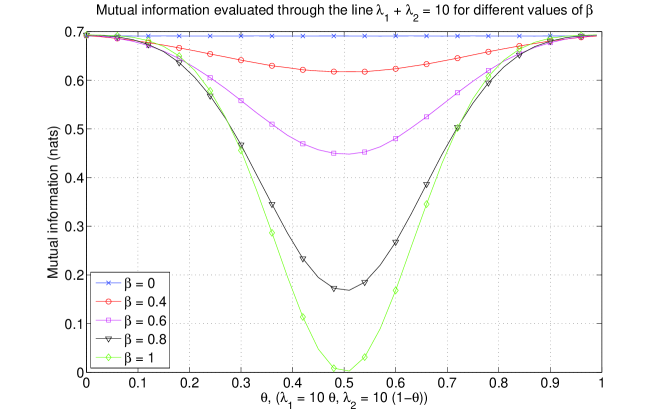
Figure 2: Graphical representation of the mutual information $I_{ce}(\lambda_{1},\lambda_{2},\beta)$ in the counterexample for different values of the channel parameter $\beta$ along the line $\lambda_{1}+\lambda_{2}=\rho=10$. It can be readily seen that, except for the case $\beta=0$, the function is not concave.

IV-D Concavity results summary

At the beginning of Section IV we have argued that the mutual information is concave with respect to the full transmitted signal covariance matrix $\mathbf{Q}$ for the case where the signaling is Gaussian and also for the low SNR regime. Next we have discussed that this result cannot be generalized for arbitrary signaling distributions because, in the general case, the mutual information is not well defined as a function of $\mathbf{Q}$ alone.

In Sections IV-A and IV-B, we have encountered two particular cases where the mutual information is a concave function. In the first case, we have seen that the mutual information is concave with respect to the SNR and, in the second, that the mutual information is a concave function of the squared singular values of the precoder, provided that the eigenvectors of the channel covariance $\mathbf{R}_{\boldsymbol{\mathbf{H}}}$ and the left singular vectors of the precoder $\mathbf{P}$ coincide. For the general case where these vectors do not coincide in general, we have shown in Section IV-C that the mutual information is not concave in the squared singular values.

A summary of the different concavity results for the mutual information as a function of the configuration of the linear vector Gaussian channel can be found in Table I.

TABLE I: Summary of the concavity type of the mutual information.
($\checkmark$ indicates concavity, $\times$ indicates non-concavity, and $-$ indicates that it does not apply)

	Scalar	Vector	Matrix
	Power, ${\sf snr}$,	Squared singular values, $\boldsymbol{\lambda}$,	Transmit covariance, $\mathbf{Q}$,
Cases	$\mathbf{P}=\sqrt{{\sf snr}}\mathbf{I}$	$\mathbf{P}=\mathbf{U}_{\mathbf{P}}\mathbf{Diag}\big{(}\sqrt{\boldsymbol{\lambda}})\mathbf{V}_{\mathbf{P}}^{\sf T}$	$\mathbf{Q}=\mathbf{P}\mathbf{R}_{\boldsymbol{S}}\mathbf{P}^{\sf T}$
General case: $\boldsymbol{Y}=\mathbf{H}\mathbf{P}\boldsymbol{S}+\boldsymbol{Z}$	$\checkmark$ [5] [10]	$\times$ (Section IV-C)	$-$ (Section III-E)
	(Section IV-A)
Channel covariance $\mathbf{R}_{\boldsymbol{\mathbf{H}}}$ and precoder $\mathbf{P}$	$\checkmark$	$\checkmark$ (Section IV-B)	$-$ (Section III-E)
share singular/eigenvectors: $\mathbf{U}_{\mathbf{P}}=\mathbf{U}_{\mathbf{H}}$
Independent parallel communication:	$\checkmark$	$\checkmark$ [17]	$\checkmark$ [17]
$\mathbf{R}_{\boldsymbol{\mathbf{H}}}=\mathbf{U}_{\mathbf{P}}=\mathbf{V}_{\mathbf{P}}=\mathbf{I}$, $P_{\boldsymbol{S}}=\prod_{i}P_{S_{i}}$			(Note that $\mathbf{Q}$ is diagonal)
Low SNR regime: $\mathbf{R}_{\boldsymbol{Z}}=N_{0}\mathbf{I}_{n}$, $N_{0}\gg 1$	$\checkmark$	$\checkmark$	$\checkmark$ [16]
Gaussian signaling: $\boldsymbol{S}=\boldsymbol{S}_{\mathcal{G}}$	$\checkmark$	$\checkmark$	$\checkmark$

V Multivariate extension of Costa’s entropy power inequality

Having proved that the mutual information and, hence, the differential entropy are concave functions of the squared singular values $\boldsymbol{\lambda}$ of the precoder $\mathbf{P}$ for the case where the left singular vectors of the precoder coincide with the eigenvectors of the channel covariance $\mathbf{R}_{\boldsymbol{\mathbf{H}}}$, ${{\sf H}}_{\boldsymbol{\lambda}}I(\boldsymbol{S};\boldsymbol{Y})={{\sf H}}_{\boldsymbol{\lambda}}h(\boldsymbol{Y})\leq\boldsymbol{0}$, we want to study if this last result can be strengthened by proving the concavity in $\boldsymbol{\lambda}$ of the entropy power.

The entropy power of the random vector $\boldsymbol{Y}\in\mathds{R}^{n}$ was first introduced by Shannon in his seminal work [18] and is, since then, defined as

$$N(\boldsymbol{Y})=\frac{1}{2\pi\textrm{e}}\exp\left(\frac{2}{n}h(\boldsymbol{Y})\right),$$ (107)

where $h(\boldsymbol{Y})$ represents the differential entropy as defined in (6). The entropy power of a random vector $\boldsymbol{Y}$ represents the variance (or power) of a standard Gaussian random vector $\boldsymbol{Y}_{\mathcal{G}}\sim\mathcal{N}\left(\boldsymbol{0},\sigma^{2}\mathbf{I}_{n}\right)$ such that both $\boldsymbol{Y}$ and $\boldsymbol{Y}_{\mathcal{G}}$ have identical differential entropy, $h(\boldsymbol{Y}_{\mathcal{G}})=h(\boldsymbol{Y})$.

Costa proved in [10] that, provided that the random vector $\boldsymbol{W}$ is white Gaussian distributed, then

$$N(\boldsymbol{X}+\sqrt{t}\boldsymbol{W})\geq(1-t)N(\boldsymbol{X})+tN(\boldsymbol{X}+\boldsymbol{W}),$$ (108)

where $t\in[0,1]$. As Costa noted, the above entropy power inequality (EPI) is equivalent to the concavity of the entropy power function $N(\boldsymbol{X}+\sqrt{t}\boldsymbol{W})$ with respect to the parameter $t$, or, formally

$$\frac{\operatorname*{d}\!^{2}}{\operatorname*{d}\!t^{2}}N\big{(}\boldsymbol{X}+\sqrt{t}\boldsymbol{W}\big{)}={{\sf H}}_{t}N\big{(}\boldsymbol{X}+\sqrt{t}\boldsymbol{W}\big{)}\leq 0.$$ (109)

Due to its inherent interest and to the fact that the proof by Costa was rather involved, simplified proofs of his result have been subsequently given in [19, 20, 21, 22].

Additionally, in his paper Costa presented two extensions of his main result in (109). Precisely, he showed that the EPI is also valid when the Gaussian vector $\boldsymbol{W}$ is not white, and also for the case where the $t$ parameter is multiplying the arbitrarily distributed random vector $\boldsymbol{X}$ instead:

$${{\sf H}}_{t}N\big{(}\sqrt{t}\boldsymbol{X}+\boldsymbol{W}\big{)}\leq 0.$$ (110)

Observe that $\sqrt{t}$ in (110) plays the role of a scalar precoder. We next consider an extension of (110) to the case where the scalar precoder $\sqrt{t}$ is replaced by a multivariate precoder $\mathbf{P}\in\mathds{R}^{p\times m}$ and a channel $\mathbf{H}\in\mathds{R}^{n\times p}$ for the particular case where the precoder left singular vectors coincide with the channel covariance eigenvectors. Similarly as in Section IV-B we assume that $m\geq p$. The case $m<p$ is presented after the proof of the following theorem.

Theorem 7 (Costa’s multivariate EPI)

Consider $\boldsymbol{Y}=\mathbf{H}\mathbf{P}\boldsymbol{S}+\boldsymbol{Z}$, where all the terms are defined as in Theorem 3, for the particular case where the eigenvectors of the channel covariance matrix $\mathbf{R}_{\boldsymbol{\mathbf{H}}}$ coincide with the left singular vectors of the precoder $\mathbf{P}\in\mathds{R}^{p\times m}$ and where we assume that $m\geq p$. It then follows that the entropy power $N(\boldsymbol{Y})$ is a concave function of $\boldsymbol{\lambda}$, i.e.,

$${{\sf H}}_{\boldsymbol{\lambda}}N(\boldsymbol{Y})\leq\boldsymbol{0}.$$

Moreover, the Hessian matrix of the entropy power function $N(\boldsymbol{Y})$ with respect to $\boldsymbol{\lambda}$ is given by

$${{\sf H}}_{\boldsymbol{\lambda}}N(\boldsymbol{Y})=\frac{N(\boldsymbol{Y})}{n}\mathbf{Diag}(\boldsymbol{\sigma})\left(\frac{\mathbf{diag}(\mathbf{E}_{\boldsymbol{\mathbf{V}_{\mathbf{P}}^{\sf T}S}})\mathbf{diag}(\mathbf{E}_{\boldsymbol{\mathbf{V}_{\mathbf{P}}^{\sf T}S}})^{\sf T}}{n}-{\sf E}\left\{\boldsymbol{\Phi}_{\boldsymbol{\mathbf{V}_{\mathbf{P}}^{\sf T}S}}(\boldsymbol{Y})\circ\boldsymbol{\Phi}_{\boldsymbol{\mathbf{V}_{\mathbf{P}}^{\sf T}S}}(\boldsymbol{Y})\right\}\right)\mathbf{Diag}(\boldsymbol{\sigma}),$$ (111)

where we recall that $\mathbf{diag}(\mathbf{E}_{\boldsymbol{\mathbf{V}_{\mathbf{P}}^{\sf T}S}})$ is a column vector with the diagonal entries of the matrix $\mathbf{E}_{\boldsymbol{\mathbf{V}_{\mathbf{P}}^{\sf T}S}}$.

Proof:

First, let us prove (111). From the definition of the entropy power in (107) and applying the chain rule for Hessians in (167) we obtain

$$\begin{split}{{\sf H}}_{\boldsymbol{\lambda}}N(\boldsymbol{Y})&={{\sf D}}_{\boldsymbol{\lambda}}^{\sf T}h(\boldsymbol{Y})\cdot{{\sf H}}_{h(\boldsymbol{Y})}N(\boldsymbol{Y})\cdot{{\sf D}}_{\boldsymbol{\lambda}}h(\boldsymbol{Y})+{{\sf D}}_{h(\boldsymbol{Y})}N(\boldsymbol{Y})\cdot{{\sf H}}_{\boldsymbol{\lambda}}h(\boldsymbol{Y})\\ &=\frac{2N(\boldsymbol{Y})}{n}\left(\frac{2{{\sf D}}_{\boldsymbol{\lambda}}^{\sf T}h(\boldsymbol{Y}){{\sf D}}_{\boldsymbol{\lambda}}h(\boldsymbol{Y})}{n}+{{\sf H}}_{\boldsymbol{\lambda}}h(\boldsymbol{Y})\right).\end{split}$$ (112)

Now, recalling from [5, Eq. (61)] that ${{\sf D}}_{\boldsymbol{\lambda}}^{\sf T}h(\boldsymbol{Y})=(1/2)\mathbf{Diag}(\boldsymbol{\sigma})\mathbf{diag}(\mathbf{E}_{\boldsymbol{\mathbf{V}_{\mathbf{P}}^{\sf T}S}})$ and incorporating the expression for ${{\sf H}}_{\boldsymbol{\lambda}}h(\boldsymbol{Y})$ calculated in Theorem 5, the result in (111) follows.

Now that a explicit expression for the Hessian matrix has been obtained, we wish to prove that it is negative semidefinite. Note from (112) that, except for the positive factor $2N(\boldsymbol{Y})/n$, the Hessian matrix ${{\sf H}}_{\boldsymbol{\lambda}}N(\boldsymbol{Y})$ is the sum of a rank one positive semidefinite matrix and the Hessian matrix of the differential entropy, which is negative semidefinite according to Theorem 5. Consequently, the definiteness of ${{\sf H}}_{\boldsymbol{\lambda}}N(\boldsymbol{Y})$ is, a priori, undetermined, and some further developments are needed to determine it, which is what we do next.

First consider the positive semidefinite matrix $\mathbf{A}(\boldsymbol{y})\in\mathds{S}^{p^{\prime}}_{+}$, which is obtained by selecting the first $p^{\prime}={\sf rank}(\mathbf{R}_{\boldsymbol{\mathbf{H}}})$ columns and rows of the positive semidefinite matrix $\mathbf{Diag}\big{(}\sqrt{\boldsymbol{\sigma}}\big{)}\boldsymbol{\Phi}_{\boldsymbol{\mathbf{V}_{\mathbf{P}}^{\sf T}S}}(\boldsymbol{y})\mathbf{Diag}\big{(}\sqrt{\boldsymbol{\sigma}}\big{)}$,

$$\left[\mathbf{A}(\boldsymbol{y})\right]_{ij}=\big{[}\mathbf{Diag}\big{(}\sqrt{\boldsymbol{\sigma}}\big{)}\boldsymbol{\Phi}_{\boldsymbol{\mathbf{V}_{\mathbf{P}}^{\sf T}S}}(\boldsymbol{Y})\mathbf{Diag}\big{(}\sqrt{\boldsymbol{\sigma}}\big{)}\big{]}_{ij},\quad\{i,j\}=1,\ldots,p^{\prime}.$$ (113)

With this definition, it is now easy to see that the expression

$$\frac{{\sf E}\left\{\mathbf{diag}(\mathbf{A}(\boldsymbol{y}))\right\}{\sf E}\bigl{\{}\mathbf{diag}(\mathbf{A}(\boldsymbol{y}))^{\sf T}\bigr{\}}}{n}-{\sf E}\bigl{\{}\mathbf{A}(\boldsymbol{y})\circ\mathbf{A}(\boldsymbol{y})\bigr{\}}$$ (114)

coincides (up to the factor $2N(\boldsymbol{Y})/n$) with the first $p^{\prime}$ rows and columns of the Hessian matrix ${{\sf H}}_{\boldsymbol{\lambda}}N(\boldsymbol{Y})$ in (111). Recalling that the remaining elements of the Hessian matrix ${{\sf H}}_{\boldsymbol{\lambda}}N(\boldsymbol{Y})$ are zero due to the presence of the matrix $\mathbf{Diag}(\boldsymbol{\sigma})$, it is sufficient to show that the expression in (114) is negative semidefinite to prove the negative semidefiniteness of ${{\sf H}}_{\boldsymbol{\lambda}}N(\boldsymbol{Y})$.

Now, we apply Proposition -G.9 to $\mathbf{A}(\boldsymbol{y})$, yielding

$$\mathbf{A}(\boldsymbol{y})\circ\mathbf{A}(\boldsymbol{y})\geq\frac{\mathbf{diag}(\mathbf{A}(\boldsymbol{y}))\mathbf{diag}(\mathbf{A}(\boldsymbol{y}))^{\sf T}}{p^{\prime}}.$$ (115)

Taking the expectation in both sides of (115), we have

$${\sf E}\left\{\mathbf{A}(\boldsymbol{Y})\circ\mathbf{A}(\boldsymbol{Y})\right\}\geq\frac{{\sf E}\left\{\mathbf{diag}(\mathbf{A}(\boldsymbol{Y}))\mathbf{diag}(\mathbf{A}(\boldsymbol{Y}))^{\sf T}\right\}}{p^{\prime}},$$ (116)

From Lemma -G.10 we know that

$${\sf E}\bigl{\{}\mathbf{diag}(\mathbf{A}(\boldsymbol{Y}))\mathbf{diag}(\mathbf{A}(\boldsymbol{Y}))^{\sf T}\bigr{\}}\geq{\sf E}\bigl{\{}\mathbf{diag}(\mathbf{A}(\boldsymbol{Y}))\bigr{\}}{\sf E}\bigl{\{}\mathbf{diag}(\mathbf{A}(\boldsymbol{Y}))^{\sf T}\bigr{\}},$$

from which it follows that

$${\sf E}\left\{\mathbf{A}(\boldsymbol{Y})\circ\mathbf{A}(\boldsymbol{Y})\right\}\geq\frac{{\sf E}\left\{\mathbf{diag}(\mathbf{A}(\boldsymbol{Y}))\right\}{\sf E}\left\{\mathbf{diag}(\mathbf{A}(\boldsymbol{Y}))^{\sf T}\right\}}{p^{\prime}}.$$

Since the operators $\mathbf{diag}(\mathbf{A})$ and expectation commute we finally obtain the desired result as

$${\sf E}\left\{\mathbf{A}(\boldsymbol{Y})\circ\mathbf{A}(\boldsymbol{Y})\right\}\geq\frac{\mathbf{diag}({\sf E}\left\{\mathbf{A}(\boldsymbol{Y})\right\})\mathbf{diag}({\sf E}\left\{\mathbf{A}(\boldsymbol{Y})\right\})^{\sf T}}{p^{\prime}}\geq\frac{\mathbf{diag}({\sf E}\left\{\mathbf{A}(\boldsymbol{Y})\right\})\mathbf{diag}({\sf E}\left\{\mathbf{A}(\boldsymbol{Y})\right\})^{\sf T}}{n},$$

where in last inequality we have used that $p^{\prime}={\sf rank}(\mathbf{R}_{\boldsymbol{\mathbf{H}}})\leq\min\{n,p\}\leq n$, as $\mathbf{R}_{\boldsymbol{\mathbf{H}}}=\mathbf{H}^{\sf T}\mathbf{R}_{\boldsymbol{Z}}^{-1}\mathbf{H}$ and $\mathbf{H}\in\mathds{R}^{n\times p}$. ∎

Remark 9

For the case where $m<p$, we assume that the matrix $\mathbf{U}_{\mathbf{P}}\in\mathds{R}^{p\times m}$ contains the $m$ eigenvectors in $\mathbf{U}_{\mathbf{H}}$ associated with the $m$ largest eigenvalues of $\mathbf{R}_{\boldsymbol{\mathbf{H}}}$. It then follows that the Hessian matrix ${{\sf H}}_{\boldsymbol{\lambda}}N(\boldsymbol{Y})$ is also negative semidefinite and its expression is the same given in (111) by simply replacing $\boldsymbol{\sigma}$ by $\boldsymbol{\tilde{\sigma}}=(\sigma_{1}\ldots\sigma_{m})^{\sf T}$.

Remark 10

For the case where $\mathbf{R}_{\boldsymbol{\mathbf{H}}}=\mathbf{I}_{p}$ and $p=m$ we recover our results in [23].

Another possibility of multivariate generalization of Costa’s EPI would be to study the concavity of $N(\boldsymbol{X}+\boldsymbol{Z})$ with respect to the covariance of the noise vector $\mathbf{R}_{\boldsymbol{Z}}$. Numerical computations seem to indicate that the entropy power is indeed concave in $\mathbf{R}_{\boldsymbol{Z}}$. However, a proof has been elusive, mainly due to the fact that, differently from the conditional MSE, $\boldsymbol{\Phi}_{\boldsymbol{S}}(\boldsymbol{y})$, the conditional Fisher information matrix $\boldsymbol{\Gamma}_{\boldsymbol{Y}}(\boldsymbol{y})$, which appears when differentiating with respect to $\mathbf{R}_{\boldsymbol{Z}}$, is not a positive definite function $\forall\boldsymbol{y}$.

VI Extensions to the complex field

So far, the presented results hold for the case where all the variables and parameters take values from the field of real numbers. Due to the simplicity of working with baseband equivalent models, it is a common practice when studying communication systems to model the parameters and random variables in the complex field, and work with the following complex linear vector Gaussian channel:

$$\boldsymbol{Y}_{c}=\mathbf{G}_{c}\boldsymbol{S}_{c}+\boldsymbol{Z}_{c},$$ (117)

where $\mathbf{G}_{c}\in\mathds{C}^{n\times m}$ and all the other dimensions are defined accordingly and the noise $\boldsymbol{Z}_{c}$ is a zero mean circularly symmetric (or proper [24]) complex Gaussian random vector with covariance ${\sf E}\left\{\boldsymbol{Z}_{c}\boldsymbol{Z}_{c}^{\dagger}\right\}={\mathbf{R}_{\boldsymbol{Z}}}_{c}$. The complex model in (117) can be equivalently rewritten by defining an extended double-dimensional real model of (117). We consider the extended vectors and matrices

$$\boldsymbol{Y}_{r}=\left[\begin{array}[]{c}\Re\textrm{e}\boldsymbol{Y}_{c}\\ \Im\textrm{m}\boldsymbol{Y}_{c}\end{array}\right],\>\mathbf{G}_{r}=\left[\begin{array}[]{cc}\Re\textrm{e}\mathbf{G}_{c}&-\Im\textrm{m}\mathbf{G}_{c}\\ \Im\textrm{m}\mathbf{G}_{c}&\Re\textrm{e}\mathbf{G}_{c}\end{array}\right],\>\boldsymbol{S}_{r}=\left[\begin{array}[]{c}\Re\textrm{e}\boldsymbol{S}_{c}\\ \Im\textrm{m}\boldsymbol{S}_{c}\end{array}\right],\>\boldsymbol{Z}_{r}=\left[\begin{array}[]{c}\Re\textrm{e}\boldsymbol{Z}_{c}\\ \Im\textrm{m}\boldsymbol{Z}_{c}\end{array}\right],$$ (126)

and then rewrite the input-output relation in (117) according to the real model

$$\boldsymbol{Y}_{r}=\mathbf{G}_{r}\boldsymbol{S}_{r}+\boldsymbol{Z}_{r}.$$ (127)

With these definitions, we have that, for example, $h(\boldsymbol{Y}_{c})=h(\boldsymbol{Y}_{r})$ or $I(\boldsymbol{S}_{c};\boldsymbol{Y}_{c})=I(\boldsymbol{S}_{r};\boldsymbol{Y}_{r})$ [24].

Working with the real model in (127), it is possible to calculate, for example, the Jacobian of the mutual information with respect to the complex precoder $\mathbf{G}_{c}$ by using the results for the real case and the chain rule as

$${{\sf D}}_{\mathbf{G}_{c}}I(\boldsymbol{S}_{c};\boldsymbol{Y}_{c})={{\sf D}}_{\mathbf{G}_{c}}I(\boldsymbol{S}_{r};\boldsymbol{Y}_{r}) \triangleq\frac{1}{2}\big{(}{{\sf D}}_{\Re\textrm{e}\mathbf{G}_{c}}I(\boldsymbol{S}_{r};\boldsymbol{Y}_{r})-\textrm{j}{{\sf D}}_{\Im\textrm{m}\mathbf{G}_{c}}I(\boldsymbol{S}_{r};\boldsymbol{Y}_{r})\big{)}$$ (128)

$$=\frac{1}{2}\big{(}{{\sf D}}_{\mathbf{G}_{r}}I(\boldsymbol{S}_{r};\boldsymbol{Y}_{r}){{\sf D}}_{\Re\textrm{e}\mathbf{G}_{c}}\mathbf{G}_{r}-\textrm{j}{{\sf D}}_{\mathbf{G}_{r}}I(\boldsymbol{S}_{r};\boldsymbol{Y}_{r}){{\sf D}}_{\Im\textrm{m}\mathbf{G}_{c}}\mathbf{G}_{r}\big{)},$$ (129)

where we have used the convention for the complex derivative defined in [25] and where the Jacobians ${{\sf D}}_{\Re\textrm{e}\mathbf{G}_{c}}\mathbf{G}_{r}$ and ${{\sf D}}_{\Im\textrm{m}\mathbf{G}_{c}}\mathbf{G}_{r}$ can be found using the definition in (126) and the results in [15, Chapter 9]. Similarly, expressions for ${{\sf H}}_{\mathbf{G}_{c}}I(\boldsymbol{S}_{c};\boldsymbol{Y}_{c})$ or ${{\sf H}}_{\mathbf{G}_{c}^{*}}I(\boldsymbol{S}_{c};\boldsymbol{Y}_{c})$ can also be obtained by successive application of the complex derivative definition and the chain rule.

In the following we present a simplified complex counterpart of the Hessian result in Theorem 5 for the real case, which, despite its simplicity, illustrates the particularities of the complex case.

Theorem 8 (Mutual information Hessian in the complex case)

Consider the complex signal model $\boldsymbol{Y}_{c}=\mathbf{Diag}\big{(}\sqrt{\boldsymbol{\lambda}_{c}}\big{)}\boldsymbol{S}_{c}+\boldsymbol{W}_{c}$, where $\mathbf{Diag}\big{(}\sqrt{\boldsymbol{\lambda}_{c}}\big{)}\in\mathds{S}^{n}_{+}$ is an arbitrary deterministic diagonal matrix ($\boldsymbol{\lambda}_{c}\in\mathds{R}^{n}$), the signaling $\boldsymbol{S}_{c}\in\mathds{C}^{n}$ is arbitrarily distributed, and the noise vector $\boldsymbol{W}_{c}\in\mathds{C}^{n}$ follows a white Gaussian proper distribution and is independent of the input $\boldsymbol{S}_{c}$. Then, the differential entropy of the output vector $\boldsymbol{Y}_{c}$, $h(\boldsymbol{Y})$, satisfies

$${{\sf H}}_{\boldsymbol{\lambda}_{c}}h(\boldsymbol{Y}_{c})=-{\sf E}\left\{\boldsymbol{\Phi}_{\boldsymbol{S}_{c}}(\boldsymbol{Y})\circ\boldsymbol{\Phi}^{*}_{\boldsymbol{S}_{c}}(\boldsymbol{Y})+\overline{\boldsymbol{\Phi}}_{\boldsymbol{S}_{c}}(\boldsymbol{Y})\circ\overline{\boldsymbol{\Phi}}^{*}_{\boldsymbol{S}_{c}}(\boldsymbol{Y})\right\},$$ (130)

where we have defined

$$\boldsymbol{\Phi}_{\boldsymbol{S}_{c}}(\boldsymbol{y}) ={\sf E}\left\{\left(\boldsymbol{S}_{c}-{\sf E}\left\{\boldsymbol{S}_{c}\,\middle|\,\boldsymbol{y}\right\}\right)\left(\boldsymbol{S}_{c}-{\sf E}\left\{\boldsymbol{S}_{c}\,\middle|\,\boldsymbol{y}\right\}\right)^{\dagger}\,\middle|\,\boldsymbol{y}\right\}$$ (131)

$$\overline{\boldsymbol{\Phi}}_{\boldsymbol{S}_{c}}(\boldsymbol{y}) ={\sf E}\left\{\left(\boldsymbol{S}_{c}-{\sf E}\left\{\boldsymbol{S}_{c}\,\middle|\,\boldsymbol{y}\right\}\right)\left(\boldsymbol{S}_{c}-{\sf E}\left\{\boldsymbol{S}_{c}\,\middle|\,\boldsymbol{y}\right\}\right)^{\sf T}\,\middle|\,\boldsymbol{y}\right\}.$$ (132)

Proof:

The real extended model of $\boldsymbol{Y}_{c}=\mathbf{Diag}\big{(}\sqrt{\boldsymbol{\lambda}_{c}}\big{)}\boldsymbol{S}_{c}+\boldsymbol{W}_{c}$ is readily obtained as

$$\boldsymbol{Y}_{r}=\mathbf{Diag}\big{(}\sqrt{\boldsymbol{\lambda}_{r}}\big{)}\boldsymbol{S}_{r}+\boldsymbol{N}_{r}=\left[\begin{array}[]{cc}\mathbf{Diag}\big{(}\sqrt{\boldsymbol{\lambda}_{c}}\big{)}&\boldsymbol{0}\\ \boldsymbol{0}&\mathbf{Diag}\big{(}\sqrt{\boldsymbol{\lambda}_{c}}\big{)}\end{array}\right]\left[\begin{array}[]{c}\Re\textrm{e}\boldsymbol{S}_{c}\\ \Im\textrm{m}\boldsymbol{S}_{c}\end{array}\right]+\frac{1}{\sqrt{2}}\boldsymbol{W}_{r},$$ (137)

where now we have ${\sf E}\bigl{\{}\boldsymbol{W}_{r}\boldsymbol{W}_{r}^{\sf T}\bigr{\}}=\mathbf{I}_{2n}$.

Now, applying the chain rule for $\boldsymbol{\lambda}_{r}^{\sf T}=\big{[}\boldsymbol{\lambda}_{c}^{\sf T}\>\boldsymbol{\lambda}_{c}^{\sf T}\big{]}$ the elements of the Hessian matrix read as

$$\left[{{\sf H}}_{\boldsymbol{\lambda}_{c}}h(\boldsymbol{Y}_{c})\right]_{ij}=\frac{\partial^{2}h(\boldsymbol{Y}_{c})}{\partial\lambda_{c,i}\partial\lambda_{c,j}}=\frac{\partial^{2}h(\boldsymbol{Y}_{r})}{\partial\lambda_{r,i}\partial\lambda_{r,j}}+\frac{\partial^{2}h(\boldsymbol{Y}_{r})}{\partial\lambda_{r,i+n}\partial\lambda_{r,j}}+\frac{\partial^{2}h(\boldsymbol{Y}_{r})}{\partial\lambda_{r,i}\partial\lambda_{r,j+n}}+\frac{\partial^{2}h(\boldsymbol{Y}_{r})}{\partial\lambda_{r,i+n}\partial\lambda_{r,j+n}}.$$

The four terms in the complex Hessian can be identified with the elements of the Hessian for the real case, which thanks to Theorem 5 can be written as

$$\frac{\partial^{2}h(\boldsymbol{Y}_{r})}{\partial\lambda_{r,i}\partial\lambda_{r,j}}=-2{\sf E}\left\{\left({\sf E}\left\{\left(S_{r,i}-{\sf E}\left\{S_{r,i}\,\middle|\,\boldsymbol{Y}\right\}\right)\left(S_{r,j}-{\sf E}\left\{S_{r,j}\,\middle|\,\boldsymbol{Y}\right\}\right)\,\middle|\,\boldsymbol{Y}\right\}\right)^{2}\right\}.$$ (138)

Noting that $S_{r,i}=\Re\textrm{e}S_{c,i}$ and $S_{r,i+n}=\Im\textrm{m}S_{c,i}$, we can finally write

$$\left[{{\sf H}}_{\boldsymbol{\lambda}_{c}}h(\boldsymbol{Y}_{c})\right]_{ij}= -2{\sf E}\left\{\left({\sf E}\left\{\Re\textrm{e}\left(S_{c,i}-{\sf E}\left\{S_{c,i}\,\middle|\,\boldsymbol{Y}\right\}\right)\Re\textrm{e}\left(S_{c,j}-{\sf E}\left\{S_{c,j}\,\middle|\,\boldsymbol{Y}\right\}\right)\,\middle|\,\boldsymbol{Y}\right\}\right)^{2}\right\}$$ (139)

$$-2{\sf E}\left\{\left({\sf E}\left\{\Re\textrm{e}\left(S_{c,i}-{\sf E}\left\{S_{c,i}\,\middle|\,\boldsymbol{Y}\right\}\right)\Im\textrm{m}\left(S_{c,j}-{\sf E}\left\{S_{c,j}\,\middle|\,\boldsymbol{Y}\right\}\right)\,\middle|\,\boldsymbol{Y}\right\}\right)^{2}\right\}$$ (140)

$$-2{\sf E}\left\{\left({\sf E}\left\{\Im\textrm{m}\left(S_{c,i}-{\sf E}\left\{S_{c,i}\,\middle|\,\boldsymbol{Y}\right\}\right)\Re\textrm{e}\left(S_{c,j}-{\sf E}\left\{S_{c,j}\,\middle|\,\boldsymbol{Y}\right\}\right)\,\middle|\,\boldsymbol{Y}\right\}\right)^{2}\right\}$$ (141)

$$-2{\sf E}\left\{\left({\sf E}\left\{\Im\textrm{m}\left(S_{c,i}-{\sf E}\left\{S_{c,i}\,\middle|\,\boldsymbol{Y}\right\}\right)\Im\textrm{m}\left(S_{c,j}-{\sf E}\left\{S_{c,j}\,\middle|\,\boldsymbol{Y}\right\}\right)\,\middle|\,\boldsymbol{Y}\right\}\right)^{2}\right\}.$$ (142)

Now, with the definitions in (132) and (131) and a slight amount of algebra, the result follows. ∎

It is important to highlight that, whereas in the real case the conditional MMSE matrix $\boldsymbol{\Phi}_{\boldsymbol{S}}(\boldsymbol{y})$ was enough to compute the Hessian, in the complex case, in addition to the conditional MMSE matrix (as defined in (131)) there is an extra matrix $\overline{\boldsymbol{\Phi}}_{\boldsymbol{S}_{c}}(\boldsymbol{y})$ defined as in (132), and which is referred to as the conditional pseudo-MMSE matrix.

-A The commutation $\mathbf{K}_{q,r}$, symmetrization $\mathbf{N}_{q}$, duplication $\mathbf{D}_{q}$, and reduction $\mathbf{S}_{q}$ matrices.

In this appendix we present four matrices that are very important when calculating Hessian matrices. The definitions of the commutation $\mathbf{K}_{q,r}$, symmetrization $\mathbf{N}_{q}$, and duplication $\mathbf{D}_{q}$ matrices have been taken from [15] and the reduction matrix $\mathbf{S}_{q}$ has been defined by the authors of the present work.

Given any matrix $\mathbf{A}\in\mathds{R}^{q\times r}$, the two vectors ${\sf vec}\mathbf{A}$ and ${\sf vec}\mathbf{A}^{\!{\sf T}}$ contain the same elements but arranged in a different order. Consequently, there exists a unique permutation matrix $\mathbf{K}_{q,r}\in\mathds{R}^{qr\times qr}$ independent of $\mathbf{A}$, which is called commutation matrix, that satisfies

$${\sf vec}\mathbf{A}^{\!{\sf T}}=\mathbf{K}_{q,r}{\sf vec}\mathbf{A},\quad\textrm{and}\quad\mathbf{K}_{q,r}^{\sf T}=\mathbf{K}_{q,r}^{-1}=\mathbf{K}_{r,q}.$$ (143)

It is easy to verify that the entries of the commutation matrix satisfy

$$\left[\mathbf{K}_{q,r}\right]_{i+(j-1)r,i^{\prime}+(j^{\prime}-1)q}=\delta_{i^{\prime}j}\delta_{j^{\prime}i},\quad\{i^{\prime},j\}\in[1,q],\quad\{i,j^{\prime}\}\in[1,r].$$ (144)

The main reason why we have introduced the commutation matrix is due to the property from which it obtains its name, as it enables us to commute the two matrices of a Kronecker product [15, Theorem 3.9],

$$\mathbf{K}_{s,q}(\mathbf{A}\otimes\mathbf{B})=(\mathbf{B}\otimes\mathbf{A})\mathbf{K}_{t,r},$$ (145)

where we have considered $\mathbf{A}\in\mathds{R}^{q\times r}$ and $\mathbf{B}\in\mathds{R}^{s\times t}$.

We also define $\mathbf{K}_{q}=\mathbf{K}_{q,q}$ for the case where the commutation matrix is square. An important property of the square matrix $\mathbf{K}_{q}$ is given in the following lemma.

Lemma -A.1

Let $\mathbf{A}\in\mathds{R}^{q\times r}$ and $\mathbf{B}\in\mathds{R}^{q\times t}$. Then,

$$\begin{split}\left[\mathbf{A}\otimes\mathbf{B}\right]_{i+(j-1)q,k+(l-1)t}&=\mathbf{A}_{jl}\mathbf{B}_{ik},\\ \left[\mathbf{K}_{q}(\mathbf{A}\otimes\mathbf{B})\right]_{i+(j-1)q,k+(l-1)t}&=\mathbf{A}_{il}\mathbf{B}_{jk},\end{split}\quad\quad\{i,j\}\in[1,q],\quad k\in[1,t],\quad l\in[1,r],$$ (146)

Proof:

The equality for the entries of the product $\mathbf{A}\otimes\mathbf{B}$ follows straightforwardly from the definition [26, Section 4.2]. Concerning the entries of $\mathbf{K}_{q}(\mathbf{A}\otimes\mathbf{B})$, we have

$$\left[\mathbf{K}_{q}(\mathbf{A}\otimes\mathbf{B})\right]_{i+(j-1)q,k+(l-1)t} =\sum_{i^{\prime}=1}^{q}\sum_{j^{\prime}=1}^{q}\left[\mathbf{K}_{q}\right]_{i+(j-1)q,i^{\prime}+(j^{\prime}-1)q}\left[\mathbf{A}\otimes\mathbf{B}\right]_{i^{\prime}+(j^{\prime}-1)q,k+(l-1)t}$$ (147)

$$=\sum_{i^{\prime}=1}^{q}\sum_{j^{\prime}=1}^{q}\delta_{i^{\prime}j}\delta_{j^{\prime}i}\mathbf{A}_{j^{\prime}l}\mathbf{B}_{i^{\prime}k}$$ (148)

$$=\mathbf{A}_{il}\mathbf{B}_{jk},$$ (149)

where we have used the expression for the elements of $\mathbf{K}_{q}$ in (144). ∎

When calculating Jacobian and Hessian matrices, the form $\mathbf{I}_{q}+\mathbf{K}_{q}$ is usually encountered. Hence, we define the symmetrization matrix $\mathbf{N}_{q}=\tfrac{1}{2}(\mathbf{I}_{q}+\mathbf{K}_{q})$, which is singular and has the following properties

$$\mathbf{N}_{q} =\mathbf{N}_{q}^{\sf T}=\mathbf{N}_{q}^{2}$$ (150)

$$\mathbf{N}_{q} =\mathbf{N}_{q}\mathbf{K}_{q}=\mathbf{K}_{q}\mathbf{N}_{q}.$$ (151)

The name of the symmetrization matrix comes from the fact that given any square matrix $\mathbf{A}\in\mathds{R}^{q\times q}$, then

$$\mathbf{N}_{q}{\sf vec}\mathbf{A}=\tfrac{1}{2}\big{(}{\sf vec}\mathbf{A}+{\sf vec}\mathbf{A}^{\!{\sf T}}\big{)}=\tfrac{1}{2}{\sf vec}\big{(}\mathbf{A}+\mathbf{A}^{\!{\sf T}}\big{)}.$$ (152)

The last important property of the symmetrization matrix is

$$\mathbf{N}_{q}(\mathbf{A}\otimes\mathbf{A})=(\mathbf{A}\otimes\mathbf{A})\mathbf{N}_{q},$$ (153)

which follows from the definition $\mathbf{N}_{q}=\tfrac{1}{2}(\mathbf{I}_{q}+\mathbf{K}_{q})$ together with (145).

Another important matrix related to the calculation of Jacobian and Hessian matrices, specially when symmetric matrices are involved, is the duplication matrix $\mathbf{D}_{q}$. Given any symmetric matrix $\mathbf{R}\in\mathds{S}^{q}$, we denote by ${\sf vech}\mathbf{R}$ the $\tfrac{1}{2}q(q+1)$-dimensional vector that is obtained from ${\sf vec}\mathbf{R}$ by eliminating all the repeated elements that lie strictly above the diagonal of $\mathbf{R}$. Then, the duplication matrix $\mathbf{D}_{q}\in\mathds{R}^{q^{2}\times\tfrac{1}{2}q(q+1)}$ fulfills [15, Section 3.8]

$${\sf vec}\mathbf{R}=\mathbf{D}_{q}{\sf vech}\mathbf{R},$$ (154)

for any $q$-dimensional symmetric matrix $\mathbf{R}$. The duplication matrix takes its name from the fact that it duplicates the entries of ${\sf vech}\mathbf{R}$ which correspond to off-diagonal elements of $\mathbf{R}$ to produce the elements of ${\sf vec}\mathbf{R}$.

Since $\mathbf{D}_{q}$ has full column rank, it is possible to invert the transformation in (154) to obtain

$${\sf vech}\mathbf{R}=\mathbf{D}_{q}^{\textrm{\footnotesize{+}}}{\sf vec}\mathbf{R}=\big{(}\mathbf{D}_{q}^{\sf T}\mathbf{D}_{q}\big{)}^{-1}\mathbf{D}_{q}^{\sf T}{\sf vec}\mathbf{R}.$$ (155)

The most important properties of the duplication matrix are [15, Theorem 3.12]

$$\mathbf{K}_{q}\mathbf{D}_{q}=\mathbf{D}_{q},\quad\mathbf{N}_{q}\mathbf{D}_{q}=\mathbf{D}_{q},\quad\mathbf{D}_{q}\mathbf{D}_{q}^{\textrm{\footnotesize{+}}}=\mathbf{N}_{q},\quad\mathbf{D}_{q}^{\textrm{\footnotesize{+}}}\mathbf{N}_{q}=\mathbf{D}_{q}^{\textrm{\footnotesize{+}}}.$$ (156)

The last one of the matrices introduced in this appendix is the reduction matrix $\mathbf{S}_{q}\in\mathds{R}^{q^{2}\times q}$. The entries of the reduction matrix are defined as

$$[\mathbf{S}_{q}]_{i+(j-1)q,k}=\delta_{ij}\delta_{ik}=\delta_{ijk},\quad\{i,j,k\}\in[1,q]$$ (157)

from which it is easy to verify that the reduction matrix fulfills

$$\mathbf{K}_{q}\mathbf{S}_{q}=\mathbf{S}_{q},\quad\mathbf{N}_{q}\mathbf{S}_{q}=\mathbf{S}_{q}.$$ (158)

However, the most important property of the reduction matrix is that it can be used to reduce the Kronecker product of two matrices to their Schur product as it is detailed in the next lemma.

Lemma -A.2

Let $\mathbf{A}\in\mathds{R}^{q\times r}$, $\mathbf{B}\in\mathds{R}^{q\times r}$. Then,

$$\mathbf{S}_{q}^{\sf T}(\mathbf{A}\otimes\mathbf{B})\mathbf{S}_{r}=\mathbf{S}_{q}^{\sf T}(\mathbf{B}\otimes\mathbf{A})\mathbf{S}_{r}=\mathbf{A}\circ\mathbf{B}.$$ (159)

Proof:

From the expression for the elements of the Kronecker product in Lemma -A.1 and the expression for the elements of the reduction matrix we have that, for any $i\in[1,q]$ and $j\in[1,r]$,

$$\big{[}\mathbf{S}_{q}^{\sf T}(\mathbf{A}\otimes\mathbf{B})\mathbf{S}_{r}\big{]}_{i,j} =\sum_{k,l}^{q}\sum_{k^{\prime},l^{\prime}}^{r}[\mathbf{S}_{q}]_{k+(l-1)q,i}[\mathbf{A}\otimes\mathbf{B}]_{k+(l-1)q,k^{\prime}+(l^{\prime}-1)r}[\mathbf{S}_{r}]_{k^{\prime}+(l^{\prime}-1)r,j}$$ (160)

$$=\sum_{k,l}^{q}\sum_{k^{\prime},l^{\prime}}^{r}\mathbf{A}_{ll^{\prime}}\mathbf{B}_{kk^{\prime}}\delta_{kli}\delta_{k^{\prime}l^{\prime}j}$$ (161)

$$=\mathbf{A}_{ij}\mathbf{B}_{ij},$$ (162)

from which the result in the lemma follows. ∎

Finally, to conclude this appendix, we present two basic lemmas concerning the Kronecker product and the ${\sf vec}$ operator.

Lemma -A.3

Let $\mathbf{A}$, $\mathbf{B}$, $\mathbf{F}$, and $\mathbf{T}$ be four matrices such that the products $\mathbf{A}\mathbf{B}$ and $\mathbf{F}\mathbf{T}$ are defined. Then, $(\mathbf{A}\otimes\mathbf{F})(\mathbf{B}\otimes\mathbf{T})=\mathbf{A}\mathbf{B}\otimes\mathbf{F}\mathbf{T}$.

Proof:

See [15, Chapter 2]. ∎

Lemma -A.4

Let $\mathbf{A}$, $\mathbf{T}$, and $\mathbf{B}$ be three matrices such that the product $\mathbf{A}\mathbf{T}\mathbf{B}$ is defined. Then,

$${\sf vec}(\mathbf{A}\mathbf{T}\mathbf{B})=\big{(}\mathbf{B}^{\sf T}\otimes\mathbf{A}\big{)}{\sf vec}\mathbf{T}.$$ (163)

Proof:

See [15, Theorem 2.2] or [27, Proposition 7.1.6]. ∎

-B Conventions used for Jacobian and Hessian matrices

In this work we make extensive use of differentiation of matrix functions $\boldsymbol{\Psi}$ with respect to a matrix argument $\mathbf{T}$. From the many possibilities of displaying the partial derivatives $\partial^{r}\boldsymbol{\Psi}_{st}/\partial\mathbf{T}_{ij}\cdots\partial\mathbf{T}_{kl}$, we will stick to the “good notation” introduced by Magnus and Neudecker in [15, Section 9.4] which is briefly reproduced next for the sake of completeness.

Definition -B.1

Let $\boldsymbol{\Psi}$ be a differentiable $q\times t$ real matrix function of an $r\times s$ matrix of real variables $\mathbf{T}$. The Jacobian matrix of $\boldsymbol{\Psi}$ at $\mathbf{T}=\mathbf{T}_{0}$ is the $qt\times rs$ matrix

$${{\sf D}}_{\mathbf{T}}\boldsymbol{\Psi}(\mathbf{T}_{0})=\left.\frac{\partial\,{\sf vec}\,\boldsymbol{\Psi}(\mathbf{T})}{\partial({\sf vec}\mathbf{T})^{\sf T}}\right|_{\mathbf{T}=\mathbf{T}_{0}}.$$ (164)

Remark -B.2

To properly deal with the case where $\boldsymbol{\Psi}$ is a symmetric matrix, the ${\sf vec}$ operator in the numerator in (164) has to be replaced by a ${\sf vech}$ operator to avoid obtaining repeated elements. Similarly, ${\sf vech}$ has to replace ${\sf vec}$ in the denominator in (164) for the case where $\mathbf{T}$ is a symmetric matrix. For practical purposes, it is enough to calculate the Jacobian without taking into account any symmetry properties and then add a left factor $\mathbf{D}_{q}^{\textrm{\footnotesize{+}}}$ to the obtained Jacobian when $\boldsymbol{\Psi}$ is symmetric and/or a right factor $\mathbf{D}_{r}$ when $\mathbf{T}$ is symmetric. This proceeding will become more clear in the examples given below.

Definition -B.3

Let $\boldsymbol{\Psi}$ be a twice differentiable $q\times t$ real matrix function of an $r\times s$ matrix of real variables $\mathbf{T}$. The Hessian matrix of $\boldsymbol{\Psi}$ at $\mathbf{T}=\mathbf{T}_{0}$ is the $qtrs\times rs$ matrix

$${{\sf H}}_{\mathbf{T}}\boldsymbol{\Psi}(\mathbf{T}_{0})=\left.{{\sf D}}_{\mathbf{T}}\big{(}{{\sf D}}_{\mathbf{T}}^{\sf T}\boldsymbol{\Psi}(\mathbf{T})\big{)}\right|_{\mathbf{T}=\mathbf{T}_{0}}=\left.\frac{\partial}{\partial({\sf vec}\mathbf{T})^{\sf T}}{\sf vec}\left(\frac{\partial\,{\sf vec}\,\boldsymbol{\Psi}(\mathbf{T})}{\partial({\sf vec}\mathbf{T})^{\sf T}}\right)^{\!\!{\sf T}}\right|_{\mathbf{T}=\mathbf{T}_{0}}.$$ (165)

One can verify that the obtained Hessian matrix for the matrix function $\boldsymbol{\Psi}$ is the stacking of the $qt$ Hessian matrices corresponding to each individual element of vector ${\sf vec}\boldsymbol{\Psi}$.

Remark -B.4

Similarly to the Jacobian case, when $\boldsymbol{\Psi}$ or $\mathbf{T}$ are symmetric matrices, the ${\sf vech}$ operator has to replace the ${\sf vec}$ operator where appropriate in (165).

One of the major advantages of using the notation of [15] is that a simple chain rule can be applied for both the Jacobian and Hessian matrices, as detailed in the following lemma.

Lemma -B.5 ([15, Theorems 5.8 and 6.9])

Let $\boldsymbol{\Upsilon}$ be a twice differentiable $u\times v$ real matrix function of a $q\times t$ real matrix argument. Let $\boldsymbol{\Psi}$ be a twice differentiable $q\times t$ real matrix function of an $r\times s$ matrix of real variables $\mathbf{T}$. Define $\boldsymbol{\Omega}(\mathbf{T})=\boldsymbol{\Upsilon}(\boldsymbol{\Psi}(\mathbf{T}))$. The Jacobian and Hessian matrices of $\boldsymbol{\Omega}(\mathbf{T})$ at $\mathbf{T}=\mathbf{T}_{0}$ are:

$${{\sf D}}_{\mathbf{T}}\boldsymbol{\Omega}(\mathbf{T}_{0}) =({{\sf D}}_{\boldsymbol{\Psi}}\boldsymbol{\Upsilon}(\boldsymbol{\Psi}_{0}))({{\sf D}}_{\mathbf{T}}\boldsymbol{\Psi}(\mathbf{T}_{0}))$$ (166)

$${{\sf H}}_{\mathbf{T}}\boldsymbol{\Omega}(\mathbf{T}_{0}) =(\mathbf{I}_{uv}\otimes{{\sf D}}_{\mathbf{T}}\boldsymbol{\Psi}(\mathbf{T}_{0}))^{\sf T}{{\sf H}}_{\boldsymbol{\Psi}}\boldsymbol{\Upsilon}(\boldsymbol{\Psi}_{0})({{\sf D}}_{\mathbf{T}}\boldsymbol{\Psi}(\mathbf{T}_{0}))+({{\sf D}}_{\boldsymbol{\Psi}}\boldsymbol{\Upsilon}(\boldsymbol{\Psi}_{0})\otimes\mathbf{I}_{rs}){{\sf H}}_{\mathbf{T}}\boldsymbol{\Psi}(\mathbf{T}_{0}),$$ (167)

where $\boldsymbol{\Psi}_{0}=\boldsymbol{\Psi}(\mathbf{T}_{0})$.

The notation introduced above unifies the study of scalar $(q=t=1)$, vector $(t=1)$, and matrix functions of scalar $(r=s=1)$, vector $(s=1)$, or matrix arguments into the study of vector functions of vector arguments through the use of the ${\sf vec}$ and ${\sf vech}$ operators. However, the idea of arranging the partial derivatives of a scalar function of a matrix argument $\psi(\mathbf{T})$ into a matrix rather than a vector is quite appealing and sometimes useful, so we will also make use of the notation described next.

Definition -B.6

Let $\psi$ be differentiable scalar function of an $r\times s$ matrix of real variables $\mathbf{T}$. The gradient of $\psi$ at $\mathbf{T}=\mathbf{T}_{0}$ is the $r\times s$ matrix

$$\nabla_{\mathbf{T}}\psi(\mathbf{T}_{0})=\left.\frac{\partial\psi}{\partial\mathbf{T}}\right|_{\mathbf{T}=\mathbf{T}_{0}}.$$ (168)

It is easy to verify that ${{\sf D}}_{\mathbf{T}}\psi(\mathbf{T}_{0})={\sf vec}^{\sf T}\nabla_{\mathbf{T}}\psi(\mathbf{T}_{0})$.

We now give expressions for the most common Jacobian and Hessian matrices encountered during our developments.

Lemma -B.7

Consider $\mathbf{A}\in\mathds{R}^{q\times r}$, $\mathbf{T}\in\mathds{R}^{r\times s}$, $\mathbf{B}\in\mathds{R}^{s\times t}$, $\mathbf{R}\in\mathds{S}^{s}_{+}$, and $\mathbf{f}\in\mathds{R}^{r\times 1}$, such that $\mathbf{f}$ is a function of $\mathbf{T}$. Then, the following holds:

1. If $\boldsymbol{\Psi}=\mathbf{A}\mathbf{T}\mathbf{B}$, we have ${{\sf D}}_{\mathbf{T}}\boldsymbol{\Psi}=\big{(}\mathbf{B}^{\sf T}\otimes\mathbf{A}\big{)}$. If, in addition, $\mathbf{B}$ is a function of $\mathbf{T}$, then we have ${{\sf D}}_{\mathbf{T}}\boldsymbol{\Psi}=\big{(}\mathbf{B}^{\sf T}\otimes\mathbf{A}\big{)}+(\mathbf{I}_{t}\otimes\mathbf{A}\mathbf{T}){{\sf D}}_{\mathbf{T}}\mathbf{B}$.

2. If $\boldsymbol{\Psi}=\mathbf{A}\mathbf{f}$, we have ${{\sf D}}_{\mathbf{T}}\boldsymbol{\Psi}=\mathbf{A}{{\sf D}}_{\mathbf{T}}\mathbf{f}$.

3. If $\boldsymbol{\Psi}=\mathbf{A}\mathbf{T}\mathbf{A}^{\!{\sf T}}$, with $\mathbf{T}$ being a symmetric matrix, we have ${{\sf D}}_{\mathbf{T}}\boldsymbol{\Psi}=\mathbf{D}_{q}^{\textrm{\footnotesize{+}}}\big{(}\mathbf{A}\otimes\mathbf{A}\big{)}\mathbf{D}_{r}$.

4. If $\boldsymbol{\Psi}=\mathbf{B}^{\sf T}\mathbf{T}^{\sf T}\mathbf{A}^{\!{\sf T}}$, we have ${{\sf D}}_{\mathbf{T}}\boldsymbol{\Psi}=\big{(}\mathbf{A}\otimes\mathbf{B}^{\sf T}\big{)}\mathbf{K}_{r,s}$.

5. If $\boldsymbol{\Psi}=(\mathbf{T}\otimes\mathbf{A})$, we have ${{\sf D}}_{\mathbf{T}}\boldsymbol{\Psi}=(\mathbf{I}_{s}\otimes\mathbf{K}_{t,r}\otimes\mathbf{I}_{q})(\mathbf{I}_{rs}\otimes{\sf vec}\mathbf{A})$ and if $\boldsymbol{\Psi}=(\mathbf{A}\otimes\mathbf{T})$, we have ${{\sf D}}_{\mathbf{T}}\boldsymbol{\Psi}=(\mathbf{I}_{t}\otimes\mathbf{K}_{s,q}\otimes\mathbf{I}_{r})({\sf vec}\mathbf{A}\otimes\mathbf{I}_{rs})$, where in this case we have assumed that $\mathbf{A}\in\mathds{R}^{q\times t}$.

6. If $\boldsymbol{\Psi}=\mathbf{T}^{-1}$, we have ${{\sf D}}_{\mathbf{T}}\boldsymbol{\Psi}=-\big{(}\mathbf{T}^{\sf T}\otimes\mathbf{T}\big{)}^{-1}$, where $\mathbf{T}$ is a square invertible matrix.

7. If $\boldsymbol{\Psi}=\mathbf{A}\mathbf{T}\mathbf{R}\mathbf{T}^{\sf T}\mathbf{A}^{\!{\sf T}}$, we have ${{\sf D}}_{\mathbf{T}}\boldsymbol{\Psi}=2\mathbf{D}_{q}^{\textrm{\footnotesize{+}}}(\mathbf{A}\mathbf{T}\mathbf{R}\otimes\mathbf{A})$.

8. If $\boldsymbol{\Psi}=\mathbf{A}\mathbf{T}\mathbf{R}\mathbf{T}^{\sf T}\mathbf{A}^{\!{\sf T}}$, we have ${{\sf H}}_{\mathbf{T}}\boldsymbol{\Psi}=2(\mathbf{D}_{q}^{\textrm{\footnotesize{+}}}\otimes\mathbf{I}_{rs})(\mathbf{I}_{q}\otimes\mathbf{K}_{q,s}\otimes\mathbf{I}_{r})\big{(}\mathbf{A}\otimes\mathbf{R}\otimes{\sf vec}\mathbf{A}^{\!{\sf T}}\big{)}\mathbf{K}_{r,s}$.

Proof:

The identities from 1) to 7) can be found in [15, Chapter 9]. Concerning identity 8), it can be calculated through the definition of the Hessian as

$${{\sf H}}_{\mathbf{T}}\big{(}\mathbf{A}\mathbf{T}\mathbf{R}\mathbf{T}^{\sf T}\mathbf{A}^{\!{\sf T}}\big{)}=2{{\sf D}}_{\mathbf{T}}\big{(}\mathbf{D}_{q}^{\textrm{\footnotesize{+}}}(\mathbf{A}\mathbf{T}\mathbf{R}\otimes\mathbf{A})\big{)}^{\sf T}=2{{\sf D}}_{\mathbf{T}}\big{(}\big{(}\mathbf{R}\mathbf{T}^{\sf T}\mathbf{A}^{\!{\sf T}}\otimes\mathbf{A}^{\!{\sf T}}\big{)}\mathbf{D}_{q}^{\textrm{\footnotesize{+}}{\sf T}}\big{)}.$$ (169)

Now, we define $\boldsymbol{\Upsilon}=\mathbf{R}\mathbf{T}^{\sf T}\mathbf{A}^{\!{\sf T}}$ and $\boldsymbol{\Omega}=\boldsymbol{\Upsilon}\otimes\mathbf{A}^{\!{\sf T}}$ and apply the chain rule twice to obtain

$${{\sf D}}_{\mathbf{T}}\big{(}\big{(}\mathbf{R}\mathbf{T}^{\sf T}\mathbf{A}^{\!{\sf T}}\otimes\mathbf{A}^{\!{\sf T}}\big{)}\mathbf{D}_{q}^{\textrm{\footnotesize{+}}{\sf T}}\big{)}={{\sf D}}_{\boldsymbol{\Omega}}\big{(}\boldsymbol{\Omega}\mathbf{D}_{q}^{\textrm{\footnotesize{+}}{\sf T}}\big{)}{{\sf D}}_{\boldsymbol{\Upsilon}}\boldsymbol{\Omega}{{\sf D}}_{\mathbf{T}}\boldsymbol{\Upsilon},$$ (170)

from which the result in 8) follows by application of identities 1), 5), and 4) and from Lemma -A.3. ∎

-C Differential properties of the quantities $P_{\boldsymbol{Y}}(\boldsymbol{y})$, $P_{\boldsymbol{Y|S}}(\boldsymbol{y|s})$, and ${\sf E}\left\{\boldsymbol{S}\,\middle|\,\boldsymbol{y}\right\}$.

In this appendix we present a number of lemmas which are used in the proofs of Theorems 1 and 2 in Appendices -D and -E.

In the proofs of the following lemmas we interchange the order of differentiation and expectation, which can be justified following similar steps as in [1, Appendix B].

Lemma -C.1

Let $\boldsymbol{Y}=\boldsymbol{X}+\mathbf{C}\boldsymbol{N}$, where $\boldsymbol{X}$ is arbitrarily distributed and where $\boldsymbol{N}$ is a zero-mean Gaussian random variable with covariance matrix $\mathbf{R}_{\boldsymbol{N}}$ and independent of $\boldsymbol{X}$. Then, the probability density function $P_{\boldsymbol{Y}}(\boldsymbol{y})$ satisfies

$$\nabla_{\mathbf{C}}P_{\boldsymbol{Y}}(\boldsymbol{y})={{\sf H}}_{\boldsymbol{y}}P_{\boldsymbol{Y}}(\boldsymbol{y})\mathbf{C}\mathbf{R}_{\boldsymbol{N}}.$$ (171)

Proof:

First, we recall that $P_{\boldsymbol{Y}}(\boldsymbol{y})={\sf E}\left\{P_{\boldsymbol{\boldsymbol{Y}|\boldsymbol{X}}}(\boldsymbol{y}|\boldsymbol{X})\right\}$. Thus the matrix gradient of the density $P_{\boldsymbol{Y}}(\boldsymbol{y})$ with respect to $\mathbf{C}$ is $\nabla_{\mathbf{C}}P_{\boldsymbol{Y}}(\boldsymbol{y})={\sf E}\left\{\nabla_{\mathbf{C}}P_{\boldsymbol{\boldsymbol{Y}|\boldsymbol{X}}}(\boldsymbol{y}|\boldsymbol{X})\right\}$. The computation of the inner the gradient $\nabla_{\mathbf{C}}P_{\boldsymbol{\boldsymbol{Y}|\boldsymbol{X}}}(\boldsymbol{y}|\boldsymbol{X})$ can be performed by replacing $\mathbf{G}\boldsymbol{s}$ by $\boldsymbol{x}$ in (3) together with

$$\nabla_{\mathbf{C}}\>\mathbf{a}^{\sf T}\big{(}\mathbf{C}\mathbf{R}_{\boldsymbol{N}}\mathbf{C}^{\sf T}\big{)}^{-1}\mathbf{a} =-2\big{(}\mathbf{C}\mathbf{R}_{\boldsymbol{N}}\mathbf{C}^{\sf T}\big{)}^{-1}\mathbf{aa}^{\sf T}\big{(}\mathbf{C}\mathbf{R}_{\boldsymbol{N}}\mathbf{C}^{\sf T}\big{)}^{-1}\mathbf{C}\mathbf{R}_{\boldsymbol{N}}$$ (172)

$$\nabla_{\mathbf{C}}{\sf det}\big{(}\mathbf{C}\mathbf{R}_{\boldsymbol{N}}\mathbf{C}^{\sf T}\big{)} =2{\sf det}\big{(}\mathbf{C}\mathbf{R}_{\boldsymbol{N}}\mathbf{C}^{\sf T}\big{)}\big{(}\mathbf{C}\mathbf{R}_{\boldsymbol{N}}\mathbf{C}^{\sf T}\big{)}^{-1}\mathbf{C}\mathbf{R}_{\boldsymbol{N}},$$ (173)

where $\mathbf{a}$ is a fixed vector of the appropriate dimension and where we have used [15, p. 178, Exercise 9.9.3] and the chain rule in Lemma -B.5 in (172) and, [15, p. 180, Exercise 9.10.2] in (173). With these expressions at hand and recalling that $\mathbf{R}_{\boldsymbol{Z}}=\mathbf{C}\mathbf{R}_{\boldsymbol{N}}\mathbf{C}^{\sf T}$, the expression for the gradient $\nabla_{\mathbf{C}}P_{\boldsymbol{Y}}(\boldsymbol{y})$ is equal to

$$\nabla_{\mathbf{C}}P_{\boldsymbol{Y}}(\boldsymbol{y})={\sf E}\left\{P_{\boldsymbol{\boldsymbol{Y}|\boldsymbol{X}}}(\boldsymbol{y}|\boldsymbol{X})\left(\mathbf{R}_{\boldsymbol{Z}}^{-1}(\boldsymbol{y}-\boldsymbol{X})(\boldsymbol{y}-\boldsymbol{X})^{\sf T}\mathbf{R}_{\boldsymbol{Z}}^{-1}-\mathbf{R}_{\boldsymbol{Z}}^{-1}\right)\right\}\mathbf{C}\mathbf{R}_{\boldsymbol{N}}.$$ (174)

To complete the proof, we need to calculate the Hessian matrix, ${{\sf H}}_{\boldsymbol{y}}P_{\boldsymbol{Y}}(\boldsymbol{y})$. First consider the following two Jacobians

$${{\sf D}}_{\boldsymbol{y}}(\boldsymbol{y}-\boldsymbol{x})^{\sf T}\mathbf{R}_{\boldsymbol{Z}}^{-1}(\boldsymbol{y}-\boldsymbol{x}) =2(\boldsymbol{y}-\boldsymbol{x})^{\sf T}\mathbf{R}_{\boldsymbol{Z}}^{-1}$$ (175)

$${{\sf D}}_{\boldsymbol{y}}\mathbf{R}_{\boldsymbol{Z}}^{-1}(\boldsymbol{y}-\boldsymbol{x}) =\mathbf{R}_{\boldsymbol{Z}}^{-1},$$ (176)

which follow directly from [15, Section 9.9, Table 3] and [15, Section 9.12]. Now, from (175), we can first obtain the Jacobian row vector ${{\sf D}}_{\boldsymbol{y}}P_{\boldsymbol{Y}}(\boldsymbol{y})$ as

$${{\sf D}}_{\boldsymbol{y}}P_{\boldsymbol{Y}}(\boldsymbol{y})=-{\sf E}\left\{P_{\boldsymbol{\boldsymbol{Y}|\boldsymbol{X}}}(\boldsymbol{y}|\boldsymbol{X})(\boldsymbol{y}-\boldsymbol{X})^{\sf T}\mathbf{R}_{\boldsymbol{Z}}^{-1}\right\}.$$ (177)

Recalling the expression in (176) and that ${{\sf H}}_{\boldsymbol{y}}P_{\boldsymbol{Y}}(\boldsymbol{y})={{\sf D}}_{\boldsymbol{y}}\left({{\sf D}}_{\boldsymbol{y}}^{\sf T}P_{\boldsymbol{Y}}(\boldsymbol{y})\right)$ the Hessian matrix becomes

$${{\sf H}}_{\boldsymbol{y}}P_{\boldsymbol{Y}}(\boldsymbol{y})={\sf E}\left\{P_{\boldsymbol{\boldsymbol{Y}|\boldsymbol{X}}}(\boldsymbol{y}|\boldsymbol{X})\left(\mathbf{R}_{\boldsymbol{Z}}^{-1}(\boldsymbol{y}-\boldsymbol{X})(\boldsymbol{y}-\boldsymbol{X})^{\sf T}\mathbf{R}_{\boldsymbol{Z}}^{-1}-\mathbf{R}_{\boldsymbol{Z}}^{-1}\right)\right\}.$$ (178)

By simple inspection from (174) and (178) the result in (171) follows. ∎

Lemma -C.2

Let $\boldsymbol{Y}=\mathbf{G}\boldsymbol{S}+\boldsymbol{Z}$, where $\boldsymbol{S}$ is arbitrarily distributed and where $\boldsymbol{Z}$ is a zero-mean Gaussian random variable with covariance matrix $\mathbf{R}_{\boldsymbol{Z}}$ and independent of $\boldsymbol{S}$. Then, $P_{\boldsymbol{Y}}(\boldsymbol{y})$ satisfies

$$\nabla_{\mathbf{G}}P_{\boldsymbol{Y}}(\boldsymbol{y})=-{\sf E}\left\{{{\sf D}}_{\boldsymbol{y}}^{\sf T}P_{\boldsymbol{\boldsymbol{Y}|\boldsymbol{S}}}(\boldsymbol{y}|\boldsymbol{S})\boldsymbol{S}^{\sf T}\right\}.$$ (179)

Proof:

First we write

$${{\sf D}}_{\boldsymbol{y}}P_{\boldsymbol{\boldsymbol{Y}|\boldsymbol{S}}}(\boldsymbol{y}|\boldsymbol{s})=-P_{\boldsymbol{\boldsymbol{Y}|\boldsymbol{S}}}(\boldsymbol{y}|\boldsymbol{s})(\boldsymbol{y}-\mathbf{G}\boldsymbol{s})^{\sf T}\mathbf{R}_{\boldsymbol{Z}}^{-1},$$ (180)

where we have used (175). Now, we simply need to notice that

$$\nabla_{\mathbf{G}}P_{\boldsymbol{\boldsymbol{Y}|\boldsymbol{S}}}(\boldsymbol{y}|\boldsymbol{s})=P_{\boldsymbol{\boldsymbol{Y}|\boldsymbol{S}}}(\boldsymbol{y}|\boldsymbol{s})\mathbf{R}_{\boldsymbol{Z}}^{-1}(\boldsymbol{y}-\mathbf{G}\boldsymbol{s})\boldsymbol{s}^{\sf T}=-{{\sf D}}_{\boldsymbol{y}}^{\sf T}P_{\boldsymbol{\boldsymbol{Y}|\boldsymbol{S}}}(\boldsymbol{y}|\boldsymbol{s})\boldsymbol{s}^{\sf T},$$ (181)

where we have used $\nabla_{\mathbf{G}}(\boldsymbol{y}-\mathbf{G}\boldsymbol{s})^{\sf T}\mathbf{R}_{\boldsymbol{Z}}^{-1}(\boldsymbol{y}-\mathbf{G}\boldsymbol{s})=-2\mathbf{R}_{\boldsymbol{Z}}^{-1}(\boldsymbol{y}-\mathbf{G}\boldsymbol{s})\boldsymbol{s}^{\sf T}$, which follows from [15, Section 9.9, Table 4]. Recalling that $\nabla_{\mathbf{G}}P_{\boldsymbol{Y}}(\boldsymbol{y})={\sf E}\left\{\nabla_{\mathbf{G}}P_{\boldsymbol{\boldsymbol{Y}|\boldsymbol{S}}}(\boldsymbol{y}|\boldsymbol{S})\right\}$ the result follows. ∎

Lemma -C.3

Let $\boldsymbol{Y}=\mathbf{G}\boldsymbol{S}+\boldsymbol{Z}$, where $\boldsymbol{S}$ is arbitrarily distributed and where $\boldsymbol{Z}$ is a zero-mean Gaussian random variable with covariance matrix $\mathbf{R}_{\boldsymbol{Z}}$ and independent of $\boldsymbol{S}$. Then,

$${{\sf D}}_{\boldsymbol{y}}{\sf E}\left\{\boldsymbol{S}\,\middle|\,\boldsymbol{y}\right\}=\boldsymbol{\Phi}_{\boldsymbol{S}}(\boldsymbol{y})\mathbf{G}\mathbf{R}_{\boldsymbol{Z}}^{-1}.$$ (182)

Proof:

$${{\sf D}}_{\boldsymbol{y}}{\sf E}\left\{\boldsymbol{S}\,\middle|\,\boldsymbol{y}\right\} ={{\sf D}}_{\boldsymbol{y}}{\sf E}\left\{\boldsymbol{S}\frac{P_{\boldsymbol{\boldsymbol{Y}|\boldsymbol{S}}}(\boldsymbol{y}|\boldsymbol{S})}{P_{\boldsymbol{Y}}(\boldsymbol{y})}\right\}$$ (183)

$$={\sf E}\left\{\boldsymbol{S}\frac{P_{\boldsymbol{Y}}(\boldsymbol{y}){{\sf D}}_{\boldsymbol{y}}P_{\boldsymbol{\boldsymbol{Y}|\boldsymbol{S}}}(\boldsymbol{y}|\boldsymbol{S})-P_{\boldsymbol{\boldsymbol{Y}|\boldsymbol{S}}}(\boldsymbol{y}|\boldsymbol{S}){{\sf D}}_{\boldsymbol{y}}P_{\boldsymbol{Y}}(\boldsymbol{y})}{P_{\boldsymbol{Y}}(\boldsymbol{y})^{2}}\right\}$$ (184)

$$={\sf E}\left\{\boldsymbol{S}\frac{-P_{\boldsymbol{\boldsymbol{Y}|\boldsymbol{S}}}(\boldsymbol{y}|\boldsymbol{S})(\boldsymbol{y}-\mathbf{G}\boldsymbol{S})^{\sf T}\mathbf{R}_{\boldsymbol{Z}}^{-1}+P_{\boldsymbol{\boldsymbol{Y}|\boldsymbol{S}}}(\boldsymbol{y}|\boldsymbol{S})(\boldsymbol{y}-\mathbf{G}{\sf E}\left\{\boldsymbol{S}\,\middle|\,\boldsymbol{y}\right\})^{\sf T}\mathbf{R}_{\boldsymbol{Z}}^{-1}}{P_{\boldsymbol{Y}}(\boldsymbol{y})}\right\}$$ (185)

$$=\big{(}{\sf E}\bigl{\{}\boldsymbol{S}\boldsymbol{S}^{\sf T}\bigm{|}\boldsymbol{y}\bigr{\}}-{\sf E}\left\{\boldsymbol{S}\,\middle|\,\boldsymbol{y}\right\}{\sf E}\bigl{\{}\boldsymbol{S}^{\sf T}\bigm{|}\boldsymbol{y}\bigr{\}}\big{)}\mathbf{G}^{\sf T}\mathbf{R}_{\boldsymbol{Z}}^{-1}.$$ (186)

Now, from the definition in (9) the result in the lemma follows. Note that we have used the expression in (180) for ${{\sf D}}_{\boldsymbol{y}}P_{\boldsymbol{\boldsymbol{Y}|\boldsymbol{S}}}(\boldsymbol{y}|\boldsymbol{S})$ and that from (177) we can write

$${{\sf D}}_{\boldsymbol{y}}P_{\boldsymbol{Y}}(\boldsymbol{y})=-{\sf E}\left\{P_{\boldsymbol{\boldsymbol{Y}|\boldsymbol{X}}}(\boldsymbol{y}|\boldsymbol{X})(\boldsymbol{y}-\boldsymbol{X})^{\sf T}\mathbf{R}_{\boldsymbol{Z}}^{-1}\right\}=-P_{\boldsymbol{Y}}(\boldsymbol{y})(\boldsymbol{y}-\mathbf{G}{\sf E}\left\{\boldsymbol{S}\,\middle|\,\boldsymbol{y}\right\})^{\sf T}\mathbf{R}_{\boldsymbol{Z}}^{-1}.$$ (187)

∎

Lemma -C.4

Let $\boldsymbol{Y}=\mathbf{G}\boldsymbol{S}+\boldsymbol{Z}$, where $\boldsymbol{S}$ is arbitrarily distributed and where $\boldsymbol{Z}$ is a zero-mean Gaussian random variable with covariance matrix $\mathbf{R}_{\boldsymbol{Z}}$ and independent of $\boldsymbol{S}$. Then, the Jacobian and Hessian of ${\sf log}P_{\boldsymbol{Y}}(\boldsymbol{y})$ satisfy

$${{\sf D}}_{\boldsymbol{y}}{\sf log}P_{\boldsymbol{Y}}(\boldsymbol{y}) =\left({\sf E}\left\{\boldsymbol{X}\,\middle|\,\boldsymbol{y}\right\}-\boldsymbol{y}\right)^{\sf T}\mathbf{R}_{\boldsymbol{Z}}^{-1}$$ (188)

$${{\sf H}}_{\boldsymbol{y}}{\sf log}P_{\boldsymbol{Y}}(\boldsymbol{y}) =\mathbf{R}_{\boldsymbol{Z}}^{-1}\boldsymbol{\Phi}_{\boldsymbol{X}}(\boldsymbol{y})\mathbf{R}_{\boldsymbol{Z}}^{-1}-\mathbf{R}_{\boldsymbol{Z}}^{-1}.$$ (189)

Proof:

Recalling the expression in (177) we can write

$${{\sf D}}_{\boldsymbol{y}}{\sf log}P_{\boldsymbol{Y}}(\boldsymbol{y}) =\frac{1}{P_{\boldsymbol{Y}}(\boldsymbol{y})}{{\sf D}}_{\boldsymbol{y}}P_{\boldsymbol{Y}}(\boldsymbol{y})$$ (190)

$$=-\frac{1}{P_{\boldsymbol{Y}}(\boldsymbol{y})}{\sf E}\bigl{\{}P_{\boldsymbol{\boldsymbol{Y}|\boldsymbol{X}}}(\boldsymbol{y}|\boldsymbol{X})(\boldsymbol{y}-\boldsymbol{X})^{\sf T}\mathbf{R}_{\boldsymbol{Z}}^{-1}\bigr{\}}$$ (191)

$$=({\sf E}\left\{\boldsymbol{X}\,\middle|\,\boldsymbol{y}\right\}-\boldsymbol{y})^{\sf T}\mathbf{R}_{\boldsymbol{Z}}^{-1}.$$ (192)

From the Jacobian expression, the Hessian can be computed as

$${{\sf H}}_{\boldsymbol{y}}{\sf log}P_{\boldsymbol{Y}}(\boldsymbol{y}) ={{\sf D}}_{\boldsymbol{y}}\mathbf{R}_{\boldsymbol{Z}}^{-1}({\sf E}\left\{\boldsymbol{X}\,\middle|\,\boldsymbol{y}\right\}-\boldsymbol{y})$$ (193)

$$=\mathbf{R}_{\boldsymbol{Z}}^{-1}(\mathbf{G}{{\sf D}}_{\boldsymbol{y}}{\sf E}\left\{\boldsymbol{S}\,\middle|\,\boldsymbol{y}\right\}-\mathbf{I}_{n})$$ (194)

$$=\mathbf{R}_{\boldsymbol{Z}}^{-1}(\mathbf{G}\boldsymbol{\Phi}_{\boldsymbol{S}}(\boldsymbol{y})\mathbf{G}^{\sf T}\mathbf{R}_{\boldsymbol{Z}}^{-1}-\mathbf{I}_{n}),$$ (195)

where the expression for ${{\sf D}}_{\boldsymbol{y}}{\sf E}\left\{\boldsymbol{S}\,\middle|\,\boldsymbol{y}\right\}$ follows from Lemma -C.3. ∎

Lemma -C.5

Let $\boldsymbol{Y}=\mathbf{G}\boldsymbol{S}+\boldsymbol{Z}$, where $\boldsymbol{S}$ is arbitrarily distributed (with $i$-th element denoted by $S_{i}$) and where $\boldsymbol{Z}$ is a zero-mean Gaussian random variable with covariance matrix $\mathbf{R}_{\boldsymbol{Z}}$ and independent of $\boldsymbol{S}$. Then,

$$\nabla_{\mathbf{G}}{\sf E}\left\{S_{i}\,\middle|\,\boldsymbol{y}\right\}=\frac{1}{P_{\boldsymbol{Y}}(\boldsymbol{y})}\left({\sf E}\left\{S_{i}\,\middle|\,\boldsymbol{y}\right\}{\sf E}\bigl{\{}{{\sf D}}_{\boldsymbol{y}}^{\sf T}P_{\boldsymbol{\boldsymbol{Y}|\boldsymbol{S}}}(\boldsymbol{y}|\boldsymbol{S})\boldsymbol{S}^{\sf T}\bigr{\}}-{\sf E}\bigl{\{}S_{i}{{\sf D}}_{\boldsymbol{y}}^{\sf T}P_{\boldsymbol{\boldsymbol{Y}|\boldsymbol{S}}}(\boldsymbol{y}|\boldsymbol{S})\boldsymbol{S}^{\sf T}\bigr{\}}\right).$$

Proof:

The proof follows from this chain of equalities

$$\nabla_{\mathbf{G}}{\sf E}\left\{S_{i}\,\middle|\,\boldsymbol{y}\right\} =\nabla_{\mathbf{G}}{\sf E}\left\{S_{i}\frac{P_{\boldsymbol{\boldsymbol{Y}|\boldsymbol{S}}}(\boldsymbol{y}|\boldsymbol{S})}{P_{\boldsymbol{Y}}(\boldsymbol{y})}\right\}$$

$$={\sf E}\left\{S_{i}\frac{P_{\boldsymbol{Y}}(\boldsymbol{y})\nabla_{\mathbf{G}}P_{\boldsymbol{\boldsymbol{Y}|\boldsymbol{S}}}(\boldsymbol{y}|\boldsymbol{S})-P_{\boldsymbol{\boldsymbol{Y}|\boldsymbol{S}}}(\boldsymbol{y}|\boldsymbol{S})\nabla_{\mathbf{G}}P_{\boldsymbol{Y}}(\boldsymbol{y})}{P_{\boldsymbol{Y}}(\boldsymbol{y})^{2}}\right\}$$

$$={\sf E}\left\{S_{i}\left(-\frac{{{\sf D}}_{\boldsymbol{y}}^{\sf T}P_{\boldsymbol{\boldsymbol{Y}|\boldsymbol{S}}}(\boldsymbol{y}|\boldsymbol{S})\boldsymbol{S}^{\sf T}}{P_{\boldsymbol{Y}}(\boldsymbol{y})}+\frac{P_{\boldsymbol{\boldsymbol{Y}|\boldsymbol{S}}}(\boldsymbol{y}|\boldsymbol{S}){\sf E}\left\{{{\sf D}}_{\boldsymbol{y}}^{\sf T}P_{\boldsymbol{\boldsymbol{Y}|\boldsymbol{S}}}(\boldsymbol{y}|\boldsymbol{S})\boldsymbol{S}^{\sf T}\right\}}{P_{\boldsymbol{Y}}(\boldsymbol{y})^{2}}\right)\right\}$$ (196)

$$=\frac{1}{P_{\boldsymbol{Y}}(\boldsymbol{y})}\left(-{\sf E}\bigl{\{}S_{i}{{\sf D}}_{\boldsymbol{y}}^{\sf T}P_{\boldsymbol{\boldsymbol{Y}|\boldsymbol{S}}}(\boldsymbol{y}|\boldsymbol{S})\boldsymbol{S}^{\sf T}\bigr{\}}+{\sf E}\left\{S_{i}\frac{P_{\boldsymbol{\boldsymbol{Y}|\boldsymbol{S}}}(\boldsymbol{y}|\boldsymbol{S})}{P_{\boldsymbol{Y}}(\boldsymbol{y})}\right\}{\sf E}\bigl{\{}{{\sf D}}_{\boldsymbol{y}}^{\sf T}P_{\boldsymbol{\boldsymbol{Y}|\boldsymbol{S}}}(\boldsymbol{y}|\boldsymbol{S})\boldsymbol{S}^{\sf T}\bigr{\}}\right),$$

where (196) follows from Lemma -C.2 and from (181). ∎

-D Proof of Theorem 1

Let us begin by considering the expression for the entries of the Jacobian of the vector ${\sf vec}\mathbf{J}_{\boldsymbol{Y}}$, which is $[{{\sf D}}_{\mathbf{C}}{\sf vec}\mathbf{J}_{\boldsymbol{Y}}]_{i+(j-1)n,k+(l-1)n}={{\sf D}}_{\mathbf{C}_{kl}}\left[\mathbf{J}_{\boldsymbol{Y}}\right]_{ij}$, where throughout this proof $\{i,j,k\}\in[1,n]$ and $l\in[1,n^{\prime}]$. From (13) and (14) we have that the entries of the Fisher information matrix are given by

$$\left[\mathbf{J}_{\boldsymbol{Y}}\right]_{ij}={\sf E}\bigl{\{}\left[\boldsymbol{\Gamma}_{\boldsymbol{Y}}(\boldsymbol{Y})\right]_{ij}\bigr{\}}=-\int P_{\boldsymbol{Y}}(\boldsymbol{y})\frac{\partial^{2}{\sf log}P_{\boldsymbol{Y}}(\boldsymbol{y})}{\partial y_{i}\partial y_{j}}\operatorname*{d}\!\boldsymbol{y}.$$ (197)

We now differentiate the expression above with respect to the entries of the matrix $\mathbf{C}$ and we get

$${{\sf D}}_{\mathbf{C}_{kl}}\left[\mathbf{J}_{\boldsymbol{Y}}\right]_{ij} =-\frac{\partial}{\partial\mathbf{C}_{kl}}\int P_{\boldsymbol{Y}}(\boldsymbol{y})\frac{\partial^{2}{\sf log}P_{\boldsymbol{Y}}(\boldsymbol{y})}{\partial y_{i}\partial y_{j}}\operatorname*{d}\!\boldsymbol{y}$$ (198)

$$=-\int\frac{\partial P_{\boldsymbol{Y}}(\boldsymbol{y})}{\partial\mathbf{C}_{kl}}\frac{\partial^{2}{\sf log}P_{\boldsymbol{Y}}(\boldsymbol{y})}{\partial y_{i}\partial y_{j}}\operatorname*{d}\!\boldsymbol{y}-\int P_{\boldsymbol{Y}}(\boldsymbol{y})\frac{\partial^{2}}{\partial y_{i}\partial y_{j}}\left(\frac{1}{P_{\boldsymbol{Y}}(\boldsymbol{y})}\frac{\partial P_{\boldsymbol{Y}}(\boldsymbol{y})}{\partial\mathbf{C}_{kl}}\right)\operatorname*{d}\!\boldsymbol{y},$$ (199)

where the interchange of the order of integration and differentiation can be justified from the Dominated Convergence Theorem following similar steps as in [1, Appendix B]. Now, using Lemma -C.1 we transform the partial derivatives with respect to $\mathbf{C}$ into derivatives with respect to the entries of vector $\boldsymbol{y}$, yielding

$${{\sf D}}_{\mathbf{C}_{kl}}\left[\mathbf{J}_{\boldsymbol{Y}}\right]_{ij}=-\int[{{\sf H}}_{\boldsymbol{y}}P_{\boldsymbol{Y}}(\boldsymbol{y})\mathbf{C}\mathbf{R}_{\boldsymbol{N}}]_{kl}\frac{\partial^{2}{\sf log}P_{\boldsymbol{Y}}(\boldsymbol{y})}{\partial y_{i}\partial y_{j}}\operatorname*{d}\!\boldsymbol{y}\\ -\int P_{\boldsymbol{Y}}(\boldsymbol{y})\frac{\partial^{2}}{\partial y_{i}\partial y_{j}}\left(\frac{1}{P_{\boldsymbol{Y}}(\boldsymbol{y})}[{{\sf H}}_{\boldsymbol{y}}P_{\boldsymbol{Y}}(\boldsymbol{y})\mathbf{C}\mathbf{R}_{\boldsymbol{N}}]_{kl}\right)\operatorname*{d}\!\boldsymbol{y}.$$ (200)

Expressing the elements of $[{{\sf H}}_{\boldsymbol{y}}P_{\boldsymbol{Y}}(\boldsymbol{y})\mathbf{C}\mathbf{R}_{\boldsymbol{N}}]_{kl}$ as the sum of the product of the elements of ${{\sf H}}_{\boldsymbol{y}}P_{\boldsymbol{Y}}(\boldsymbol{y})$ and $\mathbf{C}\mathbf{R}_{\boldsymbol{N}}$ we get

$${{\sf D}}_{\mathbf{C}_{kl}}\left[\mathbf{J}_{\boldsymbol{Y}}\right]_{ij}=-\sum_{r=1}^{n}[\mathbf{C}\mathbf{R}_{\boldsymbol{N}}]_{rl}\left(\int\frac{\partial^{2}P_{\boldsymbol{Y}}(\boldsymbol{y})}{\partial y_{k}\partial y_{r}}\frac{\partial^{2}{\sf log}P_{\boldsymbol{Y}}(\boldsymbol{y})}{\partial y_{i}\partial y_{j}}\operatorname*{d}\!\boldsymbol{y}\right.\\ \left.+\int P_{\boldsymbol{Y}}(\boldsymbol{y})\frac{\partial^{2}}{\partial y_{i}\partial y_{j}}\left(\frac{1}{P_{\boldsymbol{Y}}(\boldsymbol{y})}\frac{\partial^{2}P_{\boldsymbol{Y}}(\boldsymbol{y})}{\partial y_{k}\partial y_{r}}\right)\operatorname*{d}\!\boldsymbol{y}\right).$$ (201)

We can now combine the integral identities (275) and (276) derived in Proposition -H.4 to rewrite the first term in the last equation as

$$\int\frac{\partial^{2}P_{\boldsymbol{Y}}(\boldsymbol{y})}{\partial y_{k}\partial y_{r}}\frac{\partial^{2}{\sf log}P_{\boldsymbol{Y}}(\boldsymbol{y})}{\partial y_{i}\partial y_{j}}\operatorname*{d}\!\boldsymbol{y}=\int P_{\boldsymbol{Y}}(\boldsymbol{y})\frac{\partial^{4}{\sf log}P_{\boldsymbol{Y}}(\boldsymbol{y})}{\partial y_{i}\partial y_{j}\partial y_{k}\partial y_{r}}\operatorname*{d}\!\boldsymbol{y}.$$ (202)

Now, applying a scalar version of the logarithm identity in (12),

$$\frac{1}{P_{\boldsymbol{Y}}(\boldsymbol{y})}\frac{\partial^{2}P_{\boldsymbol{Y}}(\boldsymbol{y})}{\partial y_{k}\partial y_{r}}=\frac{\partial^{2}{\sf log}P_{\boldsymbol{Y}}(\boldsymbol{y})}{\partial y_{k}\partial y_{r}}+\frac{\partial{\sf log}P_{\boldsymbol{Y}}(\boldsymbol{y})}{\partial y_{k}}\frac{\partial{\sf log}P_{\boldsymbol{Y}}(\boldsymbol{y})}{\partial y_{r}},$$ (203)

the second term in the right hand side of (201) becomes

$$\int P_{\boldsymbol{Y}}(\boldsymbol{y})\frac{\partial^{2}}{\partial y_{i}\partial y_{j}}\left(\frac{1}{P_{\boldsymbol{Y}}(\boldsymbol{y})}\frac{\partial^{2}P_{\boldsymbol{Y}}(\boldsymbol{y})}{\partial y_{k}\partial y_{r}}\right)\operatorname*{d}\!\boldsymbol{y}=\int P_{\boldsymbol{Y}}(\boldsymbol{y})\frac{\partial^{4}{\sf log}P_{\boldsymbol{Y}}(\boldsymbol{y})}{\partial y_{i}\partial y_{j}\partial y_{k}\partial y_{r}}\operatorname*{d}\!\boldsymbol{y}\\ +\int P_{\boldsymbol{Y}}(\boldsymbol{y})\left(\frac{\partial^{2}{\sf log}P_{\boldsymbol{Y}}(\boldsymbol{y})}{\partial y_{j}\partial y_{r}}\frac{\partial^{2}{\sf log}P_{\boldsymbol{Y}}(\boldsymbol{y})}{\partial y_{i}\partial y_{k}}+\frac{\partial^{2}{\sf log}P_{\boldsymbol{Y}}(\boldsymbol{y})}{\partial y_{i}\partial y_{r}}\frac{\partial^{2}{\sf log}P_{\boldsymbol{Y}}(\boldsymbol{y})}{\partial y_{j}\partial y_{k}}\right)\operatorname*{d}\!\boldsymbol{y}\\ +\int P_{\boldsymbol{Y}}(\boldsymbol{y})\left(\frac{\partial^{3}{\sf log}P_{\boldsymbol{Y}}(\boldsymbol{y})}{\partial y_{i}\partial y_{j}\partial y_{k}}\frac{\partial{\sf log}P_{\boldsymbol{Y}}(\boldsymbol{y})}{\partial y_{r}}+\frac{\partial^{3}{\sf log}P_{\boldsymbol{Y}}(\boldsymbol{y})}{\partial y_{i}\partial y_{j}\partial y_{r}}\frac{\partial{\sf log}P_{\boldsymbol{Y}}(\boldsymbol{y})}{\partial y_{k}}\right)\operatorname*{d}\!\boldsymbol{y}.$$ (204)

Using the regularity condition (280) in Corollary -H.5, we finally obtain the desired result

$${{\sf D}}_{\mathbf{C}_{kl}}\left[\mathbf{J}_{\boldsymbol{Y}}\right]_{ij}=-\int P_{\boldsymbol{Y}}(\boldsymbol{y})\left(\sum_{r=1}^{n}\frac{\partial^{2}{\sf log}P_{\boldsymbol{Y}}(\boldsymbol{y})}{\partial y_{j}\partial y_{r}}[\mathbf{C}\mathbf{R}_{\boldsymbol{N}}]_{rl}\right)\frac{\partial^{2}{\sf log}P_{\boldsymbol{Y}}(\boldsymbol{y})}{\partial y_{i}\partial y_{k}}\operatorname*{d}\!\boldsymbol{y}\\ -\int P_{\boldsymbol{Y}}(\boldsymbol{y})\left(\sum_{r=1}^{n}\frac{\partial^{2}{\sf log}P_{\boldsymbol{Y}}(\boldsymbol{y})}{\partial y_{i}\partial y_{r}}[\mathbf{C}\mathbf{R}_{\boldsymbol{N}}]_{rl}\right)\frac{\partial^{2}{\sf log}P_{\boldsymbol{Y}}(\boldsymbol{y})}{\partial y_{j}\partial y_{k}}\operatorname*{d}\!\boldsymbol{y}.$$ (205)

Now, recalling that $\boldsymbol{\Gamma}_{\boldsymbol{Y}}(\boldsymbol{y})={{\sf H}}_{\boldsymbol{y}}{\sf log}P_{\boldsymbol{Y}}(\boldsymbol{y})$ and identifying the elements of the two matrices $\boldsymbol{\Gamma}_{\boldsymbol{Y}}(\boldsymbol{y})\mathbf{C}\mathbf{R}_{\boldsymbol{N}}$ and $\boldsymbol{\Gamma}_{\boldsymbol{Y}}(\boldsymbol{y})$ with the terms in (205), we obtain

$${{\sf D}}_{\mathbf{C}_{kl}}\left[\mathbf{J}_{\boldsymbol{Y}}\right]_{ij}=-{\sf E}\left\{[\boldsymbol{\Gamma}_{\boldsymbol{Y}}(\boldsymbol{Y})\mathbf{C}\mathbf{R}_{\boldsymbol{N}}]_{jl}[\boldsymbol{\Gamma}_{\boldsymbol{Y}}(\boldsymbol{Y})]_{ik}+[\boldsymbol{\Gamma}_{\boldsymbol{Y}}(\boldsymbol{Y})\mathbf{C}\mathbf{R}_{\boldsymbol{N}}]_{il}[\boldsymbol{\Gamma}_{\boldsymbol{Y}}(\boldsymbol{Y})]_{jk}\right\}.$$ (206)

Finally, taking into account that $[{{\sf D}}_{\mathbf{C}}{\sf vec}\mathbf{J}_{\boldsymbol{Y}}]_{i+(j-1)n,k+(l-1)n}={{\sf D}}_{\mathbf{C}_{kl}}\left[\mathbf{J}_{\boldsymbol{Y}}\right]_{ij}$ and applying Lemma -A.1 with $\mathbf{A}=\boldsymbol{\Gamma}_{\boldsymbol{Y}}(\boldsymbol{Y})\mathbf{C}\mathbf{R}_{\boldsymbol{N}}$ and $\mathbf{B}=\boldsymbol{\Gamma}_{\boldsymbol{Y}}(\boldsymbol{Y})$ it can be easily shown that

$${{\sf D}}_{\mathbf{C}}{\sf vec}\mathbf{J}_{\boldsymbol{Y}} =-{\sf E}\left\{\boldsymbol{\Gamma}_{\boldsymbol{Y}}(\boldsymbol{Y})\mathbf{C}\mathbf{R}_{\boldsymbol{N}}\otimes\boldsymbol{\Gamma}_{\boldsymbol{Y}}(\boldsymbol{Y})+\mathbf{K}_{n}(\boldsymbol{\Gamma}_{\boldsymbol{Y}}(\boldsymbol{Y})\mathbf{C}\mathbf{R}_{\boldsymbol{N}}\otimes\boldsymbol{\Gamma}_{\boldsymbol{Y}}(\boldsymbol{Y}))\right\}$$ (207)

$$=-2\mathbf{N}_{n}{\sf E}\left\{\boldsymbol{\Gamma}_{\boldsymbol{Y}}(\boldsymbol{Y})\mathbf{C}\mathbf{R}_{\boldsymbol{N}}\otimes\boldsymbol{\Gamma}_{\boldsymbol{Y}}(\boldsymbol{Y})\right\}.$$ (208)

-E Proof of Theorem 2

Throughout this proof we assume that $\{i,j,l\}\in[1,m]$ and $k\in[1,n]$. Now, let us begin by considering the expression for the entries of the matrix $\mathbf{E}_{\boldsymbol{S}}$:

$$\left[\mathbf{E}_{\boldsymbol{S}}\right]_{ij}={\sf E}\left\{(S_{i}-{\sf E}\left\{S_{i}\,\middle|\,\boldsymbol{Y}\right\})(S_{j}-{\sf E}\left\{S_{j}\,\middle|\,\boldsymbol{Y}\right\})\right\}={\sf E}\left\{S_{i}S_{j}\right\}-{\sf E}\left\{{\sf E}\left\{S_{i}\,\middle|\,\boldsymbol{Y}\right\}{\sf E}\left\{S_{j}\,\middle|\,\boldsymbol{Y}\right\}\right\}.$$ (209)

Since the first term in last expression does not depend on $\mathbf{G}$, we have that

$${{\sf D}}_{\mathbf{G}_{kl}}\left[\mathbf{E}_{\boldsymbol{S}}\right]_{ij}=-{{\sf D}}_{\mathbf{G}_{kl}}{\sf E}\left\{{\sf E}\left\{S_{i}\,\middle|\,\boldsymbol{Y}\right\}{\sf E}\left\{S_{j}\,\middle|\,\boldsymbol{Y}\right\}\right\}=-\frac{\partial}{\partial\mathbf{G}_{kl}}\int P_{\boldsymbol{Y}}(\boldsymbol{y}){\sf E}\left\{S_{i}\,\middle|\,\boldsymbol{y}\right\}{\sf E}\left\{S_{j}\,\middle|\,\boldsymbol{y}\right\}\operatorname*{d}\!\boldsymbol{y}\\ =-\int\frac{\partial P_{\boldsymbol{Y}}(\boldsymbol{y})}{\partial\mathbf{G}_{kl}}{\sf E}\left\{S_{i}\,\middle|\,\boldsymbol{y}\right\}{\sf E}\left\{S_{j}\,\middle|\,\boldsymbol{y}\right\}\operatorname*{d}\!\boldsymbol{y}-\int P_{\boldsymbol{Y}}(\boldsymbol{y})\frac{\partial{\sf E}\left\{S_{i}\,\middle|\,\boldsymbol{y}\right\}}{\partial\mathbf{G}_{kl}}{\sf E}\left\{S_{j}\,\middle|\,\boldsymbol{y}\right\}\operatorname*{d}\!\boldsymbol{y}\\ -\int P_{\boldsymbol{Y}}(\boldsymbol{y}){\sf E}\left\{S_{i}\,\middle|\,\boldsymbol{y}\right\}\frac{\partial{\sf E}\left\{S_{j}\,\middle|\,\boldsymbol{y}\right\}}{\partial\mathbf{G}_{kl}}\operatorname*{d}\!\boldsymbol{y},$$ (210)

where, as in Appendix -D, the justification of this interchange of the order of derivation and integration and two other interchanges below follow similar steps as in [1, Appendix B].

Note that the second and third terms in (210) have the same structure and, thus, we will deal with them jointly. The first term in (210) can be rewritten as

$$-\int\frac{\partial P_{\boldsymbol{Y}}(\boldsymbol{y})}{\partial\mathbf{G}_{kl}}{\sf E}\left\{S_{i}\,\middle|\,\boldsymbol{y}\right\}{\sf E}\left\{S_{j}\,\middle|\,\boldsymbol{y}\right\}\operatorname*{d}\!\boldsymbol{y}=\int{\sf E}\left\{S_{l}\frac{\partial P_{\boldsymbol{\boldsymbol{Y}|\boldsymbol{S}}}(\boldsymbol{y}|\boldsymbol{S})}{\partial y_{k}}\right\}{\sf E}\left\{S_{i}\,\middle|\,\boldsymbol{y}\right\}{\sf E}\left\{S_{j}\,\middle|\,\boldsymbol{y}\right\}\operatorname*{d}\!\boldsymbol{y},$$ (211)

where we have used Lemma -C.2 to transform the derivative with respect to $\mathbf{G}$ into a derivative with respect to $\boldsymbol{y}$. Using Lemma -C.5, the second term in (210) can be computed as

$$-\int P_{\boldsymbol{Y}}(\boldsymbol{y})\frac{\partial{\sf E}\left\{S_{i}\,\middle|\,\boldsymbol{y}\right\}}{\partial\mathbf{G}_{kl}}{\sf E}\left\{S_{j}\,\middle|\,\boldsymbol{y}\right\}\operatorname*{d}\!\boldsymbol{y}=-\int{\sf E}\left\{S_{i}\,\middle|\,\boldsymbol{y}\right\}{\sf E}\left\{S_{l}\frac{\partial P_{\boldsymbol{\boldsymbol{Y}|\boldsymbol{S}}}(\boldsymbol{y}|\boldsymbol{S})}{\partial y_{k}}\right\}{\sf E}\left\{S_{j}\,\middle|\,\boldsymbol{y}\right\}\operatorname*{d}\!\boldsymbol{y}\\ +\int{\sf E}\left\{S_{i}S_{l}\frac{\partial P_{\boldsymbol{\boldsymbol{Y}|\boldsymbol{S}}}(\boldsymbol{y}|\boldsymbol{S})}{\partial y_{k}}\right\}{\sf E}\left\{S_{j}\,\middle|\,\boldsymbol{y}\right\}\operatorname*{d}\!\boldsymbol{y}.$$ (212)

Note that the third term in (210) can be obtained by interchanging the roles of $i$ and $j$ in last equation. Plugging the expressions (211) and (212) into (210) we can write

$${{\sf D}}_{\mathbf{G}_{kl}}\left[\mathbf{E}_{\boldsymbol{S}}\right]_{ij}=-\int{\sf E}\left\{S_{i}\,\middle|\,\boldsymbol{y}\right\}{\sf E}\left\{S_{l}\frac{\partial P_{\boldsymbol{\boldsymbol{Y}|\boldsymbol{S}}}(\boldsymbol{y}|\boldsymbol{S})}{\partial y_{k}}\right\}{\sf E}\left\{S_{j}\,\middle|\,\boldsymbol{y}\right\}\operatorname*{d}\!\boldsymbol{y}\\ +\int{\sf E}\left\{S_{i}S_{l}\frac{\partial P_{\boldsymbol{\boldsymbol{Y}|\boldsymbol{S}}}(\boldsymbol{y}|\boldsymbol{S})}{\partial y_{k}}\right\}{\sf E}\left\{S_{j}\,\middle|\,\boldsymbol{y}\right\}\operatorname*{d}\!\boldsymbol{y}+\int{\sf E}\left\{S_{j}S_{l}\frac{\partial P_{\boldsymbol{\boldsymbol{Y}|\boldsymbol{S}}}(\boldsymbol{y}|\boldsymbol{S})}{\partial y_{k}}\right\}{\sf E}\left\{S_{i}\,\middle|\,\boldsymbol{y}\right\}\operatorname*{d}\!\boldsymbol{y}.$$ (213)

We now simplify the obtained expression. The first term can be reformulated as

$$-\int{\sf E}\left\{S_{l}\frac{\partial P_{\boldsymbol{\boldsymbol{Y}|\boldsymbol{S}}}(\boldsymbol{y}|\boldsymbol{S})}{\partial y_{k}}\right\}{\sf E}\left\{S_{i}\,\middle|\,\boldsymbol{y}\right\}{\sf E}\left\{S_{j}\,\middle|\,\boldsymbol{y}\right\}\operatorname*{d}\!\boldsymbol{y} =-\int\frac{\partial{\sf E}\left\{S_{l}P_{\boldsymbol{\boldsymbol{Y}|\boldsymbol{S}}}(\boldsymbol{y}|\boldsymbol{S})\right\}}{\partial y_{k}}{\sf E}\left\{S_{i}\,\middle|\,\boldsymbol{y}\right\}{\sf E}\left\{S_{j}\,\middle|\,\boldsymbol{y}\right\}\operatorname*{d}\!\boldsymbol{y}$$

$$=-\int\frac{\partial P_{\boldsymbol{Y}}(\boldsymbol{y}){\sf E}\left\{S_{l}\,\middle|\,\boldsymbol{y}\right\}}{\partial y_{k}}{\sf E}\left\{S_{i}\,\middle|\,\boldsymbol{y}\right\}{\sf E}\left\{S_{j}\,\middle|\,\boldsymbol{y}\right\}\operatorname*{d}\!\boldsymbol{y}$$

$$=\int P_{\boldsymbol{Y}}(\boldsymbol{y}){\sf E}\left\{S_{l}\,\middle|\,\boldsymbol{y}\right\}\frac{\partial{\sf E}\left\{S_{i}\,\middle|\,\boldsymbol{y}\right\}{\sf E}\left\{S_{j}\,\middle|\,\boldsymbol{y}\right\}}{\partial y_{k}}\operatorname*{d}\!\boldsymbol{y},$$

where in the last step we have integrated by parts as detailed in Proposition -I.2. We now make use of Lemma -C.3 to simplify the derivative inside the integration sign in last equation to obtain

$$\int P_{\boldsymbol{Y}}(\boldsymbol{y}){\sf E}\left\{S_{l}\,\middle|\,\boldsymbol{y}\right\}\frac{\partial{\sf E}\left\{S_{i}\,\middle|\,\boldsymbol{y}\right\}{\sf E}\left\{S_{j}\,\middle|\,\boldsymbol{y}\right\}}{\partial y_{k}}\operatorname*{d}\!\boldsymbol{y}\\ =\int P_{\boldsymbol{Y}}(\boldsymbol{y}){\sf E}\left\{S_{l}\,\middle|\,\boldsymbol{y}\right\}\Big{(}{\sf E}\left\{S_{j}\,\middle|\,\boldsymbol{y}\right\}\big{[}\boldsymbol{\Phi}_{\boldsymbol{S}}(\boldsymbol{y})\mathbf{G}^{\sf T}\mathbf{R}_{\boldsymbol{Z}}^{-1}\big{]}_{ik}+{\sf E}\left\{S_{i}\,\middle|\,\boldsymbol{y}\right\}\big{[}\boldsymbol{\Phi}_{\boldsymbol{S}}(\boldsymbol{y})\mathbf{G}^{\sf T}\mathbf{R}_{\boldsymbol{Z}}^{-1}\big{]}_{jk}\Big{)}\operatorname*{d}\!\boldsymbol{y}.$$ (214)

We now proceed to the computation of the second and third terms in (213) (note that they are in fact the same term with the roles of $i$ and $j$ interchanged). We have

$$\int{\sf E}\left\{S_{i}S_{l}\frac{\partial P_{\boldsymbol{\boldsymbol{Y}|\boldsymbol{S}}}(\boldsymbol{y}|\boldsymbol{S})}{\partial y_{k}}\right\}{\sf E}\left\{S_{j}\,\middle|\,\boldsymbol{y}\right\}\operatorname*{d}\!\boldsymbol{y} =\int\frac{\partial{\sf E}\left\{S_{i}S_{l}P_{\boldsymbol{\boldsymbol{Y}|\boldsymbol{S}}}(\boldsymbol{y}|\boldsymbol{S})\right\}}{\partial y_{k}}{\sf E}\left\{S_{j}\,\middle|\,\boldsymbol{y}\right\}\operatorname*{d}\!\boldsymbol{y}$$ (215)

$$=\int\frac{\partial P_{\boldsymbol{Y}}(\boldsymbol{y}){\sf E}\left\{S_{i}S_{l}\,\middle|\,\boldsymbol{y}\right\}}{\partial y_{k}}{\sf E}\left\{S_{j}\,\middle|\,\boldsymbol{y}\right\}\operatorname*{d}\!\boldsymbol{y}$$ (216)

$$=-\int P_{\boldsymbol{Y}}(\boldsymbol{y}){\sf E}\left\{S_{i}S_{l}\,\middle|\,\boldsymbol{y}\right\}\frac{\partial{\sf E}\left\{S_{j}\,\middle|\,\boldsymbol{y}\right\}}{\partial y_{k}}\operatorname*{d}\!\boldsymbol{y},$$ (217)

where last equality follows by integrating by parts as Proposition -I.2. We are now ready to apply Lemma -C.3 again to obtain

$$-\int P_{\boldsymbol{Y}}(\boldsymbol{y}){\sf E}\left\{S_{i}S_{l}\,\middle|\,\boldsymbol{y}\right\}\frac{\partial{\sf E}\left\{S_{j}\,\middle|\,\boldsymbol{y}\right\}}{\partial y_{k}}\operatorname*{d}\!\boldsymbol{y}=-\int P_{\boldsymbol{Y}}(\boldsymbol{y}){\sf E}\left\{S_{i}S_{l}\,\middle|\,\boldsymbol{y}\right\}\big{[}\boldsymbol{\Phi}_{\boldsymbol{S}}(\boldsymbol{y})\mathbf{G}^{\sf T}\mathbf{R}_{\boldsymbol{Z}}^{-1}\big{]}_{jk}\operatorname*{d}\!\boldsymbol{y}.$$ (218)

Plugging (214) and (218) into (213) and recalling that $[\boldsymbol{\Phi}_{\boldsymbol{S}}(\boldsymbol{y})]_{jl}={\sf E}\left\{S_{j}S_{l}\,\middle|\,\boldsymbol{y}\right\}-{\sf E}\left\{S_{j}\,\middle|\,\boldsymbol{y}\right\}{\sf E}\left\{S_{l}\,\middle|\,\boldsymbol{y}\right\}$, we finally have

$${{\sf D}}_{\mathbf{G}_{kl}}\left[\mathbf{E}_{\boldsymbol{S}}\right]_{ij}=-\int P_{\boldsymbol{Y}}(\boldsymbol{y})\Big{(}[\boldsymbol{\Phi}_{\boldsymbol{S}}(\boldsymbol{y})]_{jl}\big{[}\boldsymbol{\Phi}_{\boldsymbol{S}}(\boldsymbol{y})\mathbf{G}^{\sf T}\mathbf{R}_{\boldsymbol{Z}}^{-1}\big{]}_{ik}+[\boldsymbol{\Phi}_{\boldsymbol{S}}(\boldsymbol{y})]_{il}\big{[}\boldsymbol{\Phi}_{\boldsymbol{S}}(\boldsymbol{y})\mathbf{G}^{\sf T}\mathbf{R}_{\boldsymbol{Z}}^{-1}\big{]}_{jk}\Big{)}\operatorname*{d}\!\boldsymbol{y}.$$ (219)

Taking into account that ${{\sf D}}_{\mathbf{G}_{kl}}\left[\mathbf{E}_{\boldsymbol{S}}\right]_{ij}=[{{\sf D}}_{\mathbf{G}}{\sf vec}\mathbf{E}_{\boldsymbol{S}}]_{i+(j-1)n,k+(l-1)m}$ and applying Lemma -A.1 with $\mathbf{A}=\boldsymbol{\Phi}_{\boldsymbol{S}}(\boldsymbol{y})$ and $\mathbf{B}=\boldsymbol{\Phi}_{\boldsymbol{S}}(\boldsymbol{y})\mathbf{G}^{\sf T}\mathbf{R}_{\boldsymbol{Z}}^{-1}$ we obtain

$${{\sf D}}_{\mathbf{G}}{\sf vec}\mathbf{E}_{\boldsymbol{S}} =-{\sf E}\bigl{\{}\boldsymbol{\Phi}_{\boldsymbol{S}}(\boldsymbol{Y})\otimes\boldsymbol{\Phi}_{\boldsymbol{S}}(\boldsymbol{Y})\mathbf{G}^{\sf T}\mathbf{R}_{\boldsymbol{Z}}^{-1}+\mathbf{K}_{m}\boldsymbol{\Phi}_{\boldsymbol{S}}(\boldsymbol{Y})\otimes\boldsymbol{\Phi}_{\boldsymbol{S}}(\boldsymbol{Y})\mathbf{G}^{\sf T}\mathbf{R}_{\boldsymbol{Z}}^{-1}\bigr{\}}$$ (220)

$$=-2\mathbf{N}_{m}{\sf E}\bigl{\{}\boldsymbol{\Phi}_{\boldsymbol{S}}(\boldsymbol{Y})\otimes\boldsymbol{\Phi}_{\boldsymbol{S}}(\boldsymbol{Y})\mathbf{G}^{\sf T}\mathbf{R}_{\boldsymbol{Z}}^{-1}\bigr{\}}.$$ (221)

-F Proof of Theorem 4

The developments leading to the expressions for the Hessian matrices ${{\sf H}}_{\mathbf{P}}h(\boldsymbol{Y})$, ${{\sf H}}_{\mathbf{H}}h(\boldsymbol{Y})$, and ${{\sf H}}_{\mathbf{C}}h(\boldsymbol{Y})$ follow a very similar pattern. Consequently, we will present only one of them here.

Consider the Hessian ${{\sf H}}_{\mathbf{P}}h(\boldsymbol{Y})$, from the expression for the Jacobian ${{\sf D}}_{\mathbf{P}}h(\boldsymbol{Y})$ in (41) it follows that

$${{\sf H}}_{\mathbf{P}}h(\boldsymbol{Y})={{\sf D}}_{\mathbf{P}}({{\sf D}}_{\mathbf{P}}^{\sf T}h(\boldsymbol{Y})) ={{\sf D}}_{\mathbf{P}}{\sf vec}\mathbf{H}^{\sf T}\mathbf{R}_{\boldsymbol{Z}}^{-1}\mathbf{H}\mathbf{P}\mathbf{E}_{\boldsymbol{S}}$$ (222)

$$=\big{(}\mathbf{E}_{\boldsymbol{S}}\otimes\mathbf{H}^{\sf T}\mathbf{R}_{\boldsymbol{Z}}^{-1}\mathbf{H}\big{)}+(\mathbf{I}_{m}\otimes\mathbf{H}^{\sf T}\mathbf{R}_{\boldsymbol{Z}}^{-1}\mathbf{H}\mathbf{P})\mathbf{D}_{m}\>{{\sf D}}_{\mathbf{P}}\mathbf{E}_{\boldsymbol{S}},$$ (223)

where in (223) we have used Lemma -B.7.1 adding the matrix $\mathbf{D}_{m}$ because $\mathbf{E}_{\boldsymbol{S}}$ is a symmetric matrix. The final expression for ${{\sf H}}_{\mathbf{P}}h(\boldsymbol{Y})$ is obtained by plugging in (223) the expression for ${{\sf D}}_{\mathbf{P}}\mathbf{E}_{\boldsymbol{S}}$ obtained in Theorem 3 and recalling that $\mathbf{D}_{m}\mathbf{D}_{m}^{\textrm{\footnotesize{+}}}=\mathbf{N}_{m}$.

The calculation of the Hessian matrix ${{\sf H}}_{\mathbf{R}_{\boldsymbol{Z}}}h(\boldsymbol{Y})$ from its Jacobian ${{\sf D}}_{\mathbf{R}_{\boldsymbol{Z}}}h(\boldsymbol{Y})$ in (44) follows:

$${{\sf H}}_{\mathbf{R}_{\boldsymbol{Z}}}h(\boldsymbol{Y})=\frac{1}{2}{{\sf D}}_{\mathbf{R}_{\boldsymbol{Z}}}\mathbf{D}_{n}^{\sf T}{\sf vec}\mathbf{J}_{\boldsymbol{Y}}=\frac{1}{2}{{\sf D}}_{\mathbf{R}_{\boldsymbol{Z}}}\mathbf{D}_{n}^{\sf T}\mathbf{D}_{n}{\sf vech}\mathbf{J}_{\boldsymbol{Y}}=\frac{1}{2}\mathbf{D}_{n}^{\sf T}\mathbf{D}_{n}{{\sf D}}_{\mathbf{R}_{\boldsymbol{Z}}}\mathbf{J}_{\boldsymbol{Y}},$$ (224)

where, in last equality, we have used Lemma -B.7.2. Now, we only need to plug in the expression for ${{\sf D}}_{\mathbf{R}_{\boldsymbol{Z}}}\mathbf{J}_{\boldsymbol{Y}}$, which can be found in Theorem 3 and note that $\mathbf{D}_{n}^{\sf T}\mathbf{D}_{n}\mathbf{D}_{n}^{\textrm{\footnotesize{+}}}=\mathbf{D}_{n}^{\sf T}\mathbf{N}_{n}=\mathbf{D}_{n}^{\sf T}$.

Finally, the Hessian matrix ${{\sf H}}_{\mathbf{R}_{\boldsymbol{N}}}h(\boldsymbol{Y})$ can be computed from its Jacobian ${{\sf D}}_{\mathbf{R}_{\boldsymbol{N}}}h(\boldsymbol{Y})$ in (45) as

$${{\sf H}}_{\mathbf{R}_{\boldsymbol{N}}}h(\boldsymbol{Y}) =\frac{1}{2}{{\sf D}}_{\mathbf{R}_{\boldsymbol{N}}}\mathbf{D}_{n^{\prime}}^{\sf T}{\sf vec}(\mathbf{C}^{\sf T}\mathbf{J}_{\boldsymbol{Y}}\mathbf{C})$$ (225)

$$=\frac{1}{2}\mathbf{D}_{n^{\prime}}^{\sf T}(\mathbf{C}^{\sf T}\otimes\mathbf{C}^{\sf T})\mathbf{D}_{n}{{\sf D}}_{\mathbf{R}_{\boldsymbol{N}}}\mathbf{J}_{\boldsymbol{Y}},$$ (226)

where we have used Lemmas -A.4 and -B.7.2 and also that ${{\sf D}}_{\mathbf{R}_{\boldsymbol{N}}}{\sf vec}\mathbf{J}_{\boldsymbol{Y}}=\mathbf{D}_{n}{{\sf D}}_{\mathbf{R}_{\boldsymbol{N}}}{\sf vech}\mathbf{J}_{\boldsymbol{Y}}=\mathbf{D}_{n}{{\sf D}}_{\mathbf{R}_{\boldsymbol{N}}}\mathbf{J}_{\boldsymbol{Y}}$ similarly as in (224). Recalling the expression for ${{\sf D}}_{\mathbf{R}_{\boldsymbol{N}}}\mathbf{J}_{\boldsymbol{Y}}$ in Theorem 3, the result follows.

-G Matrix algebra results for the proof of the multidimensional EPI in Theorem 7

In this appendix we present a number of lemmas and propositions that are used in the proof of our multidimensional EPI in Section V.

Lemma -G.1 (Bhatia [28, p. 15])

Let $\mathbf{R}\in\mathds{S}^{s}_{+}$ be a positive semidefinite matrix, $\mathbf{R}\geq\boldsymbol{0}$. Then,

$$\left[\begin{array}[]{cc}\mathbf{R}&\mathbf{R}\\ \mathbf{R}&\mathbf{R}\end{array}\right]\geq\boldsymbol{0}.$$ (229)

Proof:

Since $\mathbf{R}\geq\boldsymbol{0}$, consider $\mathbf{R}=\mathbf{A}\mathbf{A}^{\sf T}$ and write

$$\left[\begin{array}[]{cc}\mathbf{R}&\mathbf{R}\\ \mathbf{R}&\mathbf{R}\end{array}\right]=\left[\begin{array}[]{c}\mathbf{A}\\ \mathbf{A}\end{array}\right]\left[\begin{array}[]{cc}\mathbf{A}^{\sf T}&\mathbf{A}^{\sf T}\end{array}\right].$$ (235)

∎

Lemma -G.2 (Bhatia [28, Exercise 1.3.10])

Let $\mathbf{R}\in\mathds{S}^{s}_{++}$ be a positive definite matrix, $\mathbf{R}>\boldsymbol{0}$. Then,

$$\left[\begin{array}[]{cc}\mathbf{R}&\mathbf{I}_{s}\\ \mathbf{I}_{s}&\mathbf{R}^{-1}\end{array}\right]\geq\boldsymbol{0}.$$ (238)

Proof:

Consider again $\mathbf{R}=\mathbf{A}\mathbf{A}^{\sf T}$, then we have $\mathbf{R}^{-1}=\mathbf{A}^{-{\sf T}}\mathbf{A}^{-1}$. Now, simply write (238) as

$$\left[\begin{array}[]{cc}\mathbf{R}&\mathbf{I}_{s}\\ \mathbf{I}_{s}&\mathbf{R}^{-1}\end{array}\right]=\left[\begin{array}[]{cc}\mathbf{A}&\boldsymbol{0}\\ \boldsymbol{0}&\mathbf{A}^{-{\sf T}}\end{array}\right]\left[\begin{array}[]{cc}\mathbf{I}_{s}&\mathbf{I}_{s}\\ \mathbf{I}_{s}&\mathbf{I}_{s}\end{array}\right]\left[\begin{array}[]{cc}\mathbf{A}^{{\sf T}}&\boldsymbol{0}\\ \boldsymbol{0}&\mathbf{A}^{-1}\end{array}\right],$$ (247)

which, from Sylvester’s law of inertia for congruent matrices [28, p. 5] and Lemma -G.1, is positive semidefinite. ∎

Lemma -G.3

If the matrices $\mathbf{R}$ and $\mathbf{T}$ are positive (semi)definite, then so is the product $\mathbf{R}\otimes\mathbf{T}$. In other words, the class of positive (semi)definite matrices is closed under the Kronecker product.

Proof:

See [27, p. 254, Fact 7.4.15] ∎

Corollary -G.4 (Schur Theorem)

The class of positive (semi)definite matrices is also closed under the Schur matrix product, $\mathbf{R}\circ\mathbf{T}$.

Proof:

The proof follows from Lemma -G.3 by noting that the Schur product $\mathbf{R}\circ\mathbf{T}$ is a principal submatrix of the Kronecker product $\mathbf{R}\otimes\mathbf{T}$ as in [27, Proposition 7.3.1] and that any principal submatrix of a positive (semi)definite matrix is also positive (semi)definite, [27, Propositions 8.2.6 and 8.2.7]. Alternatively, see [29, Theorem 7.5.3] or [26, Theorem 5.2.1] for a completely different proof. ∎

Lemma -G.5 (Schur complement)

Let the matrices $\mathbf{R}\in\mathds{S}^{s}_{++}$ and $\mathbf{T}\in\mathds{S}^{q}_{++}$ be positive definite, $\mathbf{R}>\boldsymbol{0}$ and $\mathbf{T}>\boldsymbol{0}$, and not necessarily of the same dimension. Then the following statements are equivalent

1. $\left[\begin{array}[]{cc}\mathbf{R}&\mathbf{A}\\ \mathbf{A}^{\sf T}&\mathbf{T}\end{array}\right]\geq 0,$

2. $\mathbf{T}\geq\mathbf{A}^{\sf T}\mathbf{R}^{-1}\mathbf{A}$,

3. $\mathbf{R}\geq\mathbf{A}\mathbf{T}^{-1}\mathbf{A}^{\sf T}$,

where $\mathbf{A}\in\mathds{R}^{s\times r}$ is any arbitrary matrix.

Proof:

See [29, Theorem 7.7.6] and the second exercise following it or [27, Propostition 8.2.3]. ∎

With the above lemmas at hand, we are now ready to prove the following proposition:

Proposition -G.6

Consider two positive definite matrices $\mathbf{R}\in\mathds{S}^{s}_{++}$ and $\mathbf{T}\in\mathds{S}^{s}_{++}$ of the same dimension. Then it follows that

$$\mathbf{R}\circ\mathbf{T}^{-1}\geq\mathbf{Diag}(\mathbf{R})\left(\mathbf{R}\circ\mathbf{T}\right)^{-1}\mathbf{Diag}(\mathbf{R}).$$ (248)

Proof:

From Lemmas -G.1, -G.2, and -G.4, it follows that

$$\left[\begin{array}[]{cc}\mathbf{R}&\mathbf{R}\\ \mathbf{R}&\mathbf{R}\end{array}\right]\circ\left[\begin{array}[]{cc}\mathbf{T}&\mathbf{I}_{s}\\ \mathbf{I}_{s}&\mathbf{T}^{-1}\end{array}\right]=\left[\begin{array}[]{cc}\mathbf{R}\circ\mathbf{T}&\mathbf{Diag}(\mathbf{R})\\ \mathbf{Diag}(\mathbf{R})&\mathbf{R}\circ\mathbf{T}^{-1}\end{array}\right]\geq 0.$$ (255)

Now, from Lemma -G.5, the result follows directly. ∎

Corollary -G.7

Let $\mathbf{R}\in\mathds{S}^{s}_{++}$ be a positive definite matrix. Then,

$$\mathbf{diag}(\mathbf{R})^{\sf T}\left(\mathbf{R}\circ\mathbf{R}\right)^{-1}\mathbf{diag}(\mathbf{R})\leq s.$$ (256)

Proof:

Particularizing the result in Proposition -G.6 with $\mathbf{T}=\mathbf{R}$ and pre- and post-multiplying it by $\boldsymbol{1}^{\sf T}$ and $\boldsymbol{1}$ we obtain

$$\boldsymbol{1}^{\sf T}\left(\mathbf{R}\circ\mathbf{R}^{-1}\right)\boldsymbol{1}\geq\boldsymbol{1}^{\sf T}\mathbf{Diag}(\mathbf{R})\left(\mathbf{R}\circ\mathbf{R}\right)^{-1}\mathbf{Diag}(\mathbf{R})\boldsymbol{1}.$$

The result in (256) now follows straightforwardly from the fact $\boldsymbol{1}^{\sf T}\left(\mathbf{R}\circ\mathbf{R}^{-{\sf T}}\right)\boldsymbol{1}=s$, [30] (see also [27, Fact 7.6.10], [26, Lemma 5.4.2(a)]). Note that $\mathbf{R}$ is symmetric and thus $\mathbf{R}^{{\sf T}}=\mathbf{R}$ and $\mathbf{R}^{-{\sf T}}=\mathbf{R}^{-1}$. ∎

Remark -G.8

Note that the proof of Corollary -G.7 is based on the result of Proposition -G.6 in (248). An alternative proof could follow similarly from a different inequality by Styan in [31]

$$\mathbf{R}\circ\mathbf{R}^{-1}+\mathbf{I}_{s}\geq 2\left(\mathbf{R}\circ\mathbf{R}\right)^{-1},$$

where, in this case, $\mathbf{R}$ is constrained to have ones in its main diagonal, i.e., $\mathbf{R}\circ\mathbf{I}_{s}=\mathbf{I}_{s}$.

Proposition -G.9

Consider now the positive semidefinite matrix $\mathbf{R}\in\mathds{S}^{s}_{+}$. Then,

$$\mathbf{R}\circ\mathbf{R}\geq\frac{\mathbf{diag}(\mathbf{R})\mathbf{diag}(\mathbf{R})^{\sf T}}{s}.$$

Proof:

For the case where $\mathbf{R}\in\mathds{S}^{s}_{++}$ is positive definite, from (256) in Corollary -G.7 and Lemma -G.5, it follows that

$$\left[\begin{array}[]{cc}\mathbf{R}\circ\mathbf{R}&\mathbf{diag}(\mathbf{R})\\ \mathbf{diag}(\mathbf{R})^{\sf T}&s\end{array}\right]\geq 0.$$ (259)

Applying again Lemma -G.5, we get

$$\mathbf{R}\circ\mathbf{R}\geq\frac{\mathbf{diag}(\mathbf{R})\mathbf{diag}(\mathbf{R})^{\sf T}}{s}.$$ (260)

Now, assume that $\mathbf{R}\in\mathds{S}^{s}_{+}$ is positive semidefinite. We thus define $\epsilon>0$ and consider the positive definite matrix $\mathbf{R}+\epsilon\mathbf{I}_{s}$. From (260), we know that

$$\left(\mathbf{R}+\epsilon\mathbf{I}_{s}\right)\circ\left(\mathbf{R}+\epsilon\mathbf{I}_{s}\right)\geq\frac{\mathbf{diag}(\mathbf{R}+\epsilon\mathbf{I}_{s})\mathbf{diag}(\mathbf{R}+\epsilon\mathbf{I}_{s})^{\sf T}}{s}.$$

Taking the limit as $\epsilon$ tends to 0, the validity of (260) for positive semidefinite matrices follows from continuity. ∎

The last lemma in this section follows.

Lemma -G.10

For a given random vector $\boldsymbol{X}$, it follows that ${\sf E}\left\{\boldsymbol{X}\boldsymbol{X}^{\sf T}\right\}\geq{\sf E}\bigl{\{}\boldsymbol{X}\bigr{\}}{\sf E}\left\{\boldsymbol{X}^{\sf T}\right\}$.

Proof:

Simply note that

$${\sf E}\bigl{\{}\boldsymbol{X}\boldsymbol{X}^{\sf T}\bigr{\}}-{\sf E}\bigl{\{}\boldsymbol{X}\bigr{\}}{\sf E}\bigl{\{}\boldsymbol{X}^{\sf T}\bigr{\}}={\sf E}\bigl{\{}(\boldsymbol{X}-{\sf E}\left\{\boldsymbol{X}\right\})(\boldsymbol{X}-{\sf E}\left\{\boldsymbol{X}\right\})^{\sf T}\bigr{\}}\geq\boldsymbol{0},$$

where last inequality follows from the fact that the expectation preserves positive semidefiniteness. ∎

-H Integral identities involving functions and derivatives of $P_{\boldsymbol{Y}}(\boldsymbol{y})$.

The integral identities presented in this section are derived through a sequence of lemmas which lead to the main proposition containing the identities.

First, we present a lemma, which is a straightforward generalization for non-white Gaussian random variables of [32, Lemma 4.1]

Lemma -H.1

Assume $\boldsymbol{Y}=\boldsymbol{X}+\boldsymbol{Z}$ is an $n$-dimensional random vector, where $\boldsymbol{X}$ is arbitrarily distributed and $\boldsymbol{Z}$ is distributed following a zero-mean Gaussian distribution with covariance $\mathbf{R}_{\boldsymbol{Z}}$ and consider a non-empty set of natural numbers $\mathcal{I}$, whose elements range from $1$ to $n$. Then, given $\varphi>1$, there exists a finite positive constant $\kappa$ not depending on $\boldsymbol{y}$ such that

$$\left|\frac{\partial^{|\mathcal{I}|}P_{\boldsymbol{Y}}(\boldsymbol{y})}{\prod_{i\in\mathcal{I}}\partial y_{i}}\right|\leq\kappa(n,\mathcal{I},\varphi,\mathbf{R}_{\boldsymbol{Z}})(P_{\boldsymbol{Y}}(\boldsymbol{y}))^{1/\varphi},$$ (261)

where we use the notation $\prod_{i\in\mathcal{I}}\partial y_{i}$ to denote, e.g., $\prod_{i\in\{3,1,3,5\}}\partial y_{i}=\partial y_{1}\partial y_{3}^{2}\partial y_{5}$.

Proof:

This proof follows the guidelines of the proof of [32, Lemma 4.1]. For any $\mathbf{R}_{\boldsymbol{Z}}>\boldsymbol{0}$, which implies that $\mathbf{R}_{\boldsymbol{Z}}^{-1}$ exists, we have that $P_{\boldsymbol{Y}}(\boldsymbol{y})$ is continuously differentiable in $\boldsymbol{y}$, and

$$\frac{\partial P_{\boldsymbol{Y}}(\boldsymbol{y})}{\partial y_{i}} =\frac{\partial}{\partial y_{i}}{\sf E}\left\{P_{\boldsymbol{\boldsymbol{Y}|\boldsymbol{X}}}(\boldsymbol{y}|\boldsymbol{X})\right\}={\sf E}\left\{\frac{\partial}{\partial y_{i}}P_{\boldsymbol{\boldsymbol{Z}}}(\boldsymbol{y}-\boldsymbol{X})\right\}$$ (262)

$$=-\int P_{\boldsymbol{X}}(\boldsymbol{x})P_{\boldsymbol{\boldsymbol{Z}}}(\boldsymbol{y}-\boldsymbol{x})\big{[}(\boldsymbol{y}-\boldsymbol{x})^{\sf T}\mathbf{R}_{\boldsymbol{Z}}^{-1}\big{]}_{i}\operatorname*{d}\!\boldsymbol{x}.$$ (263)

Now, using Hölder’s inequality, for $\varphi>1$ and $1/\varphi+1/\psi=1$ we have

$$\begin{split}\left|\frac{\partial P_{\boldsymbol{Y}}(\boldsymbol{y})}{\partial y_{i}}\right|&\leq\int\left(P_{\boldsymbol{X}}(\boldsymbol{x})P_{\boldsymbol{\boldsymbol{Z}}}(\boldsymbol{y}-\boldsymbol{x})\right)^{1/\varphi}\left(P_{\boldsymbol{X}}(\boldsymbol{x})P_{\boldsymbol{\boldsymbol{Z}}}(\boldsymbol{y}-\boldsymbol{x})\big{|}\big{[}(\boldsymbol{y}-\boldsymbol{x})^{\sf T}\mathbf{R}_{\boldsymbol{Z}}^{-1}\big{]}_{i}\big{|}^{\psi}\right)^{1/\psi}\operatorname*{d}\!\boldsymbol{x}\\ &\leq(P_{\boldsymbol{Y}}(\boldsymbol{y}))^{1/\varphi}\left(\int P_{\boldsymbol{X}}(\boldsymbol{x})P_{\boldsymbol{\boldsymbol{Z}}}(\boldsymbol{y}-\boldsymbol{x})\big{|}\big{[}(\boldsymbol{y}-\boldsymbol{x})^{\sf T}\mathbf{R}_{\boldsymbol{Z}}^{-1}\big{]}_{i}\big{|}^{\psi}\operatorname*{d}\!\boldsymbol{x}\right)^{1/\psi},\end{split}$$ (264)

from which the result for $\mathcal{I}=\{i\}$, such that $|\mathcal{I}|=1$, follows since $P_{\boldsymbol{\boldsymbol{Z}}}(\boldsymbol{y})\big{|}\big{[}\boldsymbol{y}^{\sf T}\mathbf{R}_{\boldsymbol{Z}}^{-1}\big{]}_{i}\big{|}^{\psi}$ is bounded above by a constant depending only on $\mathbf{R}_{\boldsymbol{Z}}$ and $\psi=\varphi/(\varphi-1)$.

The inequalities for $|\mathcal{I}|>1$ follow in a similar fashion from the fact that for any $\mathbf{R}_{\boldsymbol{Z}}>\boldsymbol{0}$,

$$\frac{\partial^{|\mathcal{I}|}P_{\boldsymbol{\boldsymbol{Z}}}(\boldsymbol{y})}{\partial y_{i}^{|\mathcal{I}|}}=(-1)^{|\mathcal{I}|}\left(\frac{\left[\mathbf{R}_{\boldsymbol{Z}}^{-1}\right]_{ii}}{2}\right)^{|\mathcal{I}|/2}H_{|\mathcal{I}|}\left(\frac{\left[\mathbf{R}_{\boldsymbol{Z}}^{-1}\boldsymbol{y}\right]_{i}}{\sqrt{2\left[\mathbf{R}_{\boldsymbol{Z}}^{-1}\right]_{ii}}}\right)P_{\boldsymbol{\boldsymbol{Z}}}(\boldsymbol{y})$$ (265)

where $H_{|\mathcal{I}|}(x)$ is the $|\mathcal{I}|$-th order Hermite polynomial defined following the convention in [33, p. 817], and noting that the partial derivatives of the Hermite polynomial are other polynomials. ∎

Lemma -H.2

Assume $\boldsymbol{Y}=\boldsymbol{X}+\boldsymbol{Z}$ is an $n$-dimensional random vector, where $\boldsymbol{X}$ is arbitrarily distributed and $\boldsymbol{Z}$ is distributed following a zero-mean Gaussian distribution with covariance $\mathbf{R}_{\boldsymbol{Z}}$. Then, given $\varphi>1$, there exist a set of finite positive constants $\xi$ not depending on $\boldsymbol{y}$ such that for all $|\mathcal{I}|\geq 1$

$$\left|\frac{\partial^{|\mathcal{I}|}{\sf log}P_{\boldsymbol{Y}}(\boldsymbol{y})}{\prod_{i\in\mathcal{I}}\partial y_{i}}\right|\leq\sum_{\pi}\xi(n,\pi,\varphi,\mathbf{R}_{\boldsymbol{Z}})(P_{\boldsymbol{Y}}(\boldsymbol{y}))^{\frac{|\pi|(1-\varphi)}{\varphi}},$$ (266)

where the sum is over the partitions $\pi$ of the set $\mathcal{I}$.

Proof:

We recall the Arbogast-Faà di Bruno’s formula in its most general form as given in [34, Eq. (5)] for the partial derivative of a composite function,

$$\frac{\partial^{|\mathcal{I}|}f(g)}{\prod_{i\in\mathcal{I}}\partial z_{i}}=\sum_{\pi}\frac{\operatorname*{d}\!^{|\pi|}f(g)}{\operatorname*{d}\!g^{|\pi|}}\prod_{B\in\pi}\frac{\partial^{|B|}g}{\prod_{j\in B}\partial z_{j}},$$ (267)

where, as explained in [34], the sum is over the partitions $\pi$ of the set $\mathcal{I}$, and where $B$ represents an element of the partition $\pi$. Thus, for each given partition $\pi$, $B$ can take $|\pi|$ different values. Consequently the order of the derivative with respect to $f$, $|\pi|$, coincides with the number of factors in the product indexed by $B$.

Particularizing (267) for our case we obtain

$$\frac{\partial^{|\mathcal{I}|}{\sf log}P_{\boldsymbol{Y}}(\boldsymbol{y})}{\prod_{i\in\mathcal{I}}\partial y_{i}}=\sum_{\pi}(-1)^{|\pi|}|\pi|!\left(P_{\boldsymbol{Y}}(\boldsymbol{y})\right)^{-|\pi|}\prod_{B\in\pi}\frac{\partial^{|B|}P_{\boldsymbol{Y}}(\boldsymbol{y})}{\prod_{j\in B}\partial y_{j}}.$$ (268)

Now, let us fix $\varphi>1$ and $\mathbf{R}_{\boldsymbol{Z}}>\boldsymbol{0}$ and apply the bound found in Lemma -H.1 to each factor $\frac{\partial^{|B|}P_{\boldsymbol{Y}}(\boldsymbol{y})}{\prod_{j\in B}\partial y_{j}}$. Recalling that there are $|\pi|$ of these factors, the bound becomes

$$\left|\frac{\partial^{|\mathcal{I}|}{\sf log}P_{\boldsymbol{Y}}(\boldsymbol{y})}{\prod_{i\in\mathcal{I}}\partial y_{i}}\right| \leq\sum_{\pi}|\pi|!\left(P_{\boldsymbol{Y}}(\boldsymbol{y})\right)^{-|\pi|}\prod_{B\in\pi}\kappa(n,B,\varphi,\mathbf{R}_{\boldsymbol{Z}})(P_{\boldsymbol{Y}}(\boldsymbol{y}))^{1/\varphi}$$ (269)

$$=\sum_{\pi}\xi(n,\pi,\varphi,\mathbf{R}_{\boldsymbol{Z}})(P_{\boldsymbol{Y}}(\boldsymbol{y}))^{|\pi|/\varphi-|\pi|}$$ (270)

where we have defined $\xi(n,\pi,\varphi,\mathbf{R}_{\boldsymbol{Z}})=|\pi|!\prod_{B\in\pi}\kappa(n,B,\varphi,\mathbf{R}_{\boldsymbol{Z}})$ ∎

Next, we present the lemma which is key in the proof of the proposition that contains the integral identities.

Lemma -H.3

Assume $\boldsymbol{Y}=\boldsymbol{X}+\boldsymbol{Z}$ is an $n$-dimensional random vector, where $\boldsymbol{X}$ is arbitrarily distributed and $\boldsymbol{Z}$ is distributed following a zero-mean Gaussian distribution with covariance $\mathbf{R}_{\boldsymbol{Z}}$. Let us consider a set $\omega$ whose elements $\mathcal{I}$ are sets of indices ranging from $1$ to $n$. Then, given $\phi>0$, it follows that

$$\lim_{|y_{k}|\rightarrow\infty}(P_{\boldsymbol{Y}}(\boldsymbol{y}))^{\phi}\prod_{\mathcal{I}\in\omega}\frac{\partial^{|\mathcal{I}|}{\sf log}P_{\boldsymbol{Y}}(\boldsymbol{y})}{\prod_{j\in\mathcal{I}}\partial y_{i_{j}}}=0,$$ (271)

where $k$ is an arbitrary index for the entries of vector $\boldsymbol{y}$.

Proof:

Applying Lemma -H.2 to each one of the individual factors inside the product in (271), yields, for any $\varphi>1$, that

$$\left|(P_{\boldsymbol{Y}}(\boldsymbol{y}))^{\phi}\prod_{\mathcal{I}\in\omega}\frac{\partial^{|\mathcal{I}|}{\sf log}P_{\boldsymbol{Y}}(\boldsymbol{y})}{\prod_{j\in\mathcal{I}}\partial y_{i_{j}}}\right| \leq(P_{\boldsymbol{Y}}(\boldsymbol{y}))^{\phi}\prod_{\mathcal{I}\in\omega}\sum_{\pi(\mathcal{I})}\xi(n,\pi(\mathcal{I}),\varphi,\mathbf{R}_{\boldsymbol{Z}})(P_{\boldsymbol{Y}}(\boldsymbol{y}))^{|\pi(\mathcal{I})|/\varphi-|\pi(\mathcal{I})|}$$ (272)

$$=\prod_{\mathcal{I}\in\omega}\sum_{\pi(\mathcal{I})}\xi(n,\pi(\mathcal{I}),\varphi,\mathbf{R}_{\boldsymbol{Z}})(P_{\boldsymbol{Y}}(\boldsymbol{y}))^{|\pi(\mathcal{I})|/\varphi-|\pi(\mathcal{I})|+\phi/|\omega|},$$ (273)

where we have made explicit the dependence of the partition $\pi$ on the current value of the set of indices $\mathcal{I}$. Now we consider a generic term $\xi(n,\pi(\mathcal{I}),\varphi,\mathbf{R}_{\boldsymbol{Z}})(P_{\boldsymbol{Y}}(\boldsymbol{y}))^{|\pi(\mathcal{I})|/\varphi-|\pi(\mathcal{I})|+\phi/|\omega|}$ and we note that for all $\phi>0$, there exists a value $\varphi_{\max}(\phi,|\pi(\mathcal{I})|,|\omega|)>1$ such that the exponent $|\pi(\mathcal{I})|/\varphi-|\pi(\mathcal{I})|+\phi/|\omega|$ is positive for any $\varphi$ inside the interval $\varphi\in(1,\varphi_{\max}(\phi,|\pi(\mathcal{I})|,|\omega|))$. Note that, if $\phi>|\pi||\omega|$, then $\varphi_{\max}(\phi,|\pi(\mathcal{I})|,|\omega|)=\infty$. Next, simply taking

$$\varphi_{\min}(\phi,|\omega|)=\min_{\pi}\varphi_{\max}(\phi,|\pi(\mathcal{I})|,|\omega|),$$ (274)

which fulfills that $\varphi_{\min}(\phi,|\omega|)>1$, we have that, for all $\varphi$ inside the non-empty interval $(1,\varphi_{\min}(\phi,|\omega|))$, all the exponents of $P_{\boldsymbol{Y}}(\boldsymbol{y})$ in (273) are positive. Since we have that $\lim_{|y_{k}|\rightarrow\infty}P_{\boldsymbol{Y}}(\boldsymbol{y})=0$ and the product and sum have a finite number of factors and terms, respectively, we readily obtain the result of the lemma. ∎

With this last lemma at hand we are ready to prove the following proposition, which is the main purpose of this appendix.

Proposition -H.4

Assume $\boldsymbol{Y}=\boldsymbol{X}+\boldsymbol{Z}$ is an $n$-dimensional random vector, where $\boldsymbol{X}$ is arbitrarily distributed and $\boldsymbol{Z}$ is distributed following a zero-mean Gaussian distribution with covariance $\mathbf{R}_{\boldsymbol{Z}}$. Then the following integral identities hold

$$\int\frac{\partial^{2}P_{\boldsymbol{Y}}(\boldsymbol{y})}{\partial y_{k}\partial y_{l}}\frac{\partial^{2}{\sf log}P_{\boldsymbol{Y}}(\boldsymbol{y})}{\partial y_{i}\partial y_{j}}\operatorname*{d}\!\boldsymbol{y} =-\int\frac{\partial P_{\boldsymbol{Y}}(\boldsymbol{y})}{\partial y_{l}}\frac{\partial^{3}{\sf log}P_{\boldsymbol{Y}}(\boldsymbol{y})}{\partial y_{i}\partial y_{j}\partial y_{k}}\operatorname*{d}\!\boldsymbol{y},$$ (275)

$$\int\frac{\partial P_{\boldsymbol{Y}}(\boldsymbol{y})}{\partial y_{l}}\frac{\partial^{3}{\sf log}P_{\boldsymbol{Y}}(\boldsymbol{y})}{\partial y_{i}\partial y_{j}\partial y_{k}}\operatorname*{d}\!\boldsymbol{y} =-\int P_{\boldsymbol{Y}}(\boldsymbol{y})\frac{\partial^{4}{\sf log}P_{\boldsymbol{Y}}(\boldsymbol{y})}{\partial y_{i}\partial y_{j}\partial y_{k}\partial y_{l}}\operatorname*{d}\!\boldsymbol{y},$$ (276)

Proof:

The proof is based in integrating by parts the left hand side of (275)-(276) and showing that there is a term that vanishes.

Integrating by parts the left hand side of (275) we obtain

$$\int\frac{\partial^{2}P_{\boldsymbol{Y}}(\boldsymbol{y})}{\partial y_{k}\partial y_{l}}\frac{\partial^{2}{\sf log}P_{\boldsymbol{Y}}(\boldsymbol{y})}{\partial y_{i}\partial y_{j}}\operatorname*{d}\!\boldsymbol{y}=\left[\frac{\partial P_{\boldsymbol{Y}}(\boldsymbol{y})}{\partial y_{l}}\frac{\partial^{2}{\sf log}P_{\boldsymbol{Y}}(\boldsymbol{y})}{\partial y_{i}\partial y_{j}}\right]_{y_{k}=-\infty}^{y_{k}=\infty}-\int\frac{\partial P_{\boldsymbol{Y}}(\boldsymbol{y})}{\partial y_{l}}\frac{\partial^{3}{\sf log}P_{\boldsymbol{Y}}(\boldsymbol{y})}{\partial y_{i}\partial y_{j}\partial y_{k}}\operatorname*{d}\!\boldsymbol{y}.$$ (277)

Casting Lemma -H.1 with $\mathcal{I}=\{l\}$ to bound the first factor in the term inside the evaluation limits in last equation yields

$$\left|\frac{\partial P_{\boldsymbol{Y}}(\boldsymbol{y})}{\partial y_{l}}\frac{\partial^{2}{\sf log}P_{\boldsymbol{Y}}(\boldsymbol{y})}{\partial y_{i}\partial y_{j}}\right|\leq\kappa(n,\{l\},\varphi,\mathbf{R}_{\boldsymbol{Z}})\left|(P_{\boldsymbol{Y}}(\boldsymbol{y}))^{1/\varphi}\frac{\partial^{2}{\sf log}P_{\boldsymbol{Y}}(\boldsymbol{y})}{\partial y_{i}\partial y_{j}}\right|.$$ (278)

According to Lemma -H.3 with $\phi=1/\varphi$ and $\omega=\{\{i,j\}\}$, the right hand side of last equation vanishes in the limit as $|y_{k}|\rightarrow\infty$, which implies the identity in (275).

Repeating the procedure for (276), the resulting term when integrating by parts is

$$\left[P_{\boldsymbol{Y}}(\boldsymbol{y})\frac{\partial^{3}{\sf log}P_{\boldsymbol{Y}}(\boldsymbol{y})}{\partial y_{i}\partial y_{j}\partial y_{k}}\right]_{y_{l}=-\infty}^{y_{l}=\infty},$$ (279)

which is easily shown that it vanishes applying Lemma -H.3 with $\phi=1$ and $\omega=\{\{i,j,k\}\}$. ∎

A simple corollary results from Proposition -H.4.

Corollary -H.5

Using that $\frac{\partial P_{\boldsymbol{Y}}(\boldsymbol{y})}{\partial y_{l}}=P_{\boldsymbol{Y}}(\boldsymbol{y})\frac{\partial{\sf log}P_{\boldsymbol{Y}}(\boldsymbol{y})}{\partial y_{l}}$ in the left hand side of (276), it readily follows that

$$\int P_{\boldsymbol{Y}}(\boldsymbol{y})\frac{\partial{\sf log}P_{\boldsymbol{Y}}(\boldsymbol{y})}{\partial y_{l}}\frac{\partial^{3}{\sf log}P_{\boldsymbol{Y}}(\boldsymbol{y})}{\partial y_{i}\partial y_{j}\partial y_{k}}\operatorname*{d}\!\boldsymbol{y} =-\int P_{\boldsymbol{Y}}(\boldsymbol{y})\frac{\partial^{4}{\sf log}P_{\boldsymbol{Y}}(\boldsymbol{y})}{\partial y_{i}\partial y_{j}\partial y_{k}\partial y_{l}}\operatorname*{d}\!\boldsymbol{y},$$ (280)

$${\sf E}\left\{\frac{\partial{\sf log}P_{\boldsymbol{\boldsymbol{Y}}}(\boldsymbol{Y})}{\partial y_{l}}\frac{\partial^{3}{\sf log}P_{\boldsymbol{\boldsymbol{Y}}}(\boldsymbol{Y})}{\partial y_{i}\partial y_{j}\partial y_{k}}\right\} =-{\sf E}\left\{\frac{\partial^{4}{\sf log}P_{\boldsymbol{\boldsymbol{Y}}}(\boldsymbol{Y})}{\partial y_{i}\partial y_{j}\partial y_{k}\partial y_{l}}\right\},$$ (281)

which is a higher-dimensional version of the regularity condition

$${\sf E}\left\{\frac{\partial{\sf log}P_{\boldsymbol{\boldsymbol{Y}}}(\boldsymbol{Y})}{\partial y_{l}}\frac{\partial{\sf log}P_{\boldsymbol{\boldsymbol{Y}}}(\boldsymbol{Y})}{\partial y_{k}}\right\}=-{\sf E}\left\{\frac{\partial^{2}{\sf log}P_{\boldsymbol{\boldsymbol{Y}}}(\boldsymbol{Y})}{\partial y_{k}\partial y_{l}}\right\},$$ (282)

which is used for example in the derivation of the CRLB in [14].

-I Integral identities involving functions of ${\sf E}\left\{\boldsymbol{S}\,\middle|\,\boldsymbol{y}\right\}$.

Similarly as in the previous appendix, the integral identities presented in this section are derived through a lemma which leads to the main proposition containing the identities.

Lemma -I.1

Assume $\boldsymbol{Y}=\mathbf{G}\boldsymbol{S}+\boldsymbol{Z}$ is an $n$-dimensional random vector, where $\mathbf{G}$ is a deterministic matrix, $\boldsymbol{S}$ is an arbitrarily distributed random vector, and $\boldsymbol{Z}$ is distributed following a zero-mean Gaussian distribution with covariance $\mathbf{R}_{\boldsymbol{Z}}$. Consider a set of $M$ functions $f_{i}(\boldsymbol{S})$, which have polynomial dependence on the elements of $\boldsymbol{S}$. Then, given $\varphi>1$, there exists a finite positive constant $\kappa$ not depending on $\boldsymbol{y}$ such that

$$\left|P_{\boldsymbol{Y}}(\boldsymbol{y})\prod_{i=1}^{M}{\sf E}\left\{f_{i}(\boldsymbol{S})\,\middle|\,\boldsymbol{y}\right\}\right|\leq\kappa(n,\{f_{i}\},\varphi,\mathbf{R}_{\boldsymbol{Z}})(P_{\boldsymbol{Y}}(\boldsymbol{y}))^{\frac{M-\varphi(M-1)}{\varphi}},$$ (283)

Proof:

The proof follows by first noticing that

$$\left|{\sf E}\left\{f_{i}(\boldsymbol{S})\,\middle|\,\boldsymbol{y}\right\}\right|\leq\frac{1}{P_{\boldsymbol{Y}}(\boldsymbol{y})}\int\left|f_{i}(\boldsymbol{s})\right|P_{\boldsymbol{\boldsymbol{Y}|\boldsymbol{S}}}(\boldsymbol{y}|\boldsymbol{s})P_{\boldsymbol{S}}(\boldsymbol{s})\operatorname*{d}\!\boldsymbol{s}=\frac{1}{P_{\boldsymbol{Y}}(\boldsymbol{y})}\int\left|f_{i}(\boldsymbol{s})\right|P_{\boldsymbol{\boldsymbol{Z}}}(\boldsymbol{y}-\mathbf{G}\boldsymbol{s})P_{\boldsymbol{S}}(\boldsymbol{s})\operatorname*{d}\!\boldsymbol{s},$$

and then using Hölder’s inequality with $1/\varphi+1/\psi=1$ in an analogous way as we have done in (264) we obtain

$$\int\left|f_{i}(\boldsymbol{s})\right|P_{\boldsymbol{\boldsymbol{Z}}}(\boldsymbol{y}-\mathbf{G}\boldsymbol{s})P_{\boldsymbol{S}}(\boldsymbol{s})\operatorname*{d}\!\boldsymbol{s} =\int\left(P_{\boldsymbol{S}}(\boldsymbol{s})P_{\boldsymbol{\boldsymbol{Z}}}(\boldsymbol{y}-\mathbf{G}\boldsymbol{s})\right)^{1/\varphi}\left(P_{\boldsymbol{S}}(\boldsymbol{s})P_{\boldsymbol{\boldsymbol{Z}}}(\boldsymbol{y}-\mathbf{G}\boldsymbol{s})|f_{i}(\boldsymbol{s})|^{\psi}\right)^{1/\psi}\operatorname*{d}\!\boldsymbol{s}$$

$$\leq(P_{\boldsymbol{Y}}(\boldsymbol{y}))^{1/\varphi}\left[\int P_{\boldsymbol{S}}(\boldsymbol{s})P_{\boldsymbol{\boldsymbol{Z}}}(\boldsymbol{y}-\mathbf{G}\boldsymbol{s})|f_{i}(\boldsymbol{s})|^{\psi}\operatorname*{d}\!\boldsymbol{s}\right]^{1/\psi},$$ (284)

$$\leq\xi(n,f_{i},\varphi,\mathbf{R}_{\boldsymbol{Z}})(P_{\boldsymbol{Y}}(\boldsymbol{y}))^{1/\varphi},$$ (285)

where last inequality follows from the fact that $P_{\boldsymbol{\boldsymbol{Z}}}(\boldsymbol{y}-\mathbf{G}\boldsymbol{s})|f_{i}(\boldsymbol{s})|^{\psi}$ is bounded above by the constant $\xi(n,i,\varphi,\mathbf{R}_{\boldsymbol{Z}})$ not depending on $\boldsymbol{y}$ due to the fact that $f_{i}(\boldsymbol{s})$ is a polynomial on the entries of $\boldsymbol{s}$.

Considering the product $\left|P_{\boldsymbol{Y}}(\boldsymbol{y})\prod_{i=1}^{M}{\sf E}\left\{S_{i}\,\middle|\,\boldsymbol{Y}\right\}\right|$ the result of the lemma follows by noting that the new constant becomes $\kappa(n,\{f_{i}\},\varphi,\mathbf{R}_{\boldsymbol{Z}})=\prod_{i=1}^{M}\xi(n,f_{i},\varphi,\mathbf{R}_{\boldsymbol{Z}})$. ∎

Proposition -I.2

Assume $\boldsymbol{Y}=\mathbf{G}\boldsymbol{S}+\boldsymbol{Z}$ is an $n$-dimensional random vector, where $\mathbf{G}$ is a deterministic matrix, $\boldsymbol{S}$ is an arbitrarily distributed random vector, and $\boldsymbol{Z}$ is distributed following a zero-mean Gaussian distribution with covariance $\mathbf{R}_{\boldsymbol{Z}}$. Then, the following integral identities hold

$$\int\frac{\partial P_{\boldsymbol{Y}}(\boldsymbol{y}){\sf E}\left\{S_{i}S_{l}\,\middle|\,\boldsymbol{y}\right\}}{\partial y_{k}}{\sf E}\left\{S_{j}\,\middle|\,\boldsymbol{y}\right\}\operatorname*{d}\!\boldsymbol{y} =-\int P_{\boldsymbol{Y}}(\boldsymbol{y}){\sf E}\left\{S_{i}S_{l}\,\middle|\,\boldsymbol{y}\right\}\frac{\partial{\sf E}\left\{S_{j}\,\middle|\,\boldsymbol{y}\right\}}{\partial y_{k}}\operatorname*{d}\!\boldsymbol{y}$$ (286)

$$-\int\frac{\partial P_{\boldsymbol{Y}}(\boldsymbol{y}){\sf E}\left\{S_{l}\,\middle|\,\boldsymbol{y}\right\}}{\partial y_{k}}{\sf E}\left\{S_{i}\,\middle|\,\boldsymbol{y}\right\}{\sf E}\left\{S_{j}\,\middle|\,\boldsymbol{y}\right\}\operatorname*{d}\!\boldsymbol{y} =\int P_{\boldsymbol{Y}}(\boldsymbol{y}){\sf E}\left\{S_{l}\,\middle|\,\boldsymbol{y}\right\}\frac{\partial{\sf E}\left\{S_{i}\,\middle|\,\boldsymbol{y}\right\}{\sf E}\left\{S_{j}\,\middle|\,\boldsymbol{y}\right\}}{\partial y_{k}}\operatorname*{d}\!\boldsymbol{y}$$

Proof:

Integrating by parts the left hand side of (286) we have

$$\int\frac{\partial P_{\boldsymbol{Y}}(\boldsymbol{y}){\sf E}\left\{S_{i}S_{l}\,\middle|\,\boldsymbol{y}\right\}}{\partial y_{k}}{\sf E}\left\{S_{j}\,\middle|\,\boldsymbol{y}\right\}\operatorname*{d}\!\boldsymbol{y}\\ =\left[P_{\boldsymbol{Y}}(\boldsymbol{y}){\sf E}\left\{S_{i}S_{l}\,\middle|\,\boldsymbol{y}\right\}{\sf E}\left\{S_{j}\,\middle|\,\boldsymbol{y}\right\}\right]_{y_{k}=-\infty}^{y_{k}=\infty}-\int P_{\boldsymbol{Y}}(\boldsymbol{y}){\sf E}\left\{S_{i}S_{l}\,\middle|\,\boldsymbol{y}\right\}\frac{\partial{\sf E}\left\{S_{j}\,\middle|\,\boldsymbol{y}\right\}}{\partial y_{k}}\operatorname*{d}\!\boldsymbol{y}.$$ (287)

Using Lemma -I.1 with $M=2$, $f_{1}(\boldsymbol{S})=S_{i}S_{l}$, and $f_{2}(\boldsymbol{S})=S_{k}$, we have that

$$\left|P_{\boldsymbol{Y}}(\boldsymbol{y}){\sf E}\left\{S_{i}S_{l}\,\middle|\,\boldsymbol{y}\right\}{\sf E}\left\{S_{j}\,\middle|\,\boldsymbol{y}\right\}\right|\leq\kappa(n,\{f_{i}\},\varphi,\mathbf{R}_{\boldsymbol{Z}})(P_{\boldsymbol{Y}}(\boldsymbol{y}))^{(2-\varphi)/\varphi}.$$ (288)

Now choosing $1<\varphi<2$ it is easy to see that the first term in the right hand side of (287) vanishes as $\lim_{y_{k}\rightarrow\infty}P_{\boldsymbol{Y}}(\boldsymbol{y})=0$. Proceeding similarly with the second integral identity with $M=3$, $f_{1}(\boldsymbol{S})=S_{l}$, $f_{1}(\boldsymbol{S})=S_{i}$, and $f_{1}(\boldsymbol{S})=S_{j}$ and choosing $1<\varphi<3/2$ the result in the lemma follows. ∎

References

• [1] D. P. Palomar and S. Verdú, “Gradient of mutual information in linear vector Gaussian channels,” IEEE Trans. on Information Theory, vol. 52, no. 1, pp. 141–154, 2006.
• [2] A. J. Stam, “Some inequalities satisfied by the quantities of information of Fisher and Shannon,” Inform. and Control, vol. 2, pp. 101–112, 1959.
• [3] T. E. Duncan, “On the calculation of mutual information,” SIAM Journal on Applied Math., vol. 19, pp. 215 – 220, July 1970.
• [4] T. T. Kadota, M. Zakai, and J. Ziv, “Mutual information of the white Gaussian channel with and without feedback,” IEEE Trans. on Information Theory, vol. 17, pp. 368 – 371, July 1971.
• [5] D. Guo, S. Shamai, and S. Verdú, “Mutual information and minimum mean-square error in Gaussian channels,” IEEE Trans. on Information Theory, vol. 51, no. 4, pp. 1261–1282, 2005.
• [6] M. Zakai, “On mutual information, likelihood ratios, and estimation error for the additive Gaussian channel,” IEEE Trans. on Information Theory, vol. 51, no. 9, pp. 3017 – 3024, Sep. 2005.
• [7] D. P. Palomar and S. Verdú, “Representation of mutual information via input estimates,” IEEE Trans. on Information Theory, vol. 53, no. 2, pp. 453 – 470, Feb. 2007.
• [8] D. Guo, S. Shamai, and S. Verdú, “Estimation in Gaussian noise: Properties of the minimum mean-square error,” Submitted to IEEE Trans. on Information Theory, 2008.
• [9] ——, “Estimation of non-Gaussian random variables in Gaussian noise: Properties of the MMSE,” in IEEE International Symposium on Information Theory, (ISIT’08)., 2008, pp. 1083–1087.
• [10] M. H. M. Costa, “A new entropy power inequality,” IEEE Trans. on Information Theory, vol. 31, no. 6, pp. 751–760, 1985.
• [11] R. Tandon and S. Ulukus, “Dependence balance based outer bounds for Gaussian networks with cooperation and feedback,” Submitted to IEEE Trans. on Information Theory, 2008.
• [12] T. M. Cover and J. A. Thomas, Elements of Information Theory.   New York: John Wiley & Sons, 1991.
• [13] A. Dembo, T. M. Cover, and J. A. Thomas, “Information theoretic inequalities,” IEEE Trans. on Information Theory, vol. 37, pp. 1501 – 1518, 1991.
• [14] S. M. Kay, Fundamentals of Statistical Signal Processing: Estimation Theory.   Englewood Hills, NJ: Prentice-Hall, 1993.
• [15] J. Magnus and H. Neudecker, Matrix Differential Calculus with Applications in Statistics and Econometrics, 3rd ed.   New York: Wiley, 2007.
• [16] V. Prelov and S. Verdú, “Second-order asymptotics of mutual information,” IEEE Trans. on Information Theory, vol. 50, no. 8, pp. 1567 – 1580, Aug. 2004.
• [17] A. Lozano, A. Tulino, and S. Verdú, “Optimum power allocation for parallel Gaussian channels with arbitrary input distributions,” IEEE Trans. on Information Theory, vol. 52, no. 7, pp. 3033–3051, July 2006.
• [18] C. E. Shannon, “A mathematical theory of communication,” Bell Syst Tech. J, vol. 27, no. 3, pp. 379–423, 1948.
• [19] A. Dembo, “Simple proof of the concavity of the entropy power with respect to added Gaussian noise,” IEEE Trans. on Information Theory, vol. 35, no. 4, pp. 887–888, 1989.
• [20] C. Villani, “A short proof of the “concavity of entropy power”,” IEEE Trans. on Information Theory, vol. 46, no. 4, pp. 1695–1696, 2000.
• [21] D. Guo, S. Shamai, and S. Verdú, “Proof of entropy power inequalities via MMSE,” in Proc. IEEE International Symposium on Information Theory (ISIT’06), July 2006.
• [22] O. Rioul, “Information Theoretic Proofs of Entropy Power Inequalities,” arXiv:0704.1751v1 [cs.IT], 2007.
• [23] M. Payaró and D. P. Palomar, “A multivariate generalization of Costa’s entropy power inequality,” in Proc. IEEE Intl. Symp. on Information Theory (ISIT’08), Toronto, Canada, July 2008, pp. 1088–1092.
• [24] F. D. Neeser and J. L. Massey, “Proper complex random processes with applications to information theory,” IEEE Trans. on Information Theory, vol. 39, no. 4, pp. 1293 – 1302, Jul 1993.
• [25] D. H. Brandwood, “A compex gradient operator and its application in adaptive array theory,” Proc. Inst. Elec. Eng., vol. 130, pp. 11 – 16, 1983.
• [26] R. A. Horn and C. R. Johnson, Topics on Matrix Analysis.   Cambridge University Press, 1991.
• [27] D. S. Bernstein, Matrix Mathematics.   Princeton University Press, 2005.
• [28] R. Bhatia, Positive Definite Matrices.   Princeton University Press, 2007.
• [29] R. A. Horn and C. R. Johnson, Matrix Analysis.   Cambridge University Press, 1985.
• [30] C. R. Johnson and H. M. Shapiro, “Mathematical Aspects of the Relative Gain Array $A\circ A^{-T}$,” SIAM Journal on Algebraic and Discrete Methods, vol. 7, p. 627, 1986.
• [31] G. P. H. Styan, “Hadamard products and multivariate statistical analysis,” Linear Algebra Appl., vol. 6, pp. 217–240, 1973.
• [32] G. Toscani, “Entropy production and the rate of convergence to equilibrium for the Fokker-Planck equation,” Quart. of Applied Math., vol. 57, no. 3, pp. 521–541, Sep. 1999.
• [33] G. B. Arfken and H.-J. Weber, Mathematical Methods for Physicists, 6th ed.   Amsterdam: Elsevier, 2005.
• [34] M. Hardy, “Combinatorics of partial derivatives,” The Electronic Journal of Combinatorics, vol. 13, 2006.