The Dielectric Permittivity of Crystals in the reduced Hartree-Fock approximation

Abstract.

In a recent article (Cancès, Deleurence and Lewin, Commun. Math. Phys. 281 (2008), pp. 129–177), we have rigorously derived, by means of bulk limit arguments, a new variational model to describe the electronic ground state of insulating or semiconducting crystals in the presence of local defects. In this so-called reduced Hartree-Fock model, the ground state electronic density matrix is decomposed as $\gamma=\gamma^{0}_{\rm per}+Q_{\nu,\varepsilon_{\rm F}}$, where $\gamma^{0}_{\rm per}$ is the ground state density matrix of the host crystal and $Q_{\nu,\varepsilon_{\rm F}}$ the modification of the electronic density matrix generated by a modification $\nu$ of the nuclear charge of the host crystal, the Fermi level $\varepsilon_{\rm F}$ being kept fixed. The purpose of the present article is twofold. First, we study more in details the mathematical properties of the density matrix $Q_{\nu,\varepsilon_{\rm F}}$ (which is known to be a self-adjoint Hilbert-Schmidt operator on $L^{2}({\mathbb{R}}^{3})$). We show in particular that if $\int_{{\mathbb{R}}^{3}}\nu\neq 0$, $Q_{\nu,\varepsilon_{\rm F}}$ is not trace-class. Moreover, the associated density of charge is not in $L^{1}({\mathbb{R}}^{3})$ if the crystal exhibits anisotropic dielectric properties. These results are obtained by analyzing, for a small defect $\nu$, the linear and nonlinear terms of the resolvent expansion of $Q_{\nu,\varepsilon_{\rm F}}$. Second, we show that, after an appropriate rescaling, the potential generated by the microscopic total charge (nuclear plus electronic contributions) of the crystal in the presence of the defect, converges to a homogenized electrostatic potential solution to a Poisson equation involving the macroscopic dielectric permittivity of the crystal. This provides an alternative (and rigorous) derivation of the Adler-Wiser formula.

1. Introduction

The electronic structure of crystals with local defects has been the topic of a huge number of articles and monographs in the Physics literature. On the other hand, the mathematical foundations of the corresponding models still are largely unexplored.

In [3], we have introduced a variational framework allowing for a rigorous characterization of the electronic ground state of insulating or semi-conducting crystals with local defects, within the reduced Hartree-Fock setting. Recall that the reduced Hartree-Fock (rHF) model – also called Hartree model – [23] is a nonlinear approximation of the $N$-body Schrödinger theory, where the state of the electrons is described by a density matrix $\gamma$, i.e. a self-adjoint operator acting on $L^{2}({\mathbb{R}}^{3})$ (in order to simplify the notation, the spin variable will be omitted in the whole paper) such that $0\leq\gamma\leq 1$ and whose trace equals the total number of electrons in the system. The rHF model may be obtained from the usual Hartree-Fock model [16] by neglecting the so-called exchange term. It may also be obtained from the extended Kohn-Sham model [6] by setting to zero the exchange-correlation functional.

Our variational model is derived from the supercell approach commonly used in numerical simulations, by letting the size of the supercell go to infinity. It is found [5, 3] that the density matrix of the perfect crystal converges in the limit to a periodic density matrix $\gamma^{0}_{\rm per}$ describing the infinitely many electrons of the periodic crystal (Fermi sea). In the presence of a defect modelled by a nuclear density of charge $\nu$, the density matrix of the electrons converges in the limit to a state $\gamma$ which can be decomposed as [3]

(1) $$\gamma=\gamma^{0}_{\rm per}+Q_{\nu,\varepsilon_{\rm F}}$$

where $Q_{\nu,\varepsilon_{\rm F}}$ accounts for the modification of the electronic density matrix induced by a modification $\nu$ of the nuclear charge of the crystal. The operator $Q_{\nu,\varepsilon_{\rm F}}$ depends on $\nu$ as well as on the Fermi level $\varepsilon_{\rm F}$, which controls the total charge of the defect.

Loosely speaking, the operator $Q_{\nu,\varepsilon_{\rm F}}$ describing the modification of the electronic density matrix should be small when $\nu$ itself is small. But it is a priori not clear for which norm this really makes sense. The mathematical difficulties of such a model lay in the fact that the one-body density matrices $\gamma_{\rm per}^{0}$ and $\gamma$ are infinite rank operators (usually orthonormal projectors), representing Hartree-Fock states with infinitely many interacting electrons.

Following previous results on a QED model [10, 12, 9] describing relativistic electrons interacting with the self-consistent Dirac sea, we have characterized in [3] the solution $Q_{\nu,\varepsilon_{\rm F}}$ of (1) as the minimizer of a certain energy functional $E_{\nu,\varepsilon_{\rm F}}$ on a convex set $\mathcal{K}$ that will be defined later. This procedure leads to the information that

(2) $$Q_{\nu,\varepsilon_{\rm F}}\in\mathfrak{S}_{2},\qquad Q^{--}_{\nu,\varepsilon_{\rm F}},\ Q^{++}_{\nu,\varepsilon_{\rm F}}\in\mathfrak{S}_{1}.$$

In the whole paper we use the notation

$$\begin{array}[]{ll}Q^{--}:=\gamma^{0}_{\rm per}Q\gamma^{0}_{\rm per}&\qquad Q^{-+}:=\gamma^{0}_{\rm per}Q(1-\gamma^{0}_{\rm per})\\ Q^{+-}:=(1-\gamma^{0}_{\rm per})Q\gamma^{0}_{\rm per}&\qquad Q^{++}:=(1-\gamma^{0}_{\rm per})Q(1-\gamma^{0}_{\rm per}),\end{array}$$

and we denote by $\mathfrak{S}_{1}$ and $\mathfrak{S}_{2}$ respectively the spaces of trace-class and Hilbert-Schmidt operators on $L^{2}({\mathbb{R}}^{3})$. A definition of these spaces is recalled at the beginning of Section 2.3 for the reader’s convenience.

Property (2) implies that the operator $Q_{\nu,\varepsilon_{\rm F}}$ is compact, but it does not mean a priori that it is trace-class. This mathematical difficulty complicates the definition of the density of charge. For $Q\in\mathfrak{S}_{1}$, the density of charge can be defined by $\rho_{Q}(x)=Q(x,x)$ where $Q(x,x^{\prime})$ is the integral kernel of $Q$; it satisfies $\int_{{\mathbb{R}}^{3}}\rho_{Q}={\rm Tr}(Q)$. Let us emphasize that these formulae only make sense when $Q$ is trace-class.

In [3] we have been able to define the density $\rho_{Q_{\nu,\varepsilon_{\rm F}}}$ associated with $Q_{\nu,\varepsilon_{\rm F}}$ by a duality argument, but this only gave us the following information:

(3) $$\rho_{Q_{\nu,\varepsilon_{\rm F}}}\in L^{2}({\mathbb{R}}^{3})\quad\text{and}\quad\int_{{\mathbb{R}}^{3}}\int_{{\mathbb{R}}^{3}}\frac{\rho_{Q_{\nu,\varepsilon_{\rm F}}}(x)\rho_{Q_{\nu,\varepsilon_{\rm F}}}(x^{\prime})}{|x-x^{\prime}|}dx\,dx^{\prime}<\infty.$$

Also, following [10] and using (2) one can define the electronic charge of the state counted relatively to the Fermi sea $\gamma^{0}_{\rm per}$ via

$${\rm Tr}_{0}(Q_{\nu,\varepsilon_{\rm F}}):={\rm Tr}(Q^{++}_{\nu,\varepsilon_{\rm F}})+{\rm Tr}(Q^{--}_{\nu,\varepsilon_{\rm F}}).$$

It can be shown that when $\nu$ is small enough (in an appropriate sense precised below),

$${\rm Tr}_{0}(Q_{\nu,\varepsilon_{\rm F}})=0,$$

hence the Fermi sea stays overall neutral in the presence of a small defect.

In [3], we left open two very natural questions:

1. is $Q_{\nu,\varepsilon_{\rm F}}$ trace-class?

2. if not, is $\rho_{Q_{\nu,\varepsilon_{\rm F}}}$ nevertheless an integrable function?

The purpose in the present article is twofold. First, we prove that $Q_{\nu,\varepsilon_{\rm F}}$ is never trace-class when $\int_{{\mathbb{R}}^{3}}\nu\neq 0$, and that, in general, $\rho_{Q_{\nu,\varepsilon_{\rm F}}}$ is not an integrable function (at least for anisotropic dielectric crystals). These unusual mathematical properties are in fact directly related to the dielectric properties of the host crystal. They show in particular that the approach of [3] involving the complicated variational set $\mathcal{K}$ cannot a priori be simplified by replacing $\mathcal{K}$ with a simpler variational set (a subset of $\mathfrak{S}_{1}$ for instance).

In a second part, we show that our variational model allows to recover the Adler-Wiser formula [1, 25] for the electronic contribution to the macroscopic dielectric constant of the perfect crystal, by means of a homogenization argument. More precisely, we rescale a fixed density $\nu\in L^{1}({\mathbb{R}}^{3})\cap L^{2}({\mathbb{R}}^{3})$ as follows

$$\nu_{\eta}(x):=\eta^{3}\nu(\eta x),$$

meaning that we submit the Fermi sea to a modification of the external potential which is very spread out in space. We consider the (appropriately rescaled) total electrostatic potential

$$W_{\nu}^{\eta}(x):=\eta^{-1}\left[\left(\nu_{\eta}-\rho_{Q_{\nu_{\eta},\varepsilon_{\rm F}}}\right)\star|\cdot|^{-1}\right]\left(\eta^{-1}x\right)$$

of the nonlinear system consisting of the density $\nu_{\eta}$ and the self-consistent variation $\rho_{Q_{\nu_{\eta},\varepsilon_{\rm F}}}$ of the density of the Fermi sea. We prove that $W_{\nu}^{\eta}$ converges weakly to $W_{\nu}$, the unique solution in ${\mathcal{S}}^{\prime}({\mathbb{R}}^{3})$ of the elliptic equation

(4) $$\boxed{-{\rm div\;}(\varepsilon_{\rm M}\nabla W_{\nu})=4\pi\nu}$$

where $\varepsilon_{\rm M}$ is the so-called macroscopic dielectric permittivity, a $3\times 3$ symmetric, coercive, matrix which only depends on the perfect crystal, and can be computed from the Bloch-Floquet decomposition of the mean-field Hamiltonian. As we will explain in details, the occurence of the dielectric permittivity $\varepsilon_{\rm M}$, or more precisely the fact that in general $\varepsilon_{\rm M}\neq 1$, is indeed related to the properties that $Q_{\nu,\varepsilon_{\rm F}}$ is not trace-class and $\rho_{Q_{\nu,\varepsilon_{\rm F}}}$ is not in $L^{1}({\mathbb{R}}^{3})$.

This article is organized as follows. In Section 2, we briefly present the reduced Hartree-Fock model for molecular systems with finite number of electrons, for perfect crystals and for crystals with local defects. In Section 3 we study the linear response of the perfect crystal to a variation of the effective potential, the nonlinear response being the matter of Section 6.3. Note that the results contained in this section can be applied to the linear model (non-interaction electrons), to the reduced Hartree-Fock model, as well as to the Kohn-Sham LDA model. We then focus in Section 4 on the response of the reduced Hartree-Fock ground state of the crystal to a small modification of the external potential generated by a modification $\nu$ of the nuclear charge. We prove that for $\nu$ small enough and such that $\int_{{\mathbb{R}}^{3}}\nu\neq 0$, one has ${\rm Tr}_{0}(Q_{\nu,\varepsilon_{\rm F}})=0$ while the Fourier transform $\widehat{\rho}_{Q_{\nu,\varepsilon_{\rm F}}}(k)$ of ${\rho}_{Q_{\nu,\varepsilon_{\rm F}}}$ does not converge to $0$ when $k$ goes to zero, yielding $Q_{\nu,\varepsilon_{\rm F}}\notin\mathfrak{S}_{1}$. We also prove that if the host crystal exhibits anisotropic dielectric properties, $\widehat{\rho}_{Q_{\nu,\varepsilon_{\rm F}}}(k)$ does not have a limit at $k=0$, which implies that $\rho_{Q_{\nu,\varepsilon_{\rm F}}}\notin L^{1}({\mathbb{R}}^{3})$. Finally, it is shown in Section 5 that, after rescaling, the potential generated by the microscopic total charge (nuclear plus electronic contributions) of the crystal in the presence of the defect, converges to a homogenized electrostatic potential solution to the Poisson equation (4) involving the macroscopic dielectric permittivity of the crystal. All the proofs are gathered in Section 6.

2. The reduced Hartree-Fock model for molecules and crystals

In this section, we briefly recall the reduced Hartree-Fock model for finite systems, perfect crystals and crystals with a localized defect.

2.1. Finite system

Let us first consider a molecular system containing $\mathcal{N}$ non-relativistic quantum electrons and a set of nuclei having a density of charge $\rho^{\rm nuc}$. If for instance the system contains $M$ nuclei of charges $z_{1},\cdots,z_{K}\in{\mathbb{N}}\setminus\left\{0\right\}$ located at $R_{1},\cdots,R_{K}\in{\mathbb{R}}^{3}$, then

$$\rho^{\rm nuc}(x):=\sum_{k=1}^{K}z_{k}\,m_{k}(x-R_{k}),$$

where $m_{1},\cdots,m_{K}$ are probability measures on ${\mathbb{R}}^{3}$. Point-like nuclei correspond to $m_{k}=\delta$ (the Dirac measure) while smeared nuclei are modeled by smooth, nonnegative, radial, compactly supported functions $m_{k}$ such that $\int_{{\mathbb{R}}^{3}}m_{k}=1$.

The electronic energy of the system of $\mathcal{N}$ electrons in the reduced Hartree-Fock model reads [23, 3]

(5) $$\mathcal{E}_{\rho^{\rm nuc}}(\gamma)={\rm Tr}\left(-\frac{1}{2}\Delta\gamma\right)-\int_{{\mathbb{R}}^{3}}\rho_{\gamma}\left(\rho^{\rm nuc}\star|\cdot|^{-1}\right)+\frac{1}{2}D\left(\rho_{\gamma},\rho_{\gamma}\right).$$

The above energy is written in atomic units, i.e. $\hbar=1$, $m=1$, $e=1$ and $\frac{1}{4\pi\varepsilon_{0}}=1$ where $m$ is the mass of the electron, $e$ the elementary charge, $\hbar$ the reduced Planck constant and $\varepsilon_{0}$ the dielectric permittivity of the vacuum. The first term in the right-hand side of (5) is the kinetic energy of the electrons and $D(\cdot,\cdot)$ is the classical Coulomb interaction, which reads for $f$ and $g$ in $L^{\frac{6}{5}}({\mathbb{R}}^{3})$ as

(6) $$D(f,g)=\int_{{\mathbb{R}}^{3}}\int_{{\mathbb{R}}^{3}}\frac{f(x)\,g(y)}{|x-y|}dx\,dy=4\pi\int_{{\mathbb{R}}^{3}}\frac{\overline{\widehat{f}(k)}\widehat{g}(k)}{|k|^{2}}dk,$$

where $\widehat{f}$ denotes the Fourier transform of $f$. Here and in the sequel, we use the normalization convention consisting in defining $\widehat{f}(k)$ as

$$\widehat{f}(k)=(2\pi)^{-\frac{3}{2}}\int_{{\mathbb{R}}^{3}}f(x)e^{-ik\cdot x}\,dx.$$

In this mean-field model, the state of the $\mathcal{N}$ electrons is described by the one-body density matrix $\gamma$, which is an element of the following class

$$\mathcal{P}^{\mathcal{N}}=\bigg{\{}\gamma\in\mathcal{S}(L^{2}({\mathbb{R}}^{3}))\;|\;\ 0\leq\gamma\leq 1,\ {\rm Tr}(\gamma)=\mathcal{N},\ {\rm Tr}\left(\sqrt{-\Delta}\gamma\sqrt{-\Delta}\right)<\infty\bigg{\}},$$

$\mathcal{S}(L^{2}({\mathbb{R}}^{3}))$ denoting the space of bounded self-adjoint operators on $L^{2}({\mathbb{R}}^{3})$. Also we define ${\rm Tr}(-\Delta\gamma):={\rm Tr}(\sqrt{-\Delta}\gamma\sqrt{-\Delta})$ which makes sense when $\gamma\in\mathcal{P}^{\mathcal{N}}$. The set $\mathcal{P}^{\mathcal{N}}$ is the closed convex hull of the set of orthogonal projectors of rank $\mathcal{N}$ acting on $L^{2}({\mathbb{R}}^{3})$ and having a finite kinetic energy.

The function $\rho_{\gamma}$ appearing in (5) is the density associated with the operator $\gamma$, defined by $\rho_{\gamma}(x)=\gamma(x,x)$ where $\gamma(x,y)$ is the kernel of the trace class operator $\gamma$. Notice that for all $\gamma\in\mathcal{P}^{\mathcal{N}}$, one has $\rho_{\gamma}\geq 0$ and $\sqrt{\rho_{\gamma}}\in H^{1}({\mathbb{R}}^{3})$, hence the last two terms of (5) are well-defined, since $\rho_{\gamma}\in L^{1}({\mathbb{R}}^{3})\cap L^{3}({\mathbb{R}}^{3})\subset L^{\frac{6}{5}}({\mathbb{R}}^{3})$.

It can be proved (see the appendix of [23]) that if $\mathcal{N}\leq\sum_{k=1}^{M}z_{k}$ (neutral or positively charged systems), the variational problem

(7) $$\inf\left\{\mathcal{E}_{\rho^{\rm nuc}}(\gamma),\;\gamma\in\mathcal{P}^{\mathcal{N}}\right\}$$

has a minimizer $\gamma$ and that all the minimizers share the same density $\rho_{\gamma}$.

2.2. The perfect crystal

The above model describes a finite system of $\mathcal{N}$ electrons in the electrostatic field created by the density $\rho^{\rm nuc}$. Our goal is to describe an infinite crystalline material obtained in the bulk limit $\mathcal{N}\to\infty$. In fact we shall consider two such systems. The first one is the periodic crystal obtained when, in the bulk limit, the nuclear density approaches the periodic nuclear distribution of the perfect crystal:

(8) $$\rho^{\rm nuc}\rightarrow\rho_{\rm per}^{\rm nuc},$$

$\rho^{\rm nuc}_{\rm per}$ being a $\mathcal{R}$-periodic distribution, $\mathcal{R}$ denoting a periodic lattice of ${\mathbb{R}}^{3}$. The second system is the previous crystal in presence of a local defect:

(9) $$\rho^{\rm nuc}\rightarrow\rho_{\rm per}^{\rm nuc}+\nu.$$

The density matrix $\gamma^{0}_{\rm per}$ of the perfect crystal obtained in the bulk limit (8) is unique [3]. It is the unique solution to the self-consistent equation

(10) $$\boxed{\gamma^{0}_{\rm per}=1_{(-\infty;\varepsilon_{\rm F}]}(H^{0}_{\rm per})}$$

(11) $$\boxed{H^{0}_{\rm per}=-\frac{1}{2}\Delta+V_{\rm per}}$$

where $V_{\rm per}$ is a $\mathcal{R}$-periodic function satisfying

$$-\Delta V_{\rm per}=4\pi\left(\rho_{\rm per}^{0}-\rho_{\rm per}^{\rm nuc}\right),\quad\text{ with }\quad\rho_{\rm per}^{0}(x)=\gamma_{\rm per}^{0}(x,x),$$

and where $\varepsilon_{\rm F}\in{\mathbb{R}}$ is the Fermi level. The potential $V_{\rm per}$ is defined up to an additive constant; if $V_{\rm per}$ is replaced with $V_{\rm per}+C$, $\varepsilon_{\rm F}$ has to be replaced with $\varepsilon_{\rm F}+C$, in such a way that $\gamma^{0}_{\rm per}$ remains unchanged. The function $V_{\rm per}$ being in $L^{2}_{\rm per}({\mathbb{R}}^{3})$, it defines a $\Delta$-bounded operator on $L^{2}({\mathbb{R}}^{3})$ with relative bound zero (see [19, Thm XIII.96]) and therefore $H^{0}_{\rm per}$ is self-adjoint on $L^{2}({\mathbb{R}}^{3})$ with domain $H^{2}({\mathbb{R}}^{3})$. Besides, the spectrum of $H^{0}_{\rm per}$ is purely absolutely continuous, composed of bands as stated in [24, Thm 1-2] and [19, Thm XIII.100].

More precisely, denoting by $\mathcal{R}^{\ast}$ the reciprocal lattice, by $\Gamma$ the unit cell, and by $\Gamma^{\ast}$ the Brillouin zone, we have

$$\sigma(H^{0}_{\rm per})=\bigcup_{n\geq 1,\ q\in\Gamma^{\ast}}\left\{\varepsilon_{n,q}\right\}$$

where for all $q\in\Gamma^{\ast}$, $(\varepsilon_{n,q})_{n\geq 1}$ is the non-decreasing sequence formed by the eigenvalues (counted with their multiplicities) of the operator

$$(H^{0}_{\rm per})_{q}=-\frac{1}{2}\Delta-iq\cdot\nabla+\frac{|q|^{2}}{2}+V_{\rm per}$$

acting on

$$L^{2}_{\rm per}(\Gamma):=\left\{u\in L^{2}_{\rm loc}({\mathbb{R}}^{3})\;|\;u\ \mbox{$\mathcal{R}$-periodic}\right\},$$

endowed with the inner product

$$\langle u,v\rangle_{L^{2}_{\rm per}}=\int_{\Gamma}\overline{u}\,v.$$

We denote by $(u_{n,q})_{n\geq 1}$ an orthonormal basis of $L^{2}_{\rm per}(\Gamma)$ consisting of associated eigenfunctions. The spectral decomposition of $(H^{0}_{\rm per})_{q}$ thus reads

(12) $$(H^{0}_{\rm per})_{q}=\sum_{n=1}^{\infty}\varepsilon_{n,q}|u_{n,q}\rangle\langle u_{n,q}|.$$

Recall that according to the Bloch-Floquet theory [19], any function $f\in L^{2}({\mathbb{R}}^{3})$ can be decomposed as

$$f(x)=\fint_{\Gamma^{\ast}}f_{q}(x)\,e^{iq\cdot x}dq,$$

where $\fint_{\Gamma^{\ast}}$ is a notation for $|\Gamma^{\ast}|^{-1}\int_{\Gamma^{\ast}}$ and where the functions $f_{q}$ are defined by

(13) $$f_{q}(x)=\sum_{R\in\mathcal{R}}f(x+R)e^{-iq\cdot(x+R)}=\frac{(2\pi)^{\frac{3}{2}}}{|\Gamma|}\sum_{K\in\mathcal{R}^{\ast}}\widehat{f}(q+K)e^{iK\cdot x}.$$

For almost all $q\in{\mathbb{R}}^{3}$, $f_{q}\in L^{2}_{\rm per}(\Gamma)$. Besides, $f_{q+K}(x)=f_{q}(x)e^{-iK\cdot x}$ for all $K\in\mathcal{R}^{\ast}$ and almost all $q\in{\mathbb{R}}^{3}$. Lastly,

$$\|f\|_{L^{2}({\mathbb{R}}^{3})}^{2}=\fint_{\Gamma^{\ast}}\|f_{q}\|_{L^{2}_{\rm per}(\Gamma)}^{2}\,dq.$$

If the crystal possesses $N$ electrons per unit cell, the Fermi level $\varepsilon_{\rm F}$ is chosen to ensure the correct charge per unit cell:

(14) $$N=\sum_{n\geq 1}\left|\{q\in\Gamma^{\ast}\ |\ \varepsilon_{n,q}\leq{\varepsilon_{\rm F}}\}\right|.$$

In the rest of the paper we will assume that the system is an insulator (or a semi-conductor) in the sense that the $N^{\rm th}$ band is strictly below the $(N+1)^{\rm st}$ band:

$$\Sigma_{N}^{+}:=\max_{q\in\Gamma^{\ast}}\varepsilon_{N,q}<\min_{q\in\Gamma^{\ast}}\varepsilon_{N+1,q}:=\Sigma_{N+1}^{-}.$$

In this case, one can choose for $\varepsilon_{\rm F}$ any number in the range $(\Sigma_{N}^{+},\Sigma_{N+1}^{-})$. For simplicity we will take in the following

$$\varepsilon_{\rm F}=\frac{\Sigma_{N}^{+}+\Sigma_{N+1}^{-}}{2}$$

and denote by

$$g=\Sigma_{N+1}^{-}-\Sigma_{N}^{+}>0$$

the band gap.

2.3. The perturbed crystal

Before turning to the model for the crystal with a defect which was introduced in [3], let us recall that a bounded linear operator $Q$ on $L^{2}({\mathbb{R}}^{3})$ is said to be trace-class [19, 22] if $\sum_{i}{\left\langle\varphi_{i},\sqrt{Q^{\ast}Q}\varphi_{i}\right\rangle}_{L^{2}}<\infty$ for some orthonormal basis $(\varphi_{i})$ of $L^{2}({\mathbb{R}}^{3})$. Then ${\rm Tr}(Q)=\sum_{i}{\left\langle\varphi_{i},Q\varphi_{i}\right\rangle}_{L^{2}}$ is well-defined and does not depend on the chosen basis. If $Q$ is not trace-class, it may happen that the series $\sum_{i}{\left\langle\varphi_{i},Q\varphi_{i}\right\rangle}_{L^{2}}$ converges for one specific basis but not for another one. This will be the case for our operators $Q_{\nu,\varepsilon_{\rm F}}$.

A compact operator $Q=\sum_{i}\lambda_{i}|\varphi_{i}\rangle\langle\varphi_{i}|\in{\mathcal{S}}(L^{2}({\mathbb{R}}^{3}))$ is trace-class when its eigenvalues are summable, $\sum_{i}|\lambda_{i}|<\infty$. Then the density

$$\rho_{Q}(x)=Q(x,x)=\sum_{i=1}^{+\infty}\lambda_{i}|\varphi_{i}(x)|^{2}$$

is a function of $L^{1}({\mathbb{R}}^{3})$ and

$${\rm Tr}(Q)=\sum_{i=1}^{+\infty}\lambda_{i}=\int_{{\mathbb{R}}^{3}}\rho_{Q}.$$

On the other hand, a Hilbert-Schmidt operator $Q$ is by definition such that $Q^{\ast}Q$ is trace-class.

We now describe the results of [3] dealing with the perturbed crystal. We have proved in [3] by means of bulk limit arguments that the ground state density matrix of the crystal with nuclear charge density $\rho^{\rm nuc}_{\rm per}+\nu$ reads

$$\gamma=\gamma^{0}_{\rm per}+Q_{\nu,\varepsilon_{\rm F}}$$

where $Q_{\nu,\varepsilon_{\rm F}}$ is obtained by minimizing the following energy functional

(15) $$E_{\nu,\varepsilon_{\rm F}}(Q)={\rm Tr}(|H^{0}_{\rm per}-\varepsilon_{\rm F}|(Q^{++}-Q^{--}))-\int_{{\mathbb{R}}^{3}}\rho_{Q}(\nu\star|\cdot|^{-1})+\frac{1}{2}D(\rho_{Q},\rho_{Q})$$

on the convex set

(16) $$\mathcal{K}=\big{\{}Q\in\mathcal{Q}\;|\;-\gamma^{0}_{\rm per}\leq Q\leq 1-\gamma^{0}_{\rm per}\big{\}}$$

where

$$\mathcal{Q} = \big{\{}Q\in\mathfrak{S}_{2}\;|\;Q^{\ast}=Q,\;\;Q^{--}\in\mathfrak{S}_{1},\;Q^{++}\in\mathfrak{S}_{1},$$

$$\qquad\qquad\quad|\nabla|Q\in\mathfrak{S}_{2},\;|\nabla|Q^{--}|\nabla|\in\mathfrak{S}_{1},\;|\nabla|Q^{++}|\nabla|\in\mathfrak{S}_{1}\big{\}}.$$

Recall that $\mathfrak{S}_{1}$ and $\mathfrak{S}_{2}$ respectively denote the spaces of trace-class and Hilbert-Schmidt operators on $L^{2}({\mathbb{R}}^{3})$ and that

$$\begin{array}[]{ll}Q^{--}:=\gamma^{0}_{\rm per}Q\gamma^{0}_{\rm per}&\qquad Q^{-+}:=\gamma^{0}_{\rm per}Q(1-\gamma^{0}_{\rm per})\\ Q^{+-}:=(1-\gamma^{0}_{\rm per})Q\gamma^{0}_{\rm per}&\qquad Q^{++}:=(1-\gamma^{0}_{\rm per})Q(1-\gamma^{0}_{\rm per}).\end{array}$$

It is proved in [3] that although a generic operator $Q\in\mathcal{Q}$ is not trace-class, it can be associated a generalized trace ${\rm Tr}_{0}(Q)={\rm Tr}(Q^{++})+{\rm Tr}(Q^{--})$ and a density $\rho_{Q}\in L^{2}({\mathbb{R}}^{3})\cap\mathcal{C}$ where the so-called Coulomb space $\mathcal{C}$ is defined as

$$\mathcal{C}:=\left\{f\in\mathcal{S}^{\prime}({\mathbb{R}}^{3})\ |\ D(f,f)<\infty\quad\text{ where }\quad D(f,f):=4\pi\int_{{\mathbb{R}}^{3}}\frac{|\hat{f}(k)|^{2}}{|k|^{2}}\,dk\right\}.$$

Endowed with its natural inner product

$$\langle f,g\rangle_{\mathcal{C}}:=D(f,g):=4\pi\int_{{\mathbb{R}}^{3}}\frac{\overline{\hat{f}(k)}\,\hat{g}(k)}{|k|^{2}}\,dk,$$

$\mathcal{C}$ is a Hilbert space. Its dual space is

$$\mathcal{C}^{\prime}:=\left\{V\in L^{6}({\mathbb{R}}^{3})\,|\,\nabla V\in(L^{2}({\mathbb{R}}^{3}))^{3}\right\},$$

endowed with the inner product

$$\langle V_{1},V_{2}\rangle_{\mathcal{C}^{\prime}}:=\frac{1}{4\pi}\int_{{\mathbb{R}}^{3}}\nabla V_{1}\cdot\nabla V_{2}=\frac{1}{4\pi}\int_{{\mathbb{R}}^{3}}|k|^{2}\overline{\hat{V}_{1}(k)}\,\hat{V}_{2}(k)\,dk.$$

Note that if $Q\in\mathcal{K}\cap\mathfrak{S}_{1}$, then of course ${\rm Tr}_{0}(Q)={\rm Tr}(Q)$, $\rho_{Q}(\cdot)=Q(\cdot,\cdot)\in L^{1}({\mathbb{R}}^{3})$ and ${\rm Tr}(Q)=\int_{{\mathbb{R}}^{3}}\rho_{Q}$.

The energy functional $E_{\nu,\varepsilon_{\rm F}}$ is well-defined on $\mathcal{K}$ for all $\nu$ such that $(\nu\star|\cdot|^{-1})\in L^{2}({\mathbb{R}}^{3})+\mathcal{C}^{\prime}$. The first term of $E_{\nu,\varepsilon_{\rm F}}$ makes sense as it holds

$$c_{1}(1-\Delta)\leq|H^{0}_{\rm per}-\varepsilon_{\rm F}|\leq C_{1}(1-\Delta)$$

for some constants $0<c_{1}<C_{1}<\infty$ (see [3, Lemma 1]). The last two terms of $E_{\nu,\varepsilon_{\rm F}}$ are also well defined since $\rho_{Q}\in L^{2}({\mathbb{R}}^{3})\cap\mathcal{C}$ for all $Q\in\mathcal{K}$.

The following result is a straightforward extension of Theorem 2 in [3], allowing in particular to account for point-like nuclar charges: if $\nu$ is a Dirac mass, $\nu\star|\cdot|^{-1}\in L^{2}({\mathbb{R}}^{3})+\mathcal{C}^{\prime}$.

Theorem 1 (Existence of a minimizer for perturbed crystal).

Let $\nu$ such that $(\nu\star|\cdot|^{-1})\in L^{2}({\mathbb{R}}^{3})+\mathcal{C}^{\prime}$. Then, the minimization problem

(18) $$\inf\left\{E_{\nu,\varepsilon_{\rm F}}(Q),\;Q\in\mathcal{K}\right\}$$

has a minimizer $Q_{\nu,\varepsilon_{\rm F}}$, and all the minimizers of (18) share the same density $\rho_{\nu,\varepsilon_{\rm F}}$. In addition, $Q_{\nu,\varepsilon_{\rm F}}$ is solution to the self-consistent equation

(19) $$Q_{\nu,\varepsilon_{\rm F}}=1_{(-\infty,\varepsilon_{\rm F})}\left(H^{0}_{\rm per}+(\rho_{\nu,\varepsilon_{\rm F}}-\nu)\star|\cdot|^{-1}\right)-1_{(-\infty,\varepsilon_{\rm F}]}\left(H^{0}_{\rm per}\right)+\delta$$

where $\delta$ is a finite-rank self-adjoint operator on $L^{2}({\mathbb{R}}^{3})$ such that $0\leq\delta\leq 1$ and $\mbox{Ran}(\delta)\subset\mbox{Ker}\left(H^{0}_{\rm per}-\varepsilon_{\rm F}\right)$.

Remark 1.

Our notation $Q_{\nu,\varepsilon_{\rm F}}$ does not mean that minimizers of $E_{\nu,\varepsilon_{\rm F}}$ are necessarily uniquely defined (although the minimizing density $\rho_{\nu,\varepsilon_{\rm F}}$ is itself unique). However, as we will see below in Lemma 5, when $\nu\ll 1$ in an appropriate sense, one has $\delta=0$ hence $Q_{\nu,\varepsilon_{\rm F}}$ is indeed unique.

In this approach, the electronic charge of the defect is controlled by the Fermi level $\varepsilon_{\rm F}$, and not via a direct constraint on ${\rm Tr}_{0}(Q)$ (see [3] for results in the latter case). When

$$\varepsilon_{\rm F}\in(\Sigma_{N}^{+},\Sigma_{N+1}^{-})\setminus\sigma\left(H^{0}_{\rm per}+(\rho_{\nu,\varepsilon_{\rm F}}-\nu)\star|\cdot|^{-1}\right),$$

the minimizer $Q_{\nu,\varepsilon_{\rm F}}$ is uniquely defined. It is both a Hilbert-Schmidt operator (${\rm Tr}(Q_{\nu,\varepsilon_{\rm F}})^{2}<\infty$) and the difference of two orthogonal projectors (since $\delta=0$ then). In this case, ${\rm Tr}_{0}(Q_{\nu,\varepsilon_{\rm F}})$ is always an integer, as proved in [10, Lemma 2]. The integer ${\rm Tr}_{0}(Q_{\nu,\varepsilon_{\rm F}})$ can be interpreted as the electronic charge of the state $\gamma=\gamma^{0}_{\rm per}+Q_{\nu,\varepsilon_{\rm F}}$ (measured with respect to the Fermi sea $\gamma^{0}_{\rm per}$). We will see later in Lemma 5 that ${\rm Tr}_{0}(Q_{\nu,\varepsilon_{\rm F}})=0$ whenever $\nu$ is small enough.

Note that the fact that $Q_{\nu,\varepsilon_{\rm F}}$ is both a Hilbert-Schmidt operator and the difference of two orthogonal projectors automatically implies that the generalized trace of $Q_{\nu,\varepsilon_{\rm F}}$ is well-defined since

$$Q_{\nu,\varepsilon_{\rm F}}^{2}=Q_{\nu,\varepsilon_{\rm F}}^{++}-Q_{\nu,\varepsilon_{\rm F}}^{--},$$

with $Q_{\nu,\varepsilon_{\rm F}}^{++}\geq 0$ and $Q_{\nu,\varepsilon_{\rm F}}^{--}\leq 0$. Let us remark incidently that the condition ${\rm Tr}(Q_{\nu,\varepsilon_{\rm F}}^{2})<\infty$ is required in the Shale-Stinespring Theorem which guarantees the equivalence of the Fock space representations [10, 4] defined by $\gamma^{0}_{\rm per}$ and $\gamma=\gamma^{0}_{\rm per}+Q_{\nu,\varepsilon_{\rm F}}$ respectively.

One of the purposes of this article is to study in more details the operator $Q_{\nu,\varepsilon_{\rm F}}$ and the function $\rho_{{\nu,\varepsilon_{\rm F}}}$.

3. Linear response to an effective potential

In this section, we study the linear response of the electronic ground state of a crystal to a small effective potential $V\in L^{2}({\mathbb{R}}^{3})+\mathcal{C}^{\prime}$. This means more precisely that we expand the formula

$$Q_{V}=1_{(-\infty,\varepsilon_{\rm F}]}\left(H^{0}_{\rm per}+V\right)-1_{(-\infty,\varepsilon_{\rm F}]}\left(H^{0}_{\rm per}\right),$$

in powers of $V$ (for $V$ small enough) and state some important properties of the first order term. The higher order terms will be studied with more details later in Lemma 4. Obviously, the first order term will play a decisive role in the study of the properties of nonlinear minimizers.

As mentioned in the introduction, the results of this section can be used not only for the reduced Hartree-Fock model considered in the paper, but also for the linear model and for the Kohn-Sham LDA framework. In the reduced Hartree-Fock model, the effective potential is $V=(\rho_{\nu,\varepsilon_{\rm F}}-\nu)\star|\cdot|^{-1}$. In the linear model, the interaction between electrons is neglected and $V$ coincides with the external potential: $V=V_{\rm ext}=-\nu\star|\cdot|^{-1}$. In the Kohn-Sham LDA model,

$$V=(\rho_{\nu,\varepsilon_{\rm F}}^{{\rm LDA}}-\nu)\star|\cdot|^{-1}+v_{\rm xc}^{\rm LDA}(\rho^{0}_{\rm per}+\rho_{\nu,\varepsilon_{\rm F}}^{{\rm LDA}})-v_{\rm xc}^{\rm LDA}(\rho^{0}_{\rm per})$$

where $v_{\rm xc}$ is the LDA exchange-correlation potential and $\rho_{\nu,\varepsilon_{\rm F}}^{{\rm LDA}}$ the variation of the electronic density induced by the external potential $V_{\rm ext}=-\nu\star|\cdot|^{-1}$, see [4].

Expanding (formally) $Q_{V}$ in powers of $V$ and using the resolvent formula leads to considering the following operator

(20) $$Q_{1,V}=\frac{1}{2i\pi}\oint_{\mathscr{C}}\left(z-H^{0}_{\rm per}\right)^{-1}V\left(z-H^{0}_{\rm per}\right)^{-1}\,dz,$$

where $\mathscr{C}$ is a smooth curve in the complex plane enclosing the whole spectrum of $H^{0}_{\rm per}$ below $\varepsilon_{\rm F}$, crossing the real line at $\varepsilon_{\rm F}$ and at some $c<\inf\sigma(H^{0}_{\rm per})$. In order to relate our work to the Physics literature, we start by defining the independent particle polarizability operator $\chi_{0}$.

Proposition 1 (Independent particle polarizability).

If $V\in L^{2}({\mathbb{R}}^{3})+\mathcal{C}^{\prime}$, the operator $Q_{1,V}$ defined above in (20) is in $\mathcal{Q}$ and ${\rm Tr}_{0}(Q_{1,V})=0$. If $V\in L^{1}({\mathbb{R}}^{3})$, $Q_{1,V}\in\mathfrak{S}_{1}$ and ${\rm Tr}(Q_{1,V})=0$.

The independent particle polarizability operator $\chi_{0}$ defined by

$$\boxed{\chi_{0}V:=\rho_{Q_{1,V}}}$$

is a continuous linear application from $L^{1}({\mathbb{R}}^{3})$ to $L^{1}({\mathbb{R}}^{3})$ and from $L^{2}({\mathbb{R}}^{3})+\mathcal{C}^{\prime}$ to $L^{2}({\mathbb{R}}^{3})\cap\mathcal{C}$.

The proof of Proposition 1 is provided below in Section 6.4.

For the cases we have to deal with, we can consider that the effective potential $V$ is the Colomb potential generated by a charge distribution $\rho$:

$$V=\rho\star|\cdot|^{-1}\quad\text{for some $\rho$}.$$

We will have $\rho=-\nu$ for a linear model (non-interacting electrons) and $\rho=\rho_{{\nu,\varepsilon_{\rm F}}}-\nu$ for the nonlinear reduced Hartree-Fock model. Following usual Physics notation, we denote by $v_{\rm c}$ the Coulomb operator:

$$v_{\rm c}(\rho)=\rho\star|\cdot|^{-1},$$

which defines an isometry from $\mathcal{C}$ onto $\mathcal{C}^{\prime}$. If $\rho\in v_{\rm c}^{-1}(L^{2}({\mathbb{R}}^{3})+\mathcal{C}^{\prime})=v_{\rm c}^{-1}(L^{2}({\mathbb{R}}^{3}))+\mathcal{C}$, then we have $v_{\rm c}(\rho)\in L^{2}({\mathbb{R}}^{3})+\mathcal{C}^{\prime}$, hence $Q_{1,v_{\rm c}(\rho)}\in\mathcal{Q}$ and $\rho_{Q_{1,v_{\rm c}(\rho)}}\in L^{2}({\mathbb{R}}^{3})\cap\mathcal{C}$.

We now define the linear response operator

(21) $$\boxed{\mathcal{L}(\rho):=-\rho_{Q_{1,v_{\rm c}\rho}}}$$

and we concentrate on the study of the operator $\mathcal{L}$. As $\mathcal{L}=-\chi_{0}v_{\rm c}$, it follows from Proposition 1 that $\mathcal{L}$ maps $\mathcal{C}$ into $\mathcal{C}\cap L^{2}({\mathbb{R}}^{3})$. The reason why we have put a minus sign is very simple: in the rHF nonlinear case, we will have

$$\rho_{\nu,\varepsilon_{\rm F}}=\mathcal{L}(\nu-\rho_{\nu,\varepsilon_{\rm F}})+\tilde{r}_{2}$$

where $\tilde{r}_{2}$ contains the higher order terms, and and we will rewrite the above equality as

(22) $$(1+\mathcal{L})(\nu-\rho_{\nu,\varepsilon_{\rm F}})=\nu-\tilde{r}_{2}.$$

This motivates the following result.

Proposition 2 (Self-adjointness of the operator $\mathcal{L}$).

$\mathcal{L}$ defines a bounded nonnegative self-adjoint operator on $\mathcal{C}$. Hence $1+\mathcal{L}$, considered as an operator on $\mathcal{C}$, is invertible and bicontinuous from $\mathcal{C}$ to $\mathcal{C}$.

The latter property will be used in Section 4.

We have considered the linear response for all reasonable $V$’s (or $\rho$’s). We now assume that $V=\rho\star|\cdot|^{-1}$ with a density $\rho\in L^{1}({\mathbb{R}}^{3})$ and we derive some additional properties of $\mathcal{L}(\rho)$. Note that as $L^{1}({\mathbb{R}}^{3})\subset v_{\rm c}^{-1}(L^{2}({\mathbb{R}}^{3}))+\mathcal{C}$, we have $v_{\rm c}(\rho)\in L^{2}({\mathbb{R}}^{3})+\mathcal{C}^{\prime}$. The following statement is central in the mathematical analysis of the dielectric response of crystals.

Proposition 3 (Properties of $\mathcal{L}(\rho)$ when $\rho\in L^{1}$).

Let $\rho\in L^{1}({\mathbb{R}}^{3})$. Then, $\mathcal{L}(\rho)\in L^{2}({\mathbb{R}}^{3})\cap\mathcal{C}$, $\widehat{\mathcal{L}(\rho)}$ is continuous on ${\mathbb{R}}^{3}\setminus\mathcal{R}^{\ast}$, and for all $\sigma\in S^{2}$ (the unit sphere of ${\mathbb{R}}^{3}$),

(23) $$\lim_{\eta\to 0^{+}}\widehat{\mathcal{L}(\rho)}(\eta\sigma)=(\sigma^{T}L\sigma)\widehat{\rho}(0)$$

where $L\in{\mathbb{R}}^{3\times 3}$ is the non-negative symmetric matrix defined by

(24) $$\forall k\in{\mathbb{R}}^{3},\quad k^{T}Lk=\frac{8\pi}{|\Gamma|}\sum_{n=1}^{N}\sum_{n^{\prime}=N+1}^{+\infty}\fint_{\Gamma^{\ast}}\frac{\left|{\left\langle(k\cdot\nabla_{x})u_{n,q},u_{n^{\prime},q}\right\rangle}_{L^{2}_{\rm per}(\Gamma)}\right|^{2}}{\big{(}\varepsilon_{n^{\prime},q}-\varepsilon_{n,q}\big{)}^{3}}\,dq,$$

where the $\varepsilon_{n,q}$’s and the $u_{n,q}$’s are the eigenvalues and the eigenvectors arising in the spectral decomposition (12) of $(H^{0}_{\rm per})_{q}$.

Additionally,

(25) $$L_{0}=\frac{1}{3}{\rm Tr}(L)>0.$$

Proposition 3 shows that $\mathcal{L}(\rho)$ is not in general a function of $L^{1}({\mathbb{R}}^{3})$ even when $\rho\in L^{1}({\mathbb{R}}^{3})$, as when $L\neq L_{0}$ (i.e. when $L$ is not proportional to the identity matrix), $\widehat{\mathcal{L}(\rho)}$ is not continuous at zero (note that $L=L_{0}$ characterizes isotropic dielectric materials). However the following holds: for any radial function $\xi\in C^{\infty}_{0}({\mathbb{R}}^{3})$ such that $0\leq\xi\leq 1$, $\xi\equiv 1$ on $B(0,1)$ and $\xi\equiv 0$ on ${\mathbb{R}}^{3}\setminus B(0,2)$, we have

(26) $$\lim_{R\to\infty}\int_{{\mathbb{R}}^{3}}\mathcal{L}(\rho)(x)\,\xi(R^{-1}x)\,dx=L_{0}\int_{{\mathbb{R}}^{3}}\rho.$$

4. Application to the reduced Hartree-Fock model for perturbed crystals

Let us now come back to the reduced Hartree-Fock framework and the decay properties of minimizers. Our main result is the following

Theorem 2 (Properties of the nonlinear rHF ground state for perturbed crystals).

Let $\nu\in L^{1}({\mathbb{R}}^{3})\cap L^{2}({\mathbb{R}}^{3})$ be such that $\int_{{\mathbb{R}}^{3}}\nu\neq 0$ and $\|\nu\star|\cdot|^{-1}\|_{L^{2}+\mathcal{C}^{\prime}}$ is small enough. Then the operator $Q_{\nu,\varepsilon_{\rm F}}$ satisfies ${\rm Tr}_{0}(Q_{\nu,\varepsilon_{\rm F}})=0$ but it is not trace-class. If additionally the map $L:S^{2}\to{\mathbb{R}}^{+}$ defined in Proposition 3 is not constant, then $\rho_{{\nu,\varepsilon_{\rm F}}}$ is not in $L^{1}({\mathbb{R}}^{3})$.

The proof of Theorem 2 is a simple consequence of our results on the operator $\mathcal{L}$ stated in the last section, and of the continuity properties of higher order terms for an $L^{1}$ density $\rho$. A detailed proof is provided in Section 6.8.

As previously mentioned, the situation $L=L_{0}$ characterizes isotropic dielectric materials; it occurs in particular when $\mathcal{R}$ is a cubic lattice and $\rho^{\rm nuc}_{\rm per}$ has the symmetry of the cube. For anisotropic dielectric materials, $L$ is not proportional to the identity matrix, and consequently $\rho_{{\nu,\varepsilon_{\rm F}}}\notin L^{1}({\mathbb{R}}^{3})$.

Formula (25) for $L_{0}$ is well-known in the Physics literature [1, 25]. However to our knowledge it was never mentioned that the fact that $L_{0}>0$ is linked to the odd mathematical property that the operator $Q_{\nu,\varepsilon_{\rm F}}$ is not trace-class when $\int_{{\mathbb{R}}^{3}}\nu\neq 0$. The interpretation is the following: if a defect with nuclear charge $\nu$ is inserted in the crystal, the Fermi sea reacts to the modification of the external potential. Although it stays formally neutral (${\rm Tr}_{0}(Q_{\nu,\varepsilon_{\rm F}})=0$) when $\nu$ is small, the modification $\rho_{\nu,\varepsilon_{\rm F}}$ of the electronic density generated by $\nu$ is not an integrable function such that $\int_{{\mathbb{R}}^{3}}\rho_{\nu,\varepsilon_{\rm F}}=0$, as soon as $\int_{{\mathbb{R}}^{3}}\nu\neq 0$.

For isotropic dielectric materials, $L=L_{0}$, and we conjecture that the density $\rho_{\nu,\varepsilon_{\rm F}}$ is in $L^{1}({\mathbb{R}}^{3})$. In this case, one can define the total charge of the defect (including the self-consistent polarization of the Fermi sea) as $\int_{{\mathbb{R}}^{3}}(\nu-\rho_{\nu,\varepsilon_{\rm F}})$. For $\nu$ small enough, the Fermi sea formally stays neutral (${\rm Tr}_{0}(Q_{\nu,\varepsilon_{\rm F}})=0$), but it nevertheless screens partially the charge defect in such a way that the total observed charge gets multiplied by a factor $(1+L_{0})^{-1}<1$:

$$\int_{{\mathbb{R}}^{3}}\big{(}\nu-\rho_{\nu,\varepsilon_{\rm F}}\big{)}=\frac{\int_{{\mathbb{R}}^{3}}\nu}{1+L_{0}}.$$

This is very much similar to what takes place in the mean-field approximation of no-photon QED [12, 9]. In the latter setting, the Dirac sea screens any external charge, leading to charge renormalization. Contrarily to the Fermi sea of periodic crystals, the QED free vacuum is not only isotropic (the corresponding $L$ is proportional to the identity matrix) but also homogeneous (the corresponding operator $\mathcal{L}$ has a simple expression in the Fourier representation), and the mathematical analysis can be pushed further: Gravejat, Lewin and Séré indeed proved in [9] that the observed electronic density in QED (the corresponding $\rho_{\nu,\varepsilon_{\rm F}}$) actually belongs to $L^{1}({\mathbb{R}}^{3})$. Extending these results to the case of isotropic crystals seems to be a challenging task.

When $L$ is not proportional to the identity matrix (anisotropic dielectric crystals), it is not possible to define the observed charge of the defect as the integral of $\nu-\rho_{{\nu,\varepsilon_{\rm F}}}$ since $\rho_{{\nu,\varepsilon_{\rm F}}}$ is not an integrable function. Understanding the regularity properties of the Fourier transform of $\rho_{\nu,\varepsilon_{\rm F}}$ is then a very interesting problem. In the next section, we consider a certain limit related to homogenization in which only the first order term plays a role and for which the limit can be analyzed in details.

5. Macroscopic dielectric permittivity

In this section, we focus on the electrostatic potential

(27) $$V=(\nu-\rho_{\nu,\varepsilon_{\rm F}})\star|\cdot|^{-1}$$

generated by the total charge of the defect and we study it in a certain limit.

We note that the self-consistent equation (22) can be rewritten as

(28) $$\nu-\rho_{\nu,\varepsilon_{\rm F}}=(1+\mathcal{L})^{-1}\nu-(1+\mathcal{L})^{-1}\tilde{r}_{2}.$$

Therefore for the nonlinear rHF model, the linear response at the level of the density is given by the operator $(1+\mathcal{L})^{-1}$. We recall from Proposition 2 that $\mathcal{L}\geq 0$ on $\mathcal{C}$ and that $(1+\mathcal{L})^{-1}$ is a bounded operator from $\mathcal{C}$ to $\mathcal{C}$.

In Physics, one is often interested in the dielectric permittivity which is the inverse of the linear response at the level of the electrostatic potential, i.e.

$$\boxed{\varepsilon^{-1}:=v_{\rm c}(1+\mathcal{L})^{-1}v_{c}^{-1}.}$$

Note that (22) can be recast into

(29) $$V=\varepsilon^{-1}v_{\rm c}(\nu)-v_{c}(1+\mathcal{L})^{-1}\tilde{r}_{2}.$$

A simple calculation gives (we recall that $\chi_{0}$ is the polarizability defined in Proposition 1, which is such that $\mathcal{L}=-\chi_{0}v_{\rm c}$)

$$\varepsilon^{-1}v_{\rm c}=v_{\rm c}(1+\mathcal{L})^{-1}=v_{\rm c}(1+\mathcal{L})^{-1}(1+\mathcal{L}+\chi_{0}v_{\rm c})=v_{\rm c}+v_{\rm c}(1+\mathcal{L})^{-1}\chi_{0}v_{\rm c}.$$

Therefore one gets

(30) $$\varepsilon^{-1}=1+v_{\rm c}(1+\mathcal{L})^{-1}\chi_{0}.$$

We also have

(31) $$\varepsilon=v_{\rm c}(1+\mathcal{L})v_{c}^{-1}$$

which yields to the usual formula

(32) $$\varepsilon=1-v_{c}\chi_{0}.$$

The basic mathematical properties of the dielectric operator $\varepsilon$ are stated in the following

Proposition 4 (Dielectric operator).

The dielectric operator $\varepsilon=1-v_{\rm c}\chi_{0}$ is an invertible bounded self-adjoint operator on $\mathcal{C}^{\prime}$, with inverse $\varepsilon^{-1}=1+v_{\rm c}(1+\mathcal{L})^{-1}\chi_{0}$.

The hermitian dielectric operator $\widetilde{\varepsilon}=v_{\rm c}^{-\frac{1}{2}}\varepsilon v_{\rm c}^{\frac{1}{2}}$ is an invertible bounded self-adjoint operator on $L^{2}({\mathbb{R}}^{3})$.

The proof of Proposition is a simple consequence of the properties of $\chi_{0}$ and $\mathcal{L}$, as explained in Section 6.9.

Even when $\nu\in L^{1}({\mathbb{R}}^{3})$, applying the operator $(1+\mathcal{L})^{-1}$ creates some discontinuities in the Fourier domain for the corresponding first order term $(1+\mathcal{L})^{-1}\nu$ in Equation (28). If we knew that the higher order term $\tilde{r}_{2}$ was better behaved, it would be possible to deduce the exact regularity of $\widehat{\rho}_{\nu,\varepsilon_{\rm F}}$. We will now consider a certain limit of (28) by means of a homogenization argument, for which the higher order term vanishes. This will give an illustration of the expected properties of the density in Fourier space at the origin. For this purpose, we fix some $\nu\in L^{1}({\mathbb{R}}^{3})\cap L^{2}({\mathbb{R}}^{3})$ and introduce for all $\eta>0$ the rescaled density

$$\nu_{\eta}(x):=\eta^{3}\nu(\eta x).$$

We then denote by $V_{\nu}^{\eta}$ the total potential generated by $\nu_{\eta}$, i.e.

(33) $$V_{\nu}^{\eta}:=(\nu_{\eta}-\rho_{\nu_{\eta},\varepsilon_{\rm F}})\star|\cdot|^{-1},$$

and define the rescaled potential

(34) $$W_{\nu}^{\eta}(x):=\eta^{-1}\,V_{\nu}^{\eta}\left(\eta^{-1}x\right).$$

Note that the scaling parameters have been chosen in such a way that in the absence of dielectric response (i.e. for $\varepsilon^{-1}=1$, $\tilde{r}_{2}=0$), one has $W_{\nu}^{\eta}=v_{\rm c}(\nu)=\nu\star|\cdot|^{-1}$ for all $\eta>0$.

Theorem 3 (Macroscopic Dielectric Permittivity).

There exists a $3\times 3$ symmetric matrix $\varepsilon_{\rm M}\geq 1$ such that for all $\nu\in L^{1}({\mathbb{R}}^{3})\cap L^{2}({\mathbb{R}}^{3})$, the rescaled potential $W_{\nu}^{\eta}$ defined by (34) converges to $W_{\nu}$ weakly in $\mathcal{C}^{\prime}$ when $\eta$ goes to zero, where $W_{\nu}$ is the unique solution in $\mathcal{C}^{\prime}$ to the elliptic equation

$$\boxed{-{\rm div\;}(\varepsilon_{\rm M}\nabla W_{\nu})=4\pi\nu.}$$

The matrix $\varepsilon_{\rm M}$ is proportional to the identity matrix if the host crystal has the symmetry of the cube.

From a physical viewpoint, the matrix $\varepsilon_{\rm M}$ is the electronic contribution to the macroscopic dielectric tensor of the host crystal. Note the other contribution, originating from the displacements of the nuclei [18], is not taken into account in our study.

The matrix $\varepsilon_{\rm M}$ can be computed from the Bloch-Floquet decomposition of $H^{0}_{\rm per}$ as follows. The operator $\widetilde{\varepsilon}^{-1}=v_{\rm c}^{-1/2}\varepsilon^{-1}v_{\rm c}^{1/2}$ commuting with the translations of the lattice, i.e. with $\tau_{R}$ for all $R\in\mathcal{R}$, it can be represented by the Bloch matrices $([\widetilde{\varepsilon}_{KK^{\prime}}^{-1}(q)]_{K,K^{\prime}\in\mathcal{R}^{\ast}})_{q\in\Gamma^{\ast}}$:

$$\forall f\in L^{2}({\mathbb{R}}^{3}),\quad\widehat{\widetilde{\varepsilon}^{-1}f}(q+K)=\sum_{K^{\prime}\in\mathcal{R}^{\ast}}\widetilde{\varepsilon}_{KK^{\prime}}^{-1}(q)\widehat{f}(q+K^{\prime})$$

for almost all $q\in\Gamma^{\ast}$ and $K\in\mathcal{R}^{\ast}$. We will show later in Lemma 6 that $\tilde{\varepsilon}_{K,K^{\prime}}(\eta\sigma)$ has a limit when $\eta$ goes to $0^{+}$ for all fixed $\sigma\in S^{2}$. Indeed one has

$$\lim_{\eta\to 0^{+}}\tilde{\varepsilon}_{0,0}(\eta\sigma)=1+\sigma^{T}L\sigma$$

where $L$ is the $3\times 3$ non-negative symmetric matrix defined in (24). When $K,K^{\prime}\neq 0$, $\tilde{\varepsilon}_{K,K^{\prime}}(\eta\sigma)$ has a limit at $\eta=0$, which is independent of $\sigma$ and which we simply denote as $\tilde{\varepsilon}_{K,K^{\prime}}(0)$. When $K=0$ but $K^{\prime}\neq 0$, the limit is a linear function of $\sigma$: for all $K^{\prime}\in\mathcal{R}^{\ast}\setminus\left\{0\right\}$,

$$\lim_{\eta\to 0^{+}}\tilde{\varepsilon}_{0,K^{\prime}}(\eta\sigma)=\beta_{K^{\prime}}\cdot\sigma,$$

for some $\beta_{K^{\prime}}\in{\mathbb{C}}^{3}$. The electronic contribution to the macroscopic dielectric permittivity is the $3\times 3$ symmetric tensor defined as [2]

(35) $$\forall k\in{\mathbb{R}}^{3},\quad k^{T}\varepsilon_{\rm M}k=\lim_{\eta\to 0^{+}}\frac{|k|^{2}}{[\widetilde{\varepsilon}^{-1}]_{00}(\eta k)}.$$

By the Schur complement formula, one has

$$\frac{1}{[\widetilde{\varepsilon}^{-1}]_{00}(\eta k)}=\tilde{\varepsilon}_{00}(\eta k)-\sum_{K,K^{\prime}\neq 0}{\tilde{\varepsilon}_{0,K}(\eta k)}[C(\eta k)^{-1}]_{K,K^{\prime}}\tilde{\varepsilon}_{K^{\prime},0}(\eta k)$$

where $C(\eta k)^{-1}$ is the inverse of the matrix $C(\eta k)=[\tilde{\varepsilon}_{KK^{\prime}}(\eta k)]_{K,K^{\prime}\in\mathcal{R}^{\ast}\setminus\left\{0\right\}}$. This leads to

$$\lim_{\eta\to 0^{+}}\frac{|k|^{2}}{[\widetilde{\varepsilon}^{-1}]_{00}(\eta k)}=|k|^{2}+k^{T}Lk-\sum_{K,K^{\prime}\in\mathcal{R}^{\ast}\setminus\left\{0\right\}}(\beta_{K}\cdot k)[C(0)^{-1}]_{K,K^{\prime}}\overline{(\beta_{K^{\prime}}\cdot k)}$$

where $C(0)^{-1}$ is the inverse of the matrix $C(0)=[\tilde{\varepsilon}_{KK^{\prime}}(0)]_{K,K^{\prime}\in\mathcal{R}^{\ast}\setminus\left\{0\right\}}$, hence to

(36) $$\boxed{\varepsilon_{\rm M}=1+L-\sum_{K,K^{\prime}\in\mathcal{R}^{\ast}\setminus\left\{0\right\}}\beta_{K}[C(0)^{-1}]_{K,K^{\prime}}\beta_{K^{\prime}}^{\ast}.}$$

As already noticed in [2], it holds

$$1\leq\varepsilon_{\rm M}\leq 1+L.$$

Formula (36) has been used in numerical simulations for estimating the macroscopic dielectric permittivity of real insulators and semiconductors [2, 13, 14, 7, 8]. Direct methods for evaluating $\varepsilon_{\rm M}$, bypassing the inversion of the matrix $C(0)$, have also been proposed [20, 15].

6. Proofs

In this last section, we gather the proofs of all the results of this paper.

6.1. Preliminaries

Let us first recall some useful results established in [3].

Lemma 1 (Some technical estimates).

Let $\Lambda$ be a compact subset of ${\mathbb{C}}\setminus\sigma(H^{0}_{\rm per})$.

1. The operator $B(z):=(z-H^{0}_{\rm per})^{-1}(1-\Delta)$ and its inverse are bounded uniformly on $\Lambda$.

2. The operators $|\nabla|\times|z-H^{0}_{\rm per}|^{-\frac{1}{2}}$ and $|\nabla|(z-H^{0}_{\rm per})^{-1}$ are bounded uniformly on $\Lambda$.

3. There exists two positive constants $0<c_{1}<C_{1}<\infty$ such that

   (37) $$c_{1}(1-\Delta)\leq|H^{0}_{\rm per}-\varepsilon_{\rm F}|\leq C_{1}(1-\Delta).$$

4. If $V\in L^{2}({\mathbb{R}}^{3})+\mathcal{C}^{\prime}$, $[\gamma^{0}_{\rm per},V]\in\mathfrak{S}_{2}$ and there exists a constant $C\in{\mathbb{R}}_{+}$ independent of $V$ such that

   (38) $$\|[\gamma^{0}_{\rm per},V]\|_{\mathfrak{S}_{2}}\leq C\|V\|_{L^{2}({\mathbb{R}}^{3})+\mathcal{C}^{\prime}}.$$

   Besides, if $V\in L^{q}({\mathbb{R}}^{3})$ for some $1\leq q\leq\infty$ and if $\nabla V\in L^{p}({\mathbb{R}}^{3})$ for some $\frac{6}{5}<p<\infty$, then

   $$\left\|[\gamma^{0}_{\rm per},V]\right\|_{\mathfrak{S}_{p}}\leq C\|\nabla V\|_{L^{p}({\mathbb{R}}^{3})}.$$

We denote as usual by $\mathfrak{S}_{p}$ the space of all operators $A$ such that ${\rm Tr}(|A|^{p})<\infty$, endowed with the norm $\|A\|_{\mathfrak{S}_{p}}:={\rm Tr}(|A|^{p})^{\frac{1}{p}}$.

Proof.

For (1), (2), (3) and the first assertion of (4), see the proofs of [3, Lemma 1] and [3, Lemma 3]. The last estimate is obtained like in [3, p. 148] by writing

$$[\gamma^{0}_{\rm per},V]=-\sum_{j=1}^{3}\frac{1}{4i\pi}\int_{\mathscr{C}}B(z)\left((-\Delta+1)^{-1}\partial_{x_{j}}\right)\frac{\partial V}{\partial{x_{j}}}(-\Delta+1)^{-1}B(z)^{\ast}\,dz\\ -\sum_{j=1}^{3}\frac{1}{4i\pi}\int_{\mathscr{C}}B(z)(-\Delta+1)^{-1}\frac{\partial V}{\partial{x_{j}}}\left(\partial_{x_{j}}(-\Delta+1)^{-1}\right))B(z)^{\ast}\,dz.$$

It then suffices to use the Kato-Seiler-Simon inequality (see [21] and [22, Thm 4.1])

(39) $$\forall p\geq 2,\qquad\|f(-i\nabla)g(x)\|_{\mathfrak{S}_{p}}\leq(2\pi)^{-\frac{3}{p}}\|g\|_{L^{p}({\mathbb{R}}^{3})}\|f\|_{L^{p}({\mathbb{R}}^{3})}$$

and the fact that $B(z)$ is uniformly bounded on $\mathscr{C}$. ∎

6.2. Proof of Theorem 1

Let $\nu$ be such that $V=(\nu\star|\cdot|^{-1})\in L^{2}({\mathbb{R}}^{3})+\mathcal{C}^{\prime}$. As $C^{\infty}_{0}({\mathbb{R}}^{3})$ is dense in $L^{2}({\mathbb{R}}^{3})$ and is included in $\mathcal{C}^{\prime}$, $V$ can be decomposed for all $\eta>0$ as $V=V_{2,\eta}+V^{\prime}_{\eta}$ with $V_{2,\eta}\in L^{2}({\mathbb{R}}^{3})$, $V^{\prime}_{\eta}\in\mathcal{C}^{\prime}$ and $\|V_{2,\eta}\|_{L^{2}}\leq\eta$. Denoting by $\nu^{\prime}_{\eta}=-(4\pi)^{-1}\Delta V^{\prime}_{\eta}$, we obtain $\nu^{\prime}_{\eta}\in\mathcal{C}$ and

$$\forall Q\in\mathcal{Q},\quad-\int_{{\mathbb{R}}^{3}}\rho_{Q}V\geq-\eta\|\rho_{Q}\|_{L^{2}}-D(\nu^{\prime}_{\eta},\rho_{Q}).$$

By [3, Prop. 1], we know that there exists a constant $C\in{\mathbb{R}}_{+}$ such that

$$\forall Q\in\mathcal{Q},\quad\|\rho_{Q}\|_{L^{2}}\leq C\|Q\|_{\mathcal{Q}}.$$

Besides, for all $Q\in\mathcal{K}$, $Q^{2}\leq Q^{++}-Q^{--}$ with $Q^{++}\geq 0$ and $Q^{--}\leq 0$. Hence,

$$\forall Q\in\mathcal{K},\quad\|\rho_{Q}\|_{L^{2}}\leq C^{\prime}+C^{\prime}{\rm Tr}\left((1-\Delta)(Q^{++}-Q^{--})\right).$$

Using (37) and choosing $\eta>0$ such that $2\eta C^{\prime}<c_{1}$ leads to

(40) $$\forall Q\in\mathcal{K},\quad E_{\nu,\varepsilon_{\rm F}}(Q)\geq\frac{c_{1}}{2}{\rm Tr}\left((1-\Delta)(Q^{++}-Q^{--})\right)-C^{\prime}\eta-\frac{1}{2}D(\nu^{\prime}_{\eta},\nu^{\prime}_{\eta}).$$

The above inequality provides the bounds on the minimization sequences of (18) which allow one to complete the proof of Theorem 1 by transposing the arguments used in the proof of [3, Theorem 2]. ∎

6.3. Expanding $Q_{V}$

In this section, we explain in details how to expand

$$Q_{V}:=1_{(-\infty,\varepsilon_{\rm F}]}\left(H^{0}_{\rm per}+V\right)-1_{(-\infty,\varepsilon_{\rm F}]}\left(H^{0}_{\rm per}\right),$$

and give the properties of each term in the expansion. The multiplicative operator associated with some $V\in L^{2}({\mathbb{R}}^{3})+\mathcal{C}^{\prime}$ is a compact perturbation of $H^{0}_{\rm per}$, so that the operator $H^{0}_{\rm per}+V$ is self-adjoint on $L^{2}({\mathbb{R}}^{3})$. When $V$ is small, it is then possible to expand $Q_{V}$ in a perturbative series, using the resolvent formula. For this purpose, we consider a smooth curve $\mathscr{C}$ in the complex plane enclosing the whole spectrum of $H^{0}_{\rm per}$ below $\varepsilon_{\rm F}$, crossing the real line at $\varepsilon_{\rm F}$ and at some $c<\inf\sigma(H^{0}_{\rm per})$. We furthermore assume that

$$d(\sigma(H^{0}_{\rm per}),\Lambda)=\frac{g}{4}\quad\mbox{where}\quad\Lambda=\left\{z\in{\mathbb{C}}\;|\;d(z,\mathscr{C})\leq\frac{g}{4}\right\},$$

$d$ denoting the Euclidian distance in the complex plane and $g$ the band gap (see Fig. 1).

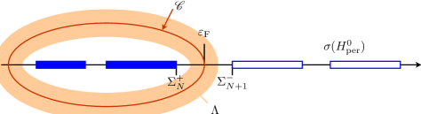
Figure 1. Graphical representation of a contour $\mathscr{C}\subset{\mathbb{C}}$ enclosing $\sigma(H^{0}_{\rm per})\cap(-\infty,\varepsilon_{\rm F}]$ and of the compact set $\Lambda$.

The following result will be useful to expand $Q_{V}$:

Lemma 2.

There exists $\alpha>0$ such that if $V\in L^{2}({\mathbb{R}}^{3})+\mathcal{C}^{\prime}$ is such that

$$\|V\|_{L^{2}+\mathcal{C}^{\prime}}<\alpha,$$

then

(41) $$\sigma\left(H^{0}_{\rm per}+V\right)\cap\Lambda=\emptyset.$$

Moreover $\varepsilon_{\rm F}\notin\sigma\left(H^{0}_{\rm per}+V\right)$, $Q_{V}\in\mathcal{Q}$ and ${\rm Tr}_{0}(Q_{V})=0$.

Besides, there exists an orthonormal basis $(\varphi_{i}^{-})_{i\geq 1}$ of the occupied space ${\mathcal{H}}_{-}=\mbox{Ran}(\gamma^{0}_{\rm per})$ and an orthonormal basis $(\varphi_{i}^{+})_{i\geq 1}$ of the occupied space ${\mathcal{H}}_{+}=\mbox{Ker}(\gamma^{0}_{\rm per})$ such that in the orthonormal basis $((\varphi_{i}^{-}),(\varphi_{i}^{+}))$ of $L^{2}({\mathbb{R}}^{3})={\mathcal{H}}_{-}\widehat{\oplus}{\mathcal{H}}_{+}$,

(42) $$Q_{V}=\left(\begin{array}[]{c||c}\mbox{diag}(-a_{1},-a_{2},\cdots)&\mbox{diag}(b_{1},b_{2},\cdots)\\ \hline\cr\hline\cr\mbox{diag}(b_{1},b_{2},\cdots)&\mbox{diag}(a_{1},a_{2},\cdots)\\ \end{array}\right)$$

with

$$0\leq a_{i}<1,\quad\sum_{i=1}^{+\infty}a_{i}<\infty,\quad b_{i}=\sqrt{a_{i}(1-a_{i})}.$$

The meaning of (41) is the following. As mentioned above, any $V\in L^{2}({\mathbb{R}}^{3})+\mathcal{C}^{\prime}$ defines a compact perturbation of $H^{0}_{\rm per}$; hence the essential spectrum of the Hamiltonian remains unchanged:

$$\sigma_{\rm ess}\left(H^{0}_{\rm per}+V\right)=\sigma_{\rm ess}\left(H^{0}_{\rm per}\right).$$

This in particular means that only eigenvalues of finite multiplicity may appear in the gap $(\Sigma_{N}^{+},\Sigma_{N+1}^{-})$, and they can only accumulate at $\Sigma_{N}^{+}$ or $\Sigma_{N+1}^{-}$. For $V$ small enough in $L^{2}+\mathcal{C}^{\prime}$, these eigenvalues will be localized at the edges of the gap, i.e. in a vicinity of $\Sigma_{N}^{+}$ and $\Sigma_{N+1}^{-}$. It can be seen that the charge ${\rm Tr}_{0}(Q_{tV})$ jumps as $t$ is increased when an eigenvalue crosses the curve $\mathscr{C}$ and that it is a constant integer when this does not happen. By continuity, we deduce that ${\rm Tr}_{0}(Q_{V})=0$: for $V$ small enough, no electron-hole pair is created from the Fermi sea.

The representation (42) of $Q_{V}$ was proved in [11] and it can be interpreted in terms of Bogoliubov states. Each $2\times 2$ submatrix $\left(\begin{array}[]{cc}-a_{i}&b_{i}\\ b_{i}&a_{i}\end{array}\right)$ can be seen as a virtual electron-hole pair. A real electron-hole pair would be observed for $a_{i}=1$. It is easy to see that the eigenvalues of $Q_{V}$ (including multiplicities) are $(-a_{i}^{\frac{1}{2}},a_{i}^{\frac{1}{2}})_{i\geq 1}$. Thus a necessary and sufficient condition for $Q_{V}$ being trace class reads $\sum a_{i}^{\frac{1}{2}}<\infty$.

We now provide the

Proof of Lemma 2.

Let $C\in{\mathbb{R}}_{+}$ be such that for all $z\in\Lambda$, $\|B(z)\|\leq C$ (see the first statement of Lemma 1). For all $z\in\Lambda$,

$$z-H^{0}_{\rm per}-V=(z-H^{0}_{\rm per})(1-B(z)(1-\Delta)^{-1}V).$$

As $L^{2}({\mathbb{R}}^{3})+\mathcal{C}^{\prime}\subset L^{2}({\mathbb{R}}^{3})+L^{6}({\mathbb{R}}^{3})$, it follows from the Kato-Seiler-Simon inequality (39) that there exists a constant $C^{\prime}$ such that

$$\forall V\in L^{2}({\mathbb{R}}^{3})+\mathcal{C}^{\prime},\quad\|(1-\Delta)^{-1}V\|\leq C^{\prime}\|V\|_{L^{2}+\mathcal{C}^{\prime}}.$$

If $\|V\|_{L^{2}+\mathcal{C}^{\prime}}<(CC^{\prime})^{-1}$, $\sigma(H^{0}_{\rm per}+V)\cap\Lambda=\emptyset$. As $V$ defines a compact perturbation of $H^{0}_{\rm per}$, it follows from a standard continuity arguments that for $\|V\|_{L^{2}+\mathcal{C}^{\prime}}<(CC^{\prime})^{-1}$, the set $\sigma(H^{0}_{\rm per}+V)\cap(-\infty,\varepsilon_{\rm F}]$ lays inside the contour $\mathscr{C}$, yielding

$$1_{(-\infty,\varepsilon_{\rm F}]}(H^{0}_{\rm per}+V)=\frac{1}{2i\pi}\oint_{\mathscr{C}}\left(z-H^{0}_{\rm per}-V\right)^{-1}\,dz.$$

Thus,

$$Q_{V}=\frac{1}{2i\pi}\oint_{\mathscr{C}}\left[\left(z-H^{0}_{\rm per}-V\right)^{-1}-\left(z-H^{0}_{\rm per}\right)^{-1}\right]\,dz.$$

Besides, still in the case when $\|V\|_{L^{2}+\mathcal{C}^{\prime}}<(CC^{\prime})^{-1}$,

$$\left(z-H^{0}_{\rm per}-V\right)^{-1}-\left(z-H^{0}_{\rm per}\right)^{-1}=B(z)(1-\Delta)^{-1}V\left(z-H^{0}_{\rm per}-V\right)^{-1},$$

so that

$$\|Q_{V}\|\leq\frac{|\mathscr{C}|}{2\pi}\frac{C^{2}C^{\prime}\|V\|_{L^{2}+\mathcal{C}^{\prime}}}{1-CC^{\prime}\|V\|_{L^{2}+\mathcal{C}^{\prime}}}.$$

We now set $\alpha=((1+(2\pi)^{-1}C|\mathscr{C}|)CC^{\prime})^{-1}$. For all $V\in L^{2}({\mathbb{R}}^{3})+\mathcal{C}^{\prime}$ such that $\|V\|_{L^{2}+\mathcal{C}^{\prime}}<\alpha$, it holds $\sigma(H^{0}_{\rm per}+V)\cap\Lambda=\emptyset$ and $\|Q_{V}\|<1$. We conclude using [10, Lemma 2] and [11, Theorem 5]. ∎

We are now going to expand $Q_{V}$ using the resolvent formula. We already know that

$$\gamma^{0}_{\rm per}=1_{(-\infty,\varepsilon_{\rm F}]}\left(H^{0}_{\rm per}\right)=\frac{1}{2i\pi}\oint_{\mathscr{C}}\left(z-H^{0}_{\rm per}\right)^{-1}\,dz.$$

It now follows from the proof of Lemma 2 that

$$1_{(-\infty,\varepsilon_{\rm F}]}\left(H^{0}_{\rm per}+V\right)=\frac{1}{2i\pi}\oint_{\mathscr{C}}\left(z-H^{0}_{\rm per}-V\right)^{-1}\,dz$$

for all $V\in L^{2}({\mathbb{R}}^{3})+\mathcal{C}^{\prime}$ such that $\|V\|_{L^{2}+\mathcal{C}^{\prime}}<\alpha$, yielding for such $V$’s

$$Q_{V}=\frac{1}{2i\pi}\oint_{\mathscr{C}}\left[\left(z-H^{0}_{\rm per}-V\right)^{-1}-\left(z-H^{0}_{\rm per}\right)^{-1}\right]\,dz.$$

One important result of the present section is the following

Lemma 3 (Resolvent expansion).

Let $V\in L^{2}({\mathbb{R}}^{3})+\mathcal{C}^{\prime}$ such that $\|V\|_{L^{2}+\mathcal{C}^{\prime}}<\alpha$. Then, for all $K\in{\mathbb{N}}\setminus\left\{0\right\}$,

(43) $$Q_{V}=Q_{1,V}+\cdots+Q_{K,V}+\widetilde{Q}_{K+1,V}$$

where

(44) $$Q_{k,V} = \frac{1}{2i\pi}\oint_{\mathscr{C}}\left(z-H^{0}_{\rm per}\right)^{-1}\left[V\left(z-H^{0}_{\rm per}\right)^{-1}\right]^{k}\,dz$$

(45) $$\widetilde{Q}_{k,V} = \frac{1}{2i\pi}\oint_{\mathscr{C}}\left(z-H^{0}_{\rm per}-V\right)^{-1}\left[V\left(z-H^{0}_{\rm per}\right)^{-1}\right]^{k}\,dz$$

For all $k\geq 1$, the operator $Q_{k,V}$ is in $\mathcal{Q}$ and ${\rm Tr}_{0}(Q_{k,V})=0$. For all $k\geq 1$, the operator $\widetilde{Q}_{k,V}$ is in $\mathcal{Q}$ and ${\rm Tr}_{0}(\widetilde{Q}_{k,V})=0$. For all $k\geq 6$, the operators $Q_{k,V}$ and $\widetilde{Q}_{k,V}$ are trace-class and ${\rm Tr}(\widetilde{Q}_{k,V})=0$.

Note that by linearity, the operators $Q_{k,V}$ are well-defined for all $V\in L^{2}({\mathbb{R}}^{3})+\mathcal{C}^{\prime}$, and not only for small $V$’s. It can in fact be shown using the same arguments as in the proof of Lemma 3 that for all $k\geq 1$,

$$(V_{1},\cdots,V_{k})\mapsto\frac{1}{2i\pi}\oint_{\mathscr{C}}\left(z-H^{0}_{\rm per}\right)^{-1}V_{1}\left(z-H^{0}_{\rm per}\right)^{-1}\cdots V_{k}\left(z-H^{0}_{\rm per}\right)^{-1}\,dz$$

is a continuous $k$-linear application from $(L^{2}({\mathbb{R}}^{3})+\mathcal{C}^{\prime})^{k}$ to $\mathcal{Q}$.

Let us now detail the

Proof of Lemma 3.

It follows from the proof of Lemma 2 that each term of the expansion (43) makes sense in the space of bounded operators on $L^{2}({\mathbb{R}}^{3})$. We now have to prove that $Q_{k,V}$ and $\widetilde{Q}_{k,V}$ are in $\mathcal{Q}$ and that their generalized trace is equal to zero. We start by noticing that $Q_{V}$ is indeed a minimizer for the functional

$$E(Q):={\rm Tr}(|H^{0}_{\rm per}-\varepsilon_{\rm F}|(Q^{++}-Q^{--})-\int_{{\mathbb{R}}^{3}}V\rho_{Q}$$

on $\mathcal{K}$. Theorem 1 with the nonlinear term erased then implies that $Q_{V}\in\mathcal{Q}$.

Let us consider $Q_{1,V}$. Decomposing $V$ as $V=V_{2}+V^{\prime}$ with $V_{2}\in L^{2}({\mathbb{R}}^{3})$ and $V^{\prime}\in\mathcal{C}^{\prime}\subset L^{6}({\mathbb{R}}^{3})$, and using the Kato-Seiler-Simon inequality (39) and the first assertion of Lemma 1, $Q_{1,V_{2}}\in\mathfrak{S}_{2}$ and $Q_{1,V^{\prime}}\in\mathfrak{S}_{6}$. Hence, $Q_{1,V}$ is well-defined in $\mathfrak{S}_{6}$. A straightforward application of the residuum formula then shows that $Q_{1,V}^{++}=Q_{1,V}^{--}=0$. As

$$Q_{1,V^{\prime}}^{-+} = \frac{1}{2i\pi}\oint_{\mathscr{C}}\gamma^{0}_{\rm per}(z-H^{0}_{\rm per})^{-1}V^{\prime}(z-H^{0}_{\rm per})^{-1}(\gamma^{0}_{\rm per})^{\perp}dz$$

$$= \frac{1}{2i\pi}\oint_{\mathscr{C}}\gamma^{0}_{\rm per}(z-H^{0}_{\rm per})^{-1}[\gamma^{0}_{\rm per},V^{\prime}](z-H^{0}_{\rm per})^{-1}(\gamma^{0}_{\rm per})^{\perp}dz,$$

we can make use of Lemma 1 to conclude that $Q_{1,V^{\prime}}^{-+}\in\mathfrak{S}_{2}$. Obviously, the same holds true for $Q_{1,V^{\prime}}^{+-}$, so that $Q_{1,V^{\prime}}$, and henceforth $Q_{1,V}$, are in $\mathfrak{S}_{2}$. As $|\nabla|(z-H^{0}_{\rm per})^{-1}$ is a bounded operator, uniformly in $z\in\mathscr{C}$, it is easy to check that $|\nabla|Q_{1,V_{2}}$ and $|\nabla|Q_{1,V^{\prime}}$ both are Hilbert-Schmidt operators. Finally, $|\nabla|Q_{1,V}\in\mathfrak{S}_{2}$ and therefore $Q_{1,V}\in\mathcal{Q}$. As $Q_{1,V}^{++}=Q_{1,V}^{--}=0$, we obviously get ${\rm Tr}_{0}(Q_{1,V})=0$.

Let us now consider $Q_{k,V}$ for $k\geq 2$. The potential $V$ being in $L^{2}({\mathbb{R}}^{3})+L^{6}({\mathbb{R}}^{3})$, we have

• $Q_{2,V}\in\mathfrak{S}_{3}$ and $|\nabla|Q_{2,V}\in\mathfrak{S}_{3}$;

• $Q_{k,V}\in\mathfrak{S}_{2}$ and $|\nabla|Q_{k,V}\in\mathfrak{S}_{2}$ for all $k\geq 3$.

As usual [10, 3], the next step consists in introducing $\gamma^{0}_{\rm per}+(\gamma^{0}_{\rm per})^{\perp}=1$ in (44) in places where $(H^{0}_{\rm per}-z)^{-1}$ appears, and in expanding everything. We will use the notation

$$Q_{2,V}^{--+}:=-\frac{1}{2i\pi}\oint_{\mathscr{C}}\frac{\gamma^{0}_{\rm per}}{H^{0}_{\rm per}-z}V\frac{\gamma^{0}_{\rm per}}{H^{0}_{\rm per}-z}V\frac{(\gamma^{0}_{\rm per})^{\perp}}{H^{0}_{\rm per}-z}dz,$$

and similar definitions for all the other terms. A simple application of the residuum formula tells us that $Q_{2,V}^{+++}=Q_{2,V}^{---}=0$. Therefore, $Q_{2,V}^{--}=Q_{2,V}^{-+-}$ and $Q_{2,V}^{++}=Q_{2,V}^{+-+}$. Now we remark that the terms $Q_{2,V}^{-+-}$ and $Q_{2,V}^{+-+}$ involve two terms of the form $\gamma^{0}_{\rm per}V(\gamma^{0}_{\rm per})^{\perp}=[\gamma^{0}_{\rm per},V](\gamma^{0}_{\rm per})^{\perp}$ (or its adjoint) in their formula. Using Lemma 1, we obtain that $Q_{2,V}^{--}$, $Q_{2,V}^{++}$, $|\nabla|Q_{2,V}^{--}|\nabla|$ and $|\nabla|Q_{2,V}^{++}|\nabla|$ are trace-class operators. Likewise, $Q_{k,V}^{--}$, $Q_{k,V}^{++}$, $|\nabla|Q_{k,V}^{--}|\nabla|$ and $|\nabla|Q_{k,V}^{++}|\nabla|$ are trace-class operators. Lastly, $Q_{2,V}^{-+}=Q_{2,V}^{--+}+Q_{2,V}^{-++}$, both operators of the right-hand side involving one term of the form $\gamma^{0}_{\rm per}V(\gamma^{0}_{\rm per})^{\perp}=[\gamma^{0}_{\rm per},V](\gamma^{0}_{\rm per})^{\perp}$. Consequently $Q_{2,V}^{-+}$ and $|\nabla|Q_{2,V}^{-+}$ are Hilbert-Schmidt. Repeating the same argument for $Q_{2,V}^{+-}$, we obtain that $Q_{2,V}$ and $|\nabla|Q_{2,V}$ are Hilbert-Schmidt. Therefore, all the operators $Q_{k,V}$ are in $\mathcal{Q}$. As $Q_{V}$ also is in $\mathcal{Q}$, $\widetilde{Q}_{k,V}\in\mathcal{Q}$ for all $k\geq 3$. It also follows from the first assertion of Lemma 1 and the Kato-Seiler-Simon inequality that $\widetilde{Q}_{k,V}$ is trace-class for $k\geq 6$.

Using (38) and the Kato-Seiler-Simon inequality (39), we then easily obtain that for all $k\geq 1$, there exists a constant $C_{k}\in{\mathbb{R}}_{+}$ such that

$$\forall V\in L^{2}({\mathbb{R}}^{3})+\mathcal{C}^{\prime},\quad\|Q_{k,V}\|_{\mathcal{Q}}\leq C_{k}\|V\|_{L^{2}+\mathcal{C}^{\prime}}^{k}$$

and that for all $k\geq 2$, there exists a constant $\widetilde{C}_{k}\in{\mathbb{R}}_{+}$ such that

$$\forall V\in L^{2}({\mathbb{R}}^{3})+\mathcal{C}^{\prime}\mbox{ s.t. }\|V\|_{L^{2}+\mathcal{C}^{\prime}}<\alpha,\quad\|\widetilde{Q}_{k,V}\|_{\mathcal{Q}}\leq\widetilde{C}_{k}\|V\|_{L^{2}+\mathcal{C}^{\prime}}^{k}.$$

Let $V\in L^{2}({\mathbb{R}}^{3})+\mathcal{C}^{\prime}$ such that $\|V\|_{L^{2}+\mathcal{C}^{\prime}}<\alpha$. For all $t\in[0,1]$, $\|tV\|_{L^{2}+\mathcal{C}^{\prime}}<\alpha$ and

$$Q_{tV}=Q_{1,tV}+\cdots+Q_{K,tV}+\widetilde{Q}_{K,tV}=tQ_{1,V}+\cdots+t^{K}Q_{K,tV}+\widetilde{Q}_{K+1,tV}.$$

As we know that ${\rm Tr}_{0}(Q_{tV})=0$, we obtain that for all $t\in[0,1]$,

$$0=t{\rm Tr}_{0}(Q_{1,V})+\cdots+t^{K}{\rm Tr}_{0}(Q_{K,tV})+{\rm Tr}_{0}(\widetilde{Q}_{K+1,tV})$$

with $|{\rm Tr}_{0}(\widetilde{Q}_{K+1,tV})|\leq\|\widetilde{Q}_{K+1,tV}\|_{\mathcal{Q}}\leq\widetilde{C}_{K+1}t^{K+1}\|V\|_{L^{2}+\mathcal{C}^{\prime}}^{K+1}$. Hence, ${\rm Tr}_{0}(Q_{k,V})=0$ for all $k\geq 1$ and ${\rm Tr}_{0}(\widetilde{Q}_{k,V})=0$ for all $k\geq 2$. ∎

6.4. Proof of Proposition 1

Let $V\in L^{2}({\mathbb{R}}^{3})+\mathcal{C}^{\prime}$. We already know from Lemma 3 that $Q_{1,V}\in\mathcal{Q}$ and that ${\rm Tr}_{0}(Q_{1,V})=0$. Decomposing $V$ as $V=V_{2}+V^{\prime}$ with $V_{2}\in L^{2}({\mathbb{R}}^{3})$ and $V^{\prime}\in\mathcal{C}^{\prime}$, and proceeding as in Section 6.3, we obtain

$$\|Q_{1,V_{2}}\|_{\mathcal{Q}}\leq C\|V_{2}\|_{L^{2}},$$

$$\|Q_{1,V^{\prime}}\|_{\mathcal{Q}}\leq C\|V^{\prime}\|_{\mathcal{C}^{\prime}}.$$

We infer that $\chi_{0}$ is a continuous linear application from from $L^{2}({\mathbb{R}}^{3})+\mathcal{C}^{\prime}$ to $L^{2}({\mathbb{R}}^{3})\cap\mathcal{C}$.

Let us now examine the case when $V\in L^{1}({\mathbb{R}}^{3})$. Using again the Kato-Seiler-Simon inequality and the first assertion of Lemma 1, we obtain $Q_{1,V}\in\mathfrak{S}_{1}$ and

$$\|Q_{1,V}\|_{\mathfrak{S}_{1}}\leq C\|V\|_{L^{1}}.$$

Consequently, $\chi_{0}$ defines a continuous linear application from $L^{1}({\mathbb{R}}^{3})$ to $L^{1}({\mathbb{R}}^{3})$. As from the residuum formula, $Q_{1,V}^{++}=Q_{1,V}^{--}=0$, we get ${\rm Tr}(Q_{1,V})=0$. ∎

6.5. Proof of Proposition 3

As $\rho\in L^{1}({\mathbb{R}}^{3})\subset v_{\rm c}^{-1}(L^{2}({\mathbb{R}}^{3}))+\mathcal{C}$, we have $\mathcal{L}(\rho)\in L^{2}({\mathbb{R}}^{3})\cap\mathcal{C}$. The operator $\mathcal{L}$ can be explicitely calculated in Bloch transform. We start from the Bloch-Floquet decomposition of $H^{0}_{\rm per}$: for $f\in H^{2}({\mathbb{R}}^{3})$,

$$(H^{0}_{\rm per}f)(x)=\fint_{\Gamma^{\ast}}((H^{0}_{\rm per})_{q}f_{q})\,e^{iq\cdot x}\,dq$$

where (see Eq. (12))

$$(H^{0}_{\rm per})_{q}=\sum_{n=1}^{+\infty}\varepsilon_{n,q}|u_{n,q}\rangle\langle u_{n,q}|.$$

Note that by time-reversal symmetry,

$$u_{n,-q}=\overline{u_{n,q}},\qquad\varepsilon_{n,-q}=\varepsilon_{n,q}.$$

Denoting by $V=v_{\rm c}(\rho)$, we can write the Bloch matrix of the operator $Q_{1,V}$ as:

(46) $$[Q_{1,V}]_{qq^{\prime}}=\frac{1}{2i\pi}\oint_{\mathscr{C}}(z-(H^{0}_{\rm per})_{q})^{-1}V_{q-q^{\prime}}(z-(H^{0}_{\rm per})_{q^{\prime}})^{-1}\,dz.$$

Inserting the spectral decomposition of $H^{0}_{\rm per}$ in (46), we obtain

(47) $$[Q_{1,V}]_{qq^{\prime}}=-\sum_{n=1}^{N}\sum_{n^{\prime}=N+1}^{+\infty}\bigg{(}\frac{1}{\varepsilon_{n^{\prime},q^{\prime}}-\varepsilon_{n,q}}{\left\langle u_{n,q},V_{q-q^{\prime}}u_{n^{\prime},q^{\prime}}\right\rangle}_{L^{2}_{\rm per}(\Gamma)}|u_{n,q}\rangle\langle u_{n^{\prime},q^{\prime}}|\\ +\frac{1}{\varepsilon_{n^{\prime},q}-\varepsilon_{n,q^{\prime}}}{\left\langle u_{n^{\prime},q},V_{q-q^{\prime}}u_{n,q^{\prime}}\right\rangle}_{L^{2}_{\rm per}(\Gamma)}|u_{n^{\prime},q}\rangle\langle u_{n,q^{\prime}}|\bigg{)}.$$

Remark 2.

In the following we will write series of the form (47) and we will invert sums and integrals without giving any justification. To see that such a series is absolutely convergent, one can use the fact that there exists $a$ and $b$ in ${\mathbb{R}}_{+}$ such that for all $n\geq 1$ and $q\in\Gamma^{\ast}$,

$$\varepsilon_{n,q}\geq an^{2/3}-b.$$

This bound is easily obtained by comparison with the eigenvalues of the periodic Laplacian. It follows that there exists $C\in{\mathbb{R}}_{+}$ such that

$$|{\left\langle u_{n,q},V_{q-q^{\prime}}u_{n^{\prime},q^{\prime}}\right\rangle}_{L^{2}_{\rm per}(\Gamma)}|\leq\frac{C}{(n^{\prime})^{2/3}}$$

for all $1\leq n\leq N$, all $n^{\prime}\geq N+1$ and all $q,q^{\prime}\in\Gamma^{\ast}$.

If an operator $A\in\mathcal{Q}$ has a Bloch matrix $A_{qq^{\prime}}$, then we have

(48) $$(\rho_{A})_{q}(x)=\fint_{\Gamma^{\ast}}A_{q^{\prime},q^{\prime}-q}(x,x)\,dq^{\prime}.$$

This formula is obtained by writing, for any real-valued function $f\in L^{2}({\mathbb{R}}^{3})$,

$$\fint_{\Gamma^{\ast}}{\left\langle(\rho_{A})_{q},f_{q}\right\rangle}_{L^{2}_{\rm per}(\Gamma)}\,dq = \int_{{\mathbb{R}}^{3}}\rho_{A}(x)f(x)\,dx$$

$$= {\rm Tr}(Af)=\fint_{\Gamma^{\ast}}{\rm Tr}_{{L^{2}_{\rm per}(\Gamma)}}\big{(}(Af)_{q^{\prime},q^{\prime}}\big{)}\,dq^{\prime}$$

$$= \fint_{\Gamma^{\ast}}dq^{\prime}\fint_{\Gamma^{\ast}}dq^{\prime\prime}\;{\rm Tr}_{L^{2}_{\rm per}(\Gamma)}\big{(}A_{q^{\prime},q^{\prime\prime}}f_{q^{\prime\prime}-q^{\prime}}\big{)}$$

$$= \int_{\Gamma}dx\fint_{\Gamma^{\ast}}dq^{\prime}\fint_{\Gamma^{\ast}}dq\;\overline{A_{q^{\prime}+q,q^{\prime}}(x,x)}{f_{q}(x)}.$$

We deduce that

(49) $$[\mathcal{L}(\rho)]_{q}(x)=\fint_{\Gamma^{\ast}}dq^{\prime}\sum_{n=1}^{N}\sum_{n^{\prime}=N+1}^{+\infty}\\ \bigg{(}\frac{1}{\varepsilon_{n^{\prime},q^{\prime}-q}-\varepsilon_{n,q^{\prime}}}{\left\langle u_{n,q^{\prime}},(\rho\star|\cdot|^{-1})_{q}u_{n^{\prime},q^{\prime}-q}\right\rangle}_{L^{2}_{\rm per}(\Gamma)}u_{n,q^{\prime}}(x)\overline{u_{n^{\prime},q^{\prime}-q}(x)}\\ +\frac{1}{\varepsilon_{n^{\prime},q^{\prime}}-\varepsilon_{n,q^{\prime}-q}}{\left\langle u_{n^{\prime},q^{\prime}},(\rho\star|\cdot|^{-1})_{q}u_{n,q^{\prime}-q}\right\rangle}_{L^{2}_{\rm per}(\Gamma)}u_{n^{\prime},q^{\prime}}(x)\overline{u_{n,q^{\prime}-q}}(x)\bigg{)}.$$

The next step consists in decomposing the operator $\mathcal{L}$ as the sum of a singular part and a regular part, corresponding respectively to the low and high Fourier modes of the Coulombic interaction kernel $|\cdot|^{-1}$. More precisely, we choose some smooth function $\xi$ which equals $1$ in a small neighborhood $B(0,\delta)$ of 0 and 0 outside the ball $B(0,2\delta)$, with $\delta>0$ such that $B(0,2\delta)\subset\Gamma^{\ast}$. Then we define

$$\mathcal{L}_{s}(\rho):=\mathcal{L}\left(\mathcal{F}^{-1}\xi\widehat{\rho}\right),\qquad\mathcal{L}_{r}(\rho):=\mathcal{L}\left(\mathcal{F}^{-1}(1-\xi)\widehat{\rho}\right)$$

where $\mathcal{F}^{-1}$ is the inverse Fourier tranform. Similarly we define

$$v_{s}:=\sqrt{\frac{2}{\pi}}\mathcal{F}^{-1}(\xi(\cdot)|\cdot|^{-2}),\qquad v_{r}:=\sqrt{\frac{2}{\pi}}\mathcal{F}^{-1}((1-\xi(\cdot))|\cdot|^{-2})$$

and note that $v_{r}\in L^{1}({\mathbb{R}}^{3})$. This being said, we have by the Kato-Seiler-Simon inequality (39) that

$$Q_{1}^{r}:=\frac{1}{2i\pi}\oint_{\mathscr{C}}(z-H^{0}_{\rm per})^{-1}(\rho\star v_{r})(z-H^{0}_{\rm per})^{-1}dz\in\mathfrak{S}_{1},$$

hence $\mathcal{L}_{r}(\rho)\in L^{1}({\mathbb{R}}^{3})$ and $\int_{{\mathbb{R}}^{3}}\mathcal{L}_{r}(\rho)=0$ by Proposition 1. Consequently, $\widehat{\mathcal{L}_{r}(\rho)}\in C^{0}({\mathbb{R}}^{3})$ and $\widehat{\mathcal{L}_{r}(\rho)}(0)=0$.

Let us now deal with the singular part of $\mathcal{L}(\rho)$. Using the definition (13) of the Bloch-Floquet transform, we obtain that

$$(|\cdot|^{-1})_{q}(x)=\frac{4\pi}{|\Gamma|}\sum_{K\in\mathcal{R}^{\ast}}\frac{e^{iK\cdot x}}{|q+K|^{2}}$$

and that for almost all $q\in\Gamma^{\ast}$,

$$\left(\mathcal{F}^{-1}(\xi\widehat{\rho})\right)_{q}(x)=\frac{(2\pi)^{\frac{3}{2}}}{|\Gamma|}\widehat{\rho}(q)\xi(q).$$

This implies that for almost all $q\in\Gamma^{\ast}$,

(50) $$(\rho\star v_{s})_{q}(x)=4\pi\frac{(2\pi)^{\frac{3}{2}}}{|\Gamma|}\frac{\xi(q)\widehat{\rho}(q)}{|q|^{2}}.$$

Therefore we get for almost all $q\in\Gamma^{\ast}$,

(51) $$\mathcal{L}_{s}(\rho)_{q}(x)=(2\pi)^{\frac{3}{2}}\frac{B_{q}(x)}{|q|^{2}}\widehat{\rho}(q)$$

where

(52) $$B_{q}(x):=\frac{4\pi}{|\Gamma|}\xi(q)\fint_{\Gamma^{\ast}}d{q^{\prime}}\sum_{n=1}^{N}\sum_{n^{\prime}=N+1}^{+\infty}\\ \bigg{(}\frac{1}{\varepsilon_{n^{\prime},{q^{\prime}}-q}-\varepsilon_{n,{q^{\prime}}}}{\left\langle u_{n,{q^{\prime}}},u_{n^{\prime},{q^{\prime}}-q}\right\rangle}_{L^{2}_{\rm per}(\Gamma)}u_{n,{q^{\prime}}}(x)\overline{u_{n^{\prime},{q^{\prime}}-q}(x)}\\ +\frac{1}{\varepsilon_{n^{\prime},{q^{\prime}}}-\varepsilon_{n,{q^{\prime}}-q}}{\left\langle u_{n^{\prime},{q^{\prime}}},u_{n,{q^{\prime}}-q}\right\rangle}_{L^{2}_{\rm per}(\Gamma)}u_{n^{\prime},{q^{\prime}}}(x)\overline{u_{n,{q^{\prime}}-q}(x)}\bigg{)}.$$

It follows that almost everywhere in $\Gamma^{\ast}$,

$$\widehat{\mathcal{L}_{s}(\rho)}(q) = (2\pi)^{-\frac{3}{2}}\int_{\Gamma}\mathcal{L}_{s}(\rho)_{q}(x)dx$$

$$= \frac{{\mathcal{B}}(q)}{|q|^{2}}\widehat{\rho}(q)$$

where

(53) $${\mathcal{B}}(q)=\frac{8\pi}{|\Gamma|}\xi(q)\sum_{n=1}^{N}\sum_{n^{\prime}=N+1}^{+\infty}\fint_{\Gamma^{\ast}}d{q^{\prime}}\frac{\left|{\left\langle u_{n,{q^{\prime}}},u_{n^{\prime},{q^{\prime}}-q}\right\rangle}_{L^{2}_{\rm per}(\Gamma)}\right|^{2}}{\varepsilon_{n^{\prime},{q^{\prime}-q}}-\varepsilon_{n,{q^{\prime}}}}.$$

We now remark that the above formula may be written

$${\mathcal{B}}(q)=-\frac{8\pi}{|\Gamma|}\xi(q){\rm Tr}_{L^{2}_{\rm per}}\left[\oint_{\mathscr{C}}dz\fint_{\Gamma^{\ast}}d{q^{\prime}}\frac{\left(\gamma^{0}_{\rm per}\right)_{q^{\prime}}}{z-(H^{0}_{\rm per})_{q^{\prime}}}\;\frac{\left(\gamma^{0}_{\rm per}\right)_{q^{\prime}-q}^{\perp}}{z-(H^{0}_{\rm per})_{q^{\prime}-q}}\right].$$

We recall [17] that $q\mapsto\left(\gamma^{0}_{\rm per}\right)_{q}$ is a smooth periodic function and that $\left(\gamma^{0}_{\rm per}\right)_{q}$ is for all $q$ a rank-$N$ orthogonal projector. It is then easy to deduce that $q\mapsto\mathcal{B}(q)$ is a continuous periodic function on ${\mathbb{R}}^{3}$. Consequently, $\widehat{\mathcal{L}_{s}(\rho)}$ and therefore $\widehat{\mathcal{L}(\rho)}$ are continuous on $\Gamma^{\ast}\setminus\left\{0\right\}$. Using similar arguments, one obtains that $\widetilde{\mathcal{L}(\rho)}$ is continuous on ${\mathbb{R}}^{3}\setminus\mathcal{R}^{\ast}$. In order to study the limit of $\widehat{\mathcal{L}_{s}(\rho)}(q)$ when $q$ goes to zero, we use the relation

(54) $$\left[\left(\varepsilon_{n^{\prime},q^{\prime}-q}-\frac{|q^{\prime}-q|^{2}}{2}\right)-\left(\varepsilon_{n,q^{\prime}}-\frac{|q^{\prime}|^{2}}{2}\right)\right]\langle u_{n,q^{\prime}},u_{n^{\prime}q^{\prime}-q}\rangle_{L^{2}_{\rm per}(\Gamma)}\\ =-\langle iq\cdot\nabla u_{n,q^{\prime}},u_{n^{\prime},q^{\prime}-q}\rangle_{L^{2}_{\rm per}(\Gamma)}$$

to rewrite $\widehat{\mathcal{L}_{s}(\rho)}(\eta\sigma)$ for $\sigma\in S^{2}$ and $\eta>0$ small enough as

$$\widehat{\mathcal{L}_{s}(\rho)}(\eta\sigma)=L_{\eta}(\sigma)\widehat{\rho}(\eta\sigma)$$

where

$$L_{\eta}(\sigma)=\frac{8\pi}{|\Gamma|}\sum_{n=1}^{N}\sum_{n^{\prime}=N+1}^{+\infty}\fint_{\Gamma^{\ast}}d{q^{\prime}}\frac{\left|\langle\sigma\cdot\nabla u_{n,q^{\prime}},u_{n^{\prime},q^{\prime}-\eta\sigma}\rangle_{L^{2}_{\rm per}(\Gamma)}\right|^{2}}{(\varepsilon_{n^{\prime},{q^{\prime}-\eta\sigma}}-\varepsilon_{n,{q^{\prime}}})(\varepsilon_{n^{\prime},{q^{\prime}-\eta\sigma}}-\varepsilon_{n,{q^{\prime}}}+\eta q^{\prime}\cdot\sigma-\frac{\eta^{2}}{2})^{2}}$$

(recall that $\xi\equiv 1$ in the vicinity of $0$). Again the above formula may be rewritten as

$$L_{\eta}(\sigma)=\frac{8\pi}{|\Gamma|}\sum_{n=1}^{N}\fint_{\Gamma^{\ast}}d{q^{\prime}}\times\\ {\left\langle\frac{\left(\gamma^{0}_{\rm per}\right)^{\perp}_{q^{\prime}-\eta\sigma}}{\left((H^{0}_{\rm per})_{q^{\prime}-\eta\sigma}-\varepsilon_{n,{q^{\prime}}}\right)\left((H^{0}_{\rm per})_{q^{\prime}-\eta\sigma}-\varepsilon_{n,{q^{\prime}}}+\eta q^{\prime}\cdot\sigma-\frac{\eta^{2}}{2}\right)^{2}}\sigma\cdot\nabla u_{n,q^{\prime}},\sigma\cdot\nabla u_{n,q^{\prime}}\right\rangle}_{L^{2}_{\rm per}(\Gamma)}$$

which shows that when $\eta$ goes to zero, $L_{\eta}(\sigma)$ converges to $\sigma^{T}L\sigma$ while $\widehat{\rho}(\eta\sigma)$ converges to $\widehat{\rho}(0)$.

We now turn to the proof that $L_{0}>0$. We note first that

$$L_{0}=\frac{1}{3}\frac{8\pi}{|\Gamma|}\sum_{n=1}^{N}\sum_{n^{\prime}=N+1}^{+\infty}\fint_{\Gamma^{\ast}}d{q^{\prime}}\frac{\left|\langle\nabla u_{n,q^{\prime}},u_{n^{\prime},q^{\prime}}\rangle_{L^{2}_{\rm per}(\Gamma)}\right|^{2}}{(\varepsilon_{n^{\prime},{q^{\prime}}}-\varepsilon_{n,{q^{\prime}}})^{3}}$$

hence $L_{0}=0$ would imply $\langle\nabla u_{n,q},u_{n^{\prime},q}\rangle_{L^{2}_{\rm per}(\Gamma)}=0$ for all $q\in\Gamma^{\ast}$, all $n\leq N$ and all $n^{\prime}\geq N+1$. Hence for $i=1,2,3$, $\partial_{x_{i}}$ would stabilize the space $X_{q}$ spanned by $(u_{1,q},...,u_{N,q})$ for any $q$. Next we differentiate the eigenvalue equation for $u_{n,q}$ and get

$$\left(-\frac{\Delta}{2}-iq\cdot\nabla+\frac{|q|^{2}}{2}+V_{\rm per}-\varepsilon_{n,q}\right)\partial_{x_{i}}u_{n,q}+(\partial_{x_{i}}V_{\rm per})u_{n,q}=0.$$

From this we deduce that $(\partial_{x_{i}}V_{\rm per})$ would also stabilize $X_{q}$. This means that we would have

$$\forall x\in\Gamma,\qquad(\partial_{x_{i}}V_{\rm per})(x)\left(\begin{array}[]{c}u_{1,q}(x)\\ \vdots\\ u_{N,q}(x)\\ \end{array}\right)=A_{q}\left(\begin{array}[]{c}u_{1,q}(x)\\ \vdots\\ u_{N,q}(x)\\ \end{array}\right)$$

for some matrix $A_{q}$ depending only on $q$. As $u_{1,0}(x)>0$ for all $x$ (it is the first eigenfunction of a Schrödinger operator), we deduce that $(\partial_{x_{i}}V_{\rm per})(x)$ would be for any $x\in\Gamma$ an eigenvalue of $A_{0}$. By continuity and periodicity we infer that $V_{\rm per}$ would be constant. This is in contradiction with the assumption that the host crystal is an insulator or a semiconductor. ∎

6.6. Proof of Proposition 2

The proof of Proposition 1 shows that $\mathcal{L}$ defines a bounded linear operator on $\mathcal{C}$. Besides, for all $\rho_{1}$ and $\rho_{2}$ in $\mathcal{C}$,

$$\langle\mathcal{L}(\rho_{1}),\rho_{2}\rangle = \int_{{\mathbb{R}}^{3}}[\mathcal{L}(\rho_{1})](x)\,[v_{\rm c}(\rho_{2})](x)\,dx$$

$$= -\frac{1}{2i\pi}\oint_{\mathscr{C}}{\rm Tr}\left((z-H^{0}_{\rm per})^{-1}v_{\rm c}(\rho_{1})(z-H^{0}_{\rm per})^{-1}v_{\rm c}(\rho_{2})\right)\,dz$$

$$= \langle\mathcal{L}(\rho_{2}),\rho_{1}\rangle=\langle\rho_{1},\mathcal{L}(\rho_{2})\rangle.$$

Therefore, $\mathcal{L}$ is self-adjoint on $\mathcal{C}$. Lastly, denoting by $V=v_{\rm c}(\rho)$, we have for all $\rho\in\mathcal{C}$,

$${\left\langle\mathcal{L}(\rho),\rho\right\rangle}_{\mathcal{C}} =\int_{{\mathbb{R}}^{3}}\mathcal{L}(\rho)(x)V(x)\,dx=\fint_{\Gamma^{\ast}}\int_{\Gamma}\overline{\mathcal{L}(\rho)_{q}(x)}\,V_{q}(x)\,dx\,dq$$

$$=\sum_{n=1}^{N}\sum_{n^{\prime}=N+1}^{+\infty}\fint_{\Gamma^{\ast}}dq\fint_{\Gamma^{\ast}}d{q^{\prime}}\Bigg{(}\frac{\big{|}{\left\langle u_{n,{q^{\prime}}},V_{q}u_{n^{\prime},{q^{\prime}}-q}\right\rangle}_{L^{2}_{\rm per}(\Gamma)}\big{|}^{2}}{\varepsilon_{n^{\prime},{q^{\prime}}-q}-\varepsilon_{n,{q^{\prime}}}}$$

$$\qquad\qquad\qquad\qquad\qquad+\frac{\left|{\left\langle u_{n^{\prime},{q^{\prime}}},V_{q}u_{n,{q^{\prime}}-q}\right\rangle}_{L^{2}_{\rm per}(\Gamma)}\right|^{2}}{\varepsilon_{n^{\prime},{q^{\prime}}}-\varepsilon_{n,{q^{\prime}}-q}}\Bigg{)}\geq 0.$$

We conclude that $\mathcal{L}$ is a bounded positive self-adjoint operator on $\mathcal{C}$. Consequently, $1+\mathcal{L}\,:\,\mathcal{C}\rightarrow\mathcal{C}$ is invertible. ∎

6.7. Expanding the density to higher orders

In the previous sections, we have studied the first order density $-\mathcal{L}(\rho)$. For the proof of our Theorem 2 on the reduced-Hartree-Fock model, we need to consider the higher order terms. Each of the operators $Q_{k,V}$ (for $k\geq 1$) and $\widetilde{Q}_{k,V}$ (for $k\geq 2$) defined in Lemma 2 being in $\mathcal{Q}$, the expansion (43) can be rewritten in terms of the associated densities, yielding the following equation in $L^{2}({\mathbb{R}}^{3})\cap\mathcal{C}$:

(55) $$\rho_{Q_{V}}=\rho_{Q_{1,V}}+\cdots+\rho_{Q_{K,V}}+\rho_{\widetilde{Q}_{K+1,V}}.$$

We introduce the quadratic operator $r_{2}$ defined by

$$r_{2}(\rho)=\rho_{Q_{2,v_{\rm c}(\rho)}},$$

which is continuous from $v_{\rm c}^{-1}(L^{2}({\mathbb{R}}^{3}))+\mathcal{C}$ to $L^{2}({\mathbb{R}}^{3})\cap\mathcal{C}$, and the nonlinear map $\widetilde{r}_{3}$ from $v_{\rm c}^{-1}(B_{\alpha})$ to $L^{2}({\mathbb{R}}^{3})\cap\mathcal{C}$ ($B_{\alpha}$ denoting the ball of $L^{2}({\mathbb{R}}^{3})+\mathcal{C}^{\prime}$ of radius $\alpha$), defined by

$$\widetilde{r}_{3}(\rho)=\rho_{\widetilde{Q}_{3,v_{\rm c}(\rho)}}.$$

We obtain

(56) $$r(\rho):=\rho_{Q_{v_{\rm c}(\rho)}}=-\mathcal{L}(\rho)+r_{2}(\rho)+\widetilde{r}_{3}(\rho).$$

The next lemma is concerned with the second and third order terms of the expansion (56). We will assume that $\rho\in L^{1}({\mathbb{R}}^{3})\cap L^{2}({\mathbb{R}}^{3})$. Then $\rho\in L^{\frac{6}{5}}({\mathbb{R}}^{3})\subset\mathcal{C}$, so that $v_{\rm c}(\rho)\in\mathcal{C}^{\prime}$ and $\|v_{\rm c}(\rho)\|_{\mathcal{C}^{\prime}}\leq C\|\rho\|_{L^{1}\cap L^{2}}$, where $C$ is a universal constant. In particular, there exists a constant $\gamma>0$, such that

$$\|\rho\|_{L^{1}\cap L^{2}}\leq\gamma\quad\Rightarrow\quad\|v_{\rm c}(\rho)\|_{L^{2}+\mathcal{C}^{\prime}}\leq\|v_{\rm c}(\rho)\|_{\mathcal{C}^{\prime}}<\alpha.$$

Lemma 4 (Nonlinear terms in the expansion).

Let $\rho\in L^{1}({\mathbb{R}}^{3})\cap L^{2}({\mathbb{R}}^{3})$. Then

1. $Q_{2}(\rho)\in\mathfrak{S}_{p}$ for all $p>1$ and the Fourier transform $\widehat{r_{2}(\rho)}$ of $r_{2}(\rho)$ is continuous on ${\mathbb{R}}^{3}$ and vanishes at $k=0$ ;

2. If in addition, $\|\rho\|_{L^{1}\cap L^{2}}\leq\gamma$, then $\widetilde{Q}_{3}(\rho)\in\mathfrak{S}_{1}$, $\widetilde{r}_{3}(\rho)\in L^{1}({\mathbb{R}}^{3})$ and

   $${\rm Tr}(\widetilde{Q}_{3}(\rho))=\int_{{\mathbb{R}}^{3}}\widetilde{r}_{3}(\rho)=0.$$

Proof of Lemma 4.

As $\rho\in L^{1}({\mathbb{R}}^{3})\cap L^{2}({\mathbb{R}}^{3})$, we deduce from Young inequality that $V=\rho\star|\cdot|^{-1}$ is in $L^{p}({\mathbb{R}}^{3})$ for $3<p<\infty$ and that $\nabla V$ is in $(L^{q}({\mathbb{R}}^{3}))^{3}$ for all $\frac{3}{2}<q<6$. Therefore,

$$\left\|[\gamma^{0}_{\rm per},V]\right\|_{\mathfrak{S}_{q}}\leq C_{q}\|\nabla V\|_{L^{q}}$$

for all $\frac{3}{2}<q<6$, by Lemma 1. Arguing as in the proof of Lemma 3, we obtain that $Q_{2,V}\in\mathfrak{S}_{p}$ for all $p>1$.

We now concentrate on the regularity of $\widehat{r_{2}(\rho)}=\widehat{\rho}_{Q_{2,V}}$ at the origin. Arguing like in the proof of Proposition 3, we only have to study the density associated with the operator

$$R_{2}:=\frac{1}{2i\pi}\oint_{\mathscr{C}}(z-H^{0}_{\rm per})^{-1}\left(\rho\star v_{s}\right)(z-H^{0}_{\rm per})^{-1}\left(\rho\star v_{s}\right)(z-H^{0}_{\rm per})^{-1}dz.$$

We will for simplicity only treat the term $R_{2}^{-++}$, the other ones being similar. Following the proof of Proposition 3, we obtain

(57) $$\widehat{\rho_{R_{2}^{-++}}}(q)=(2\pi)^{-\frac{3}{2}}\sum_{n=1}^{N}\sum_{m\geq N+1}\sum_{m^{\prime}\geq N+1}\fint_{\Gamma^{\ast}}dq^{\prime}\fint_{\Gamma^{\ast}}dr\\ \frac{{\left\langle u_{n,q^{\prime}},(\rho\star v_{s})_{q^{\prime}-r}u_{m,r}\right\rangle}{\left\langle u_{m,r},(\rho\star v_{s})_{r-q^{\prime}+q}u_{m^{\prime},q^{\prime}-q}\right\rangle}{\left\langle u_{m^{\prime},q^{\prime}-q},u_{n,q^{\prime}}\right\rangle}}{(\varepsilon_{n,q^{\prime}}-\varepsilon_{m,r})(\varepsilon_{n,q^{\prime}}-\varepsilon_{m^{\prime},q^{\prime}-q})}.$$

Changing $r\leftarrow r-q^{\prime}$ and using as before (50), we see that for $|q|$ small enough,

(58) $$\widehat{\rho_{R_{2}^{-++}}}(q)=4\sqrt{2\pi}\sum_{n=1}^{N}\sum_{m\geq N+1}\sum_{m^{\prime}\geq N+1}\fint_{\Gamma^{\ast}}dq^{\prime}\fint_{\Gamma^{\ast}}dr\xi(-r)\xi(r+q)\times\\ \times\frac{\widehat{\rho}(-r)\widehat{\rho}(r+q){\left\langle u_{n,q^{\prime}},u_{m,r+q^{\prime}}\right\rangle}{\left\langle u_{m,r+q^{\prime}},u_{m^{\prime},q^{\prime}-q}\right\rangle}{\left\langle u_{m^{\prime},q^{\prime}-q},u_{n,q^{\prime}}\right\rangle}}{|r|^{2}|r+q|^{2}(\varepsilon_{n,q^{\prime}}-\varepsilon_{m,r-q^{\prime}})(\varepsilon_{n,q^{\prime}}-\varepsilon_{m^{\prime},q^{\prime}-q})}.$$

Next, using (54), we obtain

(59) $$|\widehat{\rho_{R_{2}^{-++}}}(q)|\leq C|q|\sum_{n=1}^{N}\sum_{m\geq N+1}\sum_{m^{\prime}\geq N+1}\fint_{\Gamma^{\ast}}dq^{\prime}\fint_{\Gamma^{\ast}}dr\frac{\xi(-r)\xi(r+q)}{|r|\;|r+q|^{2}}\times\\ \times\frac{|\widehat{\rho}(-r)|\;|{\left\langle\nabla u_{n,q^{\prime}},u_{m,r+q^{\prime}}\right\rangle}|}{|\varepsilon_{m,r+q^{\prime}}-\varepsilon_{n,q^{\prime}}-r\cdot(r+2q^{\prime})/2|}\times\\ \times\frac{|\widehat{\rho}(r+q)|\;|{\left\langle u_{m^{\prime},q^{\prime}-q},\nabla u_{n,q^{\prime}}\right\rangle}|}{(\varepsilon_{m,r-q^{\prime}}-\varepsilon_{n,q^{\prime}})(\varepsilon_{m^{\prime},q^{\prime}-q}-\varepsilon_{n,q^{\prime}})|\varepsilon_{n,q^{\prime}}-\varepsilon_{m^{\prime},q^{\prime}-q}+q\cdot(q-2q^{\prime})/2|}.$$

Note that choosing the support of $\xi$ small enough we have

$$|\varepsilon_{m,r+q^{\prime}}-\varepsilon_{n,q^{\prime}}-r\cdot(r+2q^{\prime})/2|\geq c(m^{2/3}+1)$$

uniformly for $r,q^{\prime}\in\Gamma^{\ast}$ and $n=1..N$. Similarly, taking $q$ small enough we get

$$|\varepsilon_{n,q^{\prime}}-\varepsilon_{m^{\prime},q^{\prime}-q}+q\cdot(q-2q^{\prime})/2|\geq c((m^{\prime})^{2/3}+1).$$

Using these estimates and the fact that $\rho\in L^{1}$ we deduce that

$$|\widehat{\rho_{R_{2}^{-++}}}(q)|\leq C|q|\int_{{\mathbb{R}}^{3}}\frac{\xi(-r)}{|r|\;|r+q|^{2}}\,dr\leq C|q|\log\frac{1}{|q|}$$

and the result follows.

To establish that $\widetilde{Q}_{3,V}$ is trace-class, and therefore that $\widetilde{r}_{3}(\rho)$ is integrable, we write

$$\widetilde{Q}_{3,V}=Q_{3,V}+\widetilde{Q}_{4,V}$$

and proceed as above to prove that both operators in the right hand side are trace-class. As ${\rm Tr}_{0}(\widetilde{Q}_{3,V})=0$, we readily conclude that ${\rm Tr}(\widetilde{Q}_{3,V})=\int_{{\mathbb{R}}^{3}}\widetilde{r}_{3}(\rho)=0$. ∎

6.8. Proof of Theorem 2

We now have all the material for proving Theorem 2. The first step is to confirm that if the external potential $\nu\star|\cdot|^{-1}$ is small, so is the effective potential $(\nu-\rho_{\nu,\varepsilon_{\rm F}})\star|\cdot|^{-1}$, hence the results of Section 6.3 can be applied.

Lemma 5.

There exists $\beta>0$ such that if

$$\|\nu\star|\cdot|^{-1}\|_{L^{2}+\mathcal{C}^{\prime}}<\beta,$$

then

$$\|(\nu-\rho_{\nu,\varepsilon_{\rm F}})\star|\cdot|^{-1}\|_{L^{2}+\mathcal{C}^{\prime}}<\alpha$$

where $\alpha$ is the constant used in the formulation of Lemma 2. Consequently, the solution to (18) is unique and satisfies ${\rm Tr}_{0}(Q_{\nu,\varepsilon_{\rm F}})=0$ and

(60) $$Q_{\nu,\varepsilon_{\rm F}} = 1_{(-\infty,\varepsilon_{\rm F}]}\left(H^{0}_{\rm per}+(\rho_{\nu,\varepsilon_{\rm F}}-\nu)\star|\cdot|^{-1}\right)-1_{(-\infty,\varepsilon_{\rm F}]}\left(H^{0}_{\rm per}\right)$$

$$= \frac{1}{2i\pi}\oint_{\mathscr{C}}\left[\left(z-H^{0}_{\rm per}-(\rho_{\nu,\varepsilon_{\rm F}}-\nu)\star|\cdot|^{-1}\right)^{-1}-\left(z-H^{0}_{\rm per}\right)^{-1}\right]\,dz.$$

Proof of Lemma 5.

Let $0<\delta<1$ and $\nu$ such that $\|\nu\star|\cdot|^{-1}\|_{L^{2}+\mathcal{C}^{\prime}}\leq\delta$. This implies that

$$\nu\star|\cdot|^{-1}=V_{2}+\nu^{\prime}\star|\cdot|^{-1}$$

with $V_{2}\in L^{2}({\mathbb{R}}^{3})$, $\nu^{\prime}\in\mathcal{C}$, $\|V_{2}\|_{L^{2}}\leq\delta$ and $\|\nu^{\prime}\|_{\mathcal{C}}\leq\delta$. We then deduce from (40) that

$$0=E_{\nu,\varepsilon_{\rm F}}(0)\geq E_{\nu,\varepsilon_{\rm F}}(Q_{\nu,\varepsilon_{\rm F}})\geq\frac{c_{1}}{2}{\rm Tr}\left((1+|\nabla|^{2})(Q^{++}_{\nu,\varepsilon_{\rm F}}-Q^{--}_{\nu,\varepsilon_{\rm F}})\right)-C^{\prime}\delta-\frac{\delta^{2}}{2}.$$

It follows that there exists a constant $c\in{\mathbb{R}}_{+}$ independent of $\delta$ and $\nu$ such that

$${\rm Tr}\left((1+|\nabla|^{2})(Q^{++}_{\nu,\varepsilon_{\rm F}}-Q^{--}_{\nu,\varepsilon_{\rm F}})\right)\leq c\delta.$$

Using again the inequalities $Q^{2}\leq Q^{++}-Q^{--}$, $Q^{++}\geq 0$, $Q^{--}\leq 0$, we obtain

$$\|Q_{\nu,\varepsilon_{\rm F}}\|_{\mathcal{Q}}\leq 2c\delta^{\frac{1}{2}}.$$

Therefore, there exists a constant $c^{\prime}$ independent of $\delta$ such that for all $\nu$ such that $\|\nu\star|\cdot|^{-1}\|_{L^{2}+\mathcal{C}^{\prime}}\leq\delta$,

$$\|(\rho_{\nu,\varepsilon_{\rm F}}-\nu)\star|\cdot|^{-1}\|_{L^{2}+\mathcal{C}^{\prime}}\leq c^{\prime}\delta^{\frac{1}{2}}.$$

We obtain the desired result by choosing $\beta=\min(1,{c^{\prime}}^{-2}\alpha^{2})$. ∎

The proof of Theorem 2 is a simple consequence of the results of Sections 6.3 and 6.7. We assume that $\|\nu\star|\cdot|^{-1}\|_{L^{2}+\mathcal{C}^{\prime}}<\beta$ in such a way that Lemma 5 can be applied. This gives us that ${\rm Tr}_{0}(Q_{\nu,\varepsilon_{\rm F}})=0$ and that $\|(\nu-\rho_{\nu,\varepsilon_{\rm F}})\star|\cdot|^{-1}\|_{L^{2}+\mathcal{C}^{\prime}}<\alpha$. Hence we can use the expansion of Lemma 2.

If $Q_{\nu,\varepsilon_{\rm F}}$ were trace-class, then we would have $\rho_{{\nu,\varepsilon_{\rm F}}}\in L^{1}({\mathbb{R}}^{3})$ and

$$\widehat{\rho}_{{\nu,\varepsilon_{\rm F}}}(0)=\int_{{\mathbb{R}}^{3}}\rho_{{\nu,\varepsilon_{\rm F}}}={\rm Tr}(Q_{\nu,\varepsilon_{\rm F}})=0.$$

On the other hand, we would obtain from the expansion (56)

(61) $$\rho_{{\nu,\varepsilon_{\rm F}}}=-\mathcal{L}(\rho_{{\nu,\varepsilon_{\rm F}}}-\nu)+r_{2}(\rho_{{\nu,\varepsilon_{\rm F}}}-\nu)+\widetilde{r}_{3}(\rho_{{\nu,\varepsilon_{\rm F}}}-\nu).$$

By Proposition 3 and since we have assumed $\rho_{{\nu,\varepsilon_{\rm F}}}\in L^{1}({\mathbb{R}}^{3})$, we know that

$$\lim_{\eta\to 0^{+}}\left(\widehat{\rho_{{\nu,\varepsilon_{\rm F}}}}(\eta\sigma)+\widehat{\mathcal{L}(\rho_{{\nu,\varepsilon_{\rm F}}}-\nu)}(\eta\sigma)\right)=-(\sigma^{T}L\sigma)\widehat{\nu}(0)$$

for all $\sigma\in S^{2}$. On the other hand we have by Lemma 4 that the Fourier transform of the second and third order terms $r_{2}(\rho_{{\nu,\varepsilon_{\rm F}}}-\nu)$ and $\widetilde{r}_{3}(\rho_{{\nu,\varepsilon_{\rm F}}}-\nu)$ vanish at the origin. It would then follow that $(\sigma^{T}L\sigma)\widehat{\nu}(0)=0$ for all $\sigma\in S^{2}$, which obviously contradicts (25). Therefore, $Q_{\nu,\varepsilon_{\rm F}}$ is not trace-class.

Let us know assume that $\rho_{{\nu,\varepsilon_{\rm F}}}\in L^{1}({\mathbb{R}}^{3})$. The same arguments lead to

$$\widehat{\rho}_{{\nu,\varepsilon_{\rm F}}}(0)=-(\sigma^{T}L\sigma)(\widehat{\rho}_{{\nu,\varepsilon_{\rm F}}}(0)-\widehat{\nu}(0))$$

for all $\sigma\in S^{2}$. This is only possible if $L=L_{0}$. ∎

6.9. Proof of Proposition 4

Let $\varepsilon=1-v_{\rm c}\chi_{0}$. It follows from Proposition 1 that $\varepsilon$ is a bounded self-adjoint operator on $\mathcal{C}^{\prime}$. Besides, using the fact that $\mathcal{L}:=-\chi_{0}v_{\rm c}$, we easily see that

$$\left[1+v_{\rm c}(1+\mathcal{L})^{-1}\chi_{0}\right]\varepsilon = \left[1+v_{\rm c}(1+\mathcal{L})^{-1}\chi_{0}\right](1-v_{\rm c}\chi_{0})$$

$$= 1-v_{\rm c}\chi_{0}+v_{\rm c}(1+\mathcal{L})^{-1}\chi_{0}+v_{\rm c}(1+\mathcal{L})^{-1}\mathcal{L}\chi_{0}=1.$$

Likewise, $\varepsilon\left[1+v_{\rm c}(1+\mathcal{L})^{-1}\chi_{0}\right]=1$. Hence, $\varepsilon^{-1}=\left[1+v_{\rm c}(1+\mathcal{L})^{-1}\chi_{0}\right]^{-1}.$

Lastly, $v_{\rm c}^{\frac{1}{2}}$ is an invertible bounded linear operator from $L^{2}({\mathbb{R}}^{3})$ onto $\mathcal{C}^{\prime}$. Besides, for all $f$ and $g$ in $L^{2}({\mathbb{R}}^{3})$,

$${\left\langle v_{\rm c}^{\frac{1}{2}}f,v_{\rm c}^{\frac{1}{2}}g\right\rangle}_{\mathcal{C}^{\prime}}=\langle f,g\rangle_{L^{2}}.$$

As $\varepsilon$ is an invertible bounded self-adjoint operator on $\mathcal{C}^{\prime}$, $\widetilde{\varepsilon}$ is an invertible bounded self-adjoint operator on $L^{2}({\mathbb{R}}^{3})$:

$$\langle\widetilde{\varepsilon}f,g\rangle_{L^{2}}={\left\langle v_{\rm c}^{\frac{1}{2}}\widetilde{\varepsilon}f,v_{\rm c}^{\frac{1}{2}}g\right\rangle}_{\mathcal{C}^{\prime}}={\left\langle v_{\rm c}^{\frac{1}{2}}f,v_{\rm c}^{\frac{1}{2}}\widetilde{\varepsilon}g\right\rangle}_{\mathcal{C}^{\prime}}={\left\langle f,\widetilde{\varepsilon}g\right\rangle}_{L^{2}}.$$

The proof is complete. ∎

6.10. Proof of Theorem 3

Let $\nu\in L^{1}({\mathbb{R}}^{3})\cap L^{2}({\mathbb{R}}^{3})$. Introducing the dilation operator $(U_{\eta}f)(x)=\eta^{\frac{3}{2}}f(\eta x)$, we can write $\nu_{\eta}=\eta^{\frac{3}{2}}U_{\eta}\nu$. The operator $U_{\eta}$ is an isometry of $L^{2}({\mathbb{R}}^{3})$ and satisfies $\widetilde{U_{\eta}\varphi}(k)=\eta^{-\frac{3}{2}}\widetilde{\varphi}(\eta^{-1}k)$. It follows that

$$\widehat{\nu_{\eta}}(k)=\widehat{\nu}\left(\frac{k}{\eta}\right),$$

yielding

$$\|\nu_{\eta}\|_{\mathcal{C}}=\eta^{\frac{1}{2}}\|\nu\|_{\mathcal{C}}.$$

Hence, for $\eta>0$ small enough, $\|\nu_{\eta}\star|\cdot|^{-1}\|_{L^{2}+\mathcal{C}^{\prime}}<\beta$. Arguing like in the proof of Lemma 5 we obtain

$$\frac{1}{2}\|\rho_{\nu_{\eta},\varepsilon_{\rm F}}-\nu_{\eta}\|_{\mathcal{C}}^{2}-\frac{1}{2}\|\nu_{\eta}\|_{\mathcal{C}}^{2}\leq E^{\nu_{\eta}}_{\varepsilon_{\rm F}}(Q_{\nu_{\eta},\varepsilon_{\rm F}})\leq E^{\nu_{\eta}}_{\varepsilon_{\rm F}}(0)=0.$$

Therefore,

$$\|\rho_{\nu_{\eta},\varepsilon_{\rm F}}-\nu_{\eta}\|_{\mathcal{C}}\leq\eta^{\frac{1}{2}}\|\nu\|_{\mathcal{C}}.$$

We therefore may use the self-consistent equation (28) and get

(62) $$\nu_{\eta}-\rho_{\nu_{\eta},\varepsilon_{\rm F}}=(1+\mathcal{L})^{-1}\nu_{\eta}-(1+\mathcal{L})^{-1}\tilde{r}_{2}(\nu_{\eta}-\rho_{\nu_{\eta},\varepsilon_{\rm F}}),$$

where $\tilde{r}_{2}(\rho):=r_{2}(\rho)+\tilde{r}_{3}(\rho)$. The bounds of the proof of Proposition 3 and the fact that $(1+\mathcal{L})^{-1}$ is a bounded operator on $\mathcal{C}$ imply

(63) $$\|(1+\mathcal{L})^{-1}\tilde{r}_{2}(\nu_{\eta}-\rho_{\nu_{\eta},\varepsilon_{\rm F}})\|_{\mathcal{C}}\leq C\|\nu_{\eta}-\rho_{\nu_{\eta},\varepsilon_{\rm F}}\|_{\mathcal{C}}^{2}\leq C^{\prime}\eta.$$

For convenience, we are going to study equation (62) in $L^{2}({\mathbb{R}}^{3})$. We therefore introduce

$$f_{\eta}:=v_{c}^{-\frac{1}{2}}W^{\eta}_{\nu}\qquad\text{and}\qquad g:=v_{c}^{\frac{1}{2}}\nu.$$

We note that $f_{\eta}$ is indeed bounded in $L^{2}({\mathbb{R}}^{3})$ by the choice of the scaling in $W^{\eta}_{\nu}$. Making use of the relation $\eta v_{\rm c}^{\frac{1}{2}}U_{\eta}v_{\rm c}^{-\frac{1}{2}}=U_{\eta}$, we can rewrite (62) as

(64) $$f_{\eta}=U_{\eta}^{\ast}\,\tilde{\varepsilon}^{-1}\,U_{\eta}g-\eta^{-\frac{1}{2}}\,U_{\eta}^{\ast}v_{c}^{\frac{1}{2}}(1+\mathcal{L})^{-1}\tilde{r}_{2}(\nu_{\eta}-\rho_{\nu_{\eta},\varepsilon_{\rm F}}),$$

where we recall that $\tilde{\varepsilon}^{-1}=v_{c}^{\frac{1}{2}}(1+\mathcal{L})^{-1}v_{c}^{-\frac{1}{2}}$ is a bounded self-adjoint operator on $L^{2}({\mathbb{R}}^{3})$. Our bound (64) on the nonlinear term shows that

$$\|f_{\eta}-U_{\eta}^{\ast}\,\tilde{\varepsilon}^{-1}\,U_{\eta}g\|_{L^{2}({\mathbb{R}}^{3})}\leq C\eta^{\frac{1}{2}}.$$

Hence the theorem will be proved if we show that $U_{\eta}^{\ast}\,\tilde{\varepsilon}^{-1}\,U_{\eta}g$ converges weakly in $L^{2}({\mathbb{R}}^{3})$ to the correct limit as $\eta\to 0^{+}$.

This will follow from the following two important lemmas.

Lemma 6 (The macroscopic dielectric permittivity).

We denote by $\tilde{\varepsilon}_{q}:L^{2}_{\rm per}(\Gamma)\to L^{2}_{\rm per}(\Gamma)$ the Bloch transform of the operator $\tilde{\varepsilon}$. We also denote by $e_{0}:=|\Gamma|^{-\frac{1}{2}}$ the (normalized) constant function and by $P_{0}$ the orthogonal projection on $\{e_{0}\}^{\perp}$. The following hold:

1. The maps $q\mapsto\tilde{\varepsilon}_{q}$ and $q\mapsto\tilde{\varepsilon}^{-1}_{q}$ are continuous on $\Gamma^{\ast}\setminus\{0\}$ and uniformly bounded with respect to $q$.

2. For all $\sigma\in S^{2}$, $\tilde{\varepsilon}_{t\sigma}e_{0}$ converges strongly in $L^{2}_{\rm per}(\Gamma)$ to $b_{\sigma}(x)$, where for all $k\in{\mathbb{R}}^{3}$, the periodic function $b_{k}(x)$ is defined by

   (65) $$b_{k}=(|k|^{2}+k^{T}Lk)e_{0}\\ -\frac{2i\sqrt{4\pi}}{|\Gamma|^{\frac{1}{2}}}G_{0}^{\frac{1}{2}}\fint_{\Gamma^{\ast}}dq^{\prime}\sum_{n=1}^{N}\left(\frac{(\gamma_{\rm per}^{0})^{\perp}_{q^{\prime}}}{\left((H^{0}_{\rm per})_{q^{\prime}}-\varepsilon_{n,q^{\prime}}\right)^{2}}(k\cdot\nabla)u_{n,q^{\prime}}\right)\overline{u_{n,q^{\prime}}},$$

   and where $G^{\frac{1}{2}}_{0}$ is the operator defined on $L^{2}_{\rm per}(\Gamma)$ as

   $$G_{0}^{\frac{1}{2}}f=\sum_{K\in\mathcal{R}^{\ast}\setminus\{0\}}\frac{\sqrt{4\pi}\,\widehat{f}_{K}}{|K|}\,\frac{e^{iK\cdot x}}{|\Gamma|^{\frac{1}{2}}}\qquad\mbox{where}\qquad\widehat{f}_{K}=\int_{\Gamma}f(x)\frac{e^{-iK\cdot x}}{|\Gamma|^{\frac{1}{2}}}\,dx,$$

   and which satisfies $P_{0}G_{0}^{\frac{1}{2}}=G_{0}^{\frac{1}{2}}P_{0}$.

3. The family of operators $P_{0}\tilde{\varepsilon}_{q}P_{0}$ seen as bounded self-adjoint operators acting on $P_{0}L^{2}_{\rm per}(\Gamma)$ is continuous with respect to $q$ and one has

   $$\big{(}P_{0}\tilde{\varepsilon}_{q}P_{0}\big{)}_{|P_{0}L^{2}_{\rm per}(\Gamma)}\to C$$

   strongly as $q\to 0$, where $C\geq 1$ is the bounded operator on $P_{0}L^{2}_{\rm per}(\Gamma)$ defined by

   (66) $$Cf=f+2G^{\frac{1}{2}}_{0}\fint_{\Gamma^{\ast}}dq^{\prime}\sum_{n=1}^{N}\left(\frac{(\gamma_{\rm per}^{0})^{\perp}_{q^{\prime}}}{(H^{0}_{\rm per})_{q^{\prime}}-\varepsilon_{n,q^{\prime}}}u_{n,q^{\prime}}G_{0}^{\frac{1}{2}}f\right)\overline{u_{n,q^{\prime}}}$$

   for all $f\in P_{0}L^{2}_{\rm per}(\Gamma)$.

4. One has for all $\sigma\in S^{2}$

   (67) $$\lim_{\eta\to 0^{+}}{\left\langle e_{0},\tilde{\varepsilon}^{-1}_{\eta\sigma}e_{0}\right\rangle}=\frac{1}{1+\sigma^{T}L\sigma-{\left\langle P_{0}b_{\sigma},C^{-1}P_{0}b_{\sigma}\right\rangle}}.$$

Using (67), we may now define the macroscopic dielectric permittivity as follows:

$$\boxed{k^{T}\varepsilon_{\rm M}k:=|k|^{2}+k^{T}Lk-{\left\langle P_{0}b_{k},C^{-1}P_{0}b_{k}\right\rangle}.}$$

As $P_{0}b_{k}$ is linear in $k$, it follows that $\varepsilon_{\rm M}$ is a constant $3\times 3$ symmetric matrix.

Theorem 3 readily follows from

Lemma 7 (Limit of the linear term).

Let $g$ be a fixed function in $L^{2}({\mathbb{R}}^{3})$. Then $U_{\eta}^{\ast}\tilde{\varepsilon}^{-1}U_{\eta}g$ weakly converges in $L^{2}({\mathbb{R}}^{3})$ as $\eta\to 0^{+}$ to the function whose Fourier transform is given by

$$\frac{\widehat{g}(k)}{1+\frac{k^{T}Lk}{|k|^{2}}-{\left\langle P_{0}b_{\frac{k}{|k|}},C^{-1}P_{0}b_{\frac{k}{|k|}}\right\rangle}}.$$

Assuming Lemma 6, we first write the

Proof of Lemma 7.

As $\tilde{\varepsilon}^{-1}$ is a bounded operator on $L^{2}({\mathbb{R}}^{3})$, it suffices to show that

$$\lim_{\eta\to 0^{+}}{\left\langle U_{\eta}^{\ast}\tilde{\varepsilon}^{-1}U_{\eta}g,g^{\prime}\right\rangle}=\int_{{\mathbb{R}}^{3}}\frac{\overline{\widehat{g}(k)}\widehat{g^{\prime}}(k)}{1+\frac{k^{T}Lk}{|k|^{2}}-{\left\langle P_{0}b_{\frac{k}{|k|}},C^{-1}P_{0}b_{\frac{k}{|k|}}\right\rangle}}dk$$

for two functions $g,g^{\prime}\in L^{2}({\mathbb{R}}^{3})$ such that both $\widehat{g}$ and $\widehat{g^{\prime}}$ have a compact support (say in a ball of radius $R$). As the Fourier transforms of $U_{\eta}g$ and of $U_{\eta}g^{\prime}$ have their support in the ball of radius $R\eta$, for $\eta$ small enough such that $B(0,R\eta)\subset\Gamma^{\ast}$, we have by the definition of the Bloch-Floquet transform

$${\left\langle\tilde{\varepsilon}^{-1}U_{\eta}g,U_{\eta}g^{\prime}\right\rangle} =\int_{{\mathbb{R}}^{3}}{\left\langle(\tilde{\varepsilon}^{-1})_{k}e_{0},e_{0}\right\rangle}\overline{\widehat{U_{\eta}g}(k)}\widehat{U_{\eta}g^{\prime}}(k)\,dk$$

$$=\int_{{\mathbb{R}}^{3}}{\left\langle(\tilde{\varepsilon}^{-1})_{\eta k}e_{0},e_{0}\right\rangle}\overline{\widehat{g}(k)}\widehat{g^{\prime}}(k)\,dk.$$

The result then follows from (67) and the dominated convergence Theorem. ∎

It now remains to write the

Proof of Lemma 6.

Using (49) and time-reversal symmetry, we deduce that for all $f\in L^{2}_{\rm per}(\Gamma)$,

(68) $$\left(\tilde{\varepsilon}_{q}f\right)(x)=f+2\fint_{\Gamma^{\ast}}dq^{\prime}\sum_{n=1}^{N}\sum_{n^{\prime}=N+1}^{+\infty}\\ \frac{1}{\varepsilon_{n^{\prime},q^{\prime}+q}-\varepsilon_{n,q^{\prime}}}{\left\langle u_{n^{\prime},q^{\prime}+q},u_{n,q^{\prime}}(v_{c})^{\frac{1}{2}}_{q}f\right\rangle}_{L^{2}_{\rm per}(\Gamma)}\left[(v_{c})^{\frac{1}{2}}_{q}\big{(}\overline{u_{n,q^{\prime}}}u_{n^{\prime},q^{\prime}+q}\big{)}\right](x),$$

where $(v_{c})^{\frac{1}{2}}_{q}$ is the convolution operator by the corresponding Bloch component, which just consists in multiplying the $K^{\rm th}$ Fourier coefficient of a function by $(4\pi)^{\frac{1}{2}}|K+q|^{-1}$. The above formula can be rewritten as

(69) $$\tilde{\varepsilon}_{q}f=f+2(v_{c})^{\frac{1}{2}}_{q}\fint_{\Gamma^{\ast}}dq^{\prime}\sum_{n=1}^{N}\left(\frac{(\gamma_{\rm per}^{0})^{\perp}_{q^{\prime}+q}}{(H^{0}_{\rm per})_{q^{\prime}+q}-\varepsilon_{n,q^{\prime}}}u_{n,q^{\prime}}{(v_{c})^{\frac{1}{2}}_{q}f}\right)\overline{u_{n,q^{\prime}}}.$$

We note that for any $q\in\Gamma^{\ast}\setminus\{0\}$, $(v_{c})^{\frac{1}{2}}_{q}$ is a bounded (indeed compact) operator on $L^{2}_{\rm per}(\Gamma)$ and that $q\mapsto(v_{\rm c})_{q}^{\frac{1}{2}}$ continuous from $\Gamma^{\ast}\setminus\{0\}$ to ${\mathcal{L}}(L^{2}_{\rm per}(\Gamma))$. The continuity of $\tilde{\varepsilon}_{q}$ when $q$ stays away from 0 is therefore easy to verify.

For $f\in P_{0}L^{2}_{\rm per}(\Gamma)$, we have

$$(v_{c})_{q}^{\frac{1}{2}}f=\sum_{K\in\mathcal{R}^{\ast}\setminus\{0\}}\frac{\sqrt{4\pi}\,\widehat{f}_{K}}{|q+K|}\,\frac{e^{iK\cdot x}}{|\Gamma|^{\frac{1}{2}}}:=G_{q}^{\frac{1}{2}}f$$

where $G_{q}^{\frac{1}{2}}$ is the operator on $L^{2}_{\rm per}(\Gamma)$ which multiplies the $K^{\rm th}$ Fourier coefficient of a function $f$ by $\sqrt{4\pi}|q+K|^{-1}$ except the coefficient corresponding to $K=0$ which is replaced by zero. Note that $G_{q}^{\frac{1}{2}}\to G_{0}^{\frac{1}{2}}$ in norm. Formula (69) then shows that $C(q):=P_{0}\tilde{\varepsilon}_{q}P_{0}|_{P_{0}L^{2}_{\rm per}(\Gamma)}$ is bounded and converges as $q\to 0$ to the operator $C$ defined on $P_{0}L^{2}_{\rm per}(\Gamma)$ by (66). Obviously, $C\geq 1$ on $P^{0}L^{2}_{\rm per}(\Gamma)$.

Next, we have for $q$ small enough

$$(\tilde{\varepsilon}_{q}-1)e_{0}$$

$$=\frac{2\sqrt{4\pi}}{|\Gamma|^{\frac{1}{2}}}\fint_{\Gamma^{\ast}}dq^{\prime}\sum_{n=1}^{N}\sum_{n^{\prime}=N+1}^{+\infty}\frac{{\left\langle u_{n^{\prime},q^{\prime}+q},u_{n,q^{\prime}}\right\rangle}_{L^{2}_{\rm per}(\Gamma)}}{|q|(\varepsilon_{n^{\prime},q^{\prime}+q}-\varepsilon_{n,q^{\prime}})}(v_{c})^{\frac{1}{2}}_{q}\big{(}\overline{u_{n,q^{\prime}}}u_{n^{\prime},q^{\prime}+q}\big{)}$$

$$=\frac{\mathcal{B}(q)}{|q|^{2}}e_{0}+\frac{2\sqrt{4\pi}}{|\Gamma|^{\frac{1}{2}}}\fint_{\Gamma^{\ast}}dq^{\prime}\sum_{n=1}^{N}\sum_{n^{\prime}=N+1}^{+\infty}\frac{{\left\langle u_{n^{\prime},q^{\prime}+q},u_{n,q^{\prime}}\right\rangle}_{L^{2}_{\rm per}(\Gamma)}}{|q|(\varepsilon_{n^{\prime},q^{\prime}+q}-\varepsilon_{n,q^{\prime}})}G^{\frac{1}{2}}_{q}\big{(}\overline{u_{n,q^{\prime}}}u_{n^{\prime},q^{\prime}+q}\big{)}$$

where $\mathcal{B}(q)$ was defined before in (53). Now we use (54) and get

$$\tilde{\varepsilon}_{\eta\sigma}e_{0}=\left(1+\frac{\mathcal{B}(\eta\sigma)}{\eta^{2}}\right)e_{0}-\frac{2i\sqrt{4\pi}}{|\Gamma|^{\frac{1}{2}}}\fint_{\Gamma^{\ast}}dq^{\prime}\sum_{n=1}^{N}\sum_{n^{\prime}=N+1}^{+\infty}\\ \frac{{\left\langle u_{n^{\prime},q^{\prime}+\eta\sigma},(\sigma\cdot\nabla)u_{n,q^{\prime}}\right\rangle}_{L^{2}_{\rm per}(\Gamma)}}{(\varepsilon_{n^{\prime},q^{\prime}+\eta\sigma}-\varepsilon_{n,q^{\prime}})(\varepsilon_{n^{\prime},q^{\prime}+\eta\sigma}-\varepsilon_{n,q^{\prime}}-\eta q^{\prime}\cdot\sigma-\frac{\eta^{2}}{2})}G^{\frac{1}{2}}_{q}\big{(}\overline{u_{n,q^{\prime}}}u_{n^{\prime},q^{\prime}+\eta\sigma}\big{)}.$$

Hence as $\eta\to 0^{+}$, $\tilde{\varepsilon}_{\eta\sigma}e_{0}$ converges strongly in $L^{2}_{\rm per}(\Gamma)$ to $b_{\sigma}$.

The last step is to use the Schur complement formula which tells us that

$${\left\langle\tilde{\varepsilon}_{q}^{-1}e_{0},e_{0}\right\rangle}=\frac{1}{{\left\langle\tilde{\varepsilon}_{q}e_{0},e_{0}\right\rangle}-{\left\langle P_{0}\tilde{\varepsilon}_{q}e_{0},C(q)^{-1}P_{0}\tilde{\varepsilon}_{q}e_{0}\right\rangle}}.$$

The above convergence properties yield

$$\lim_{\eta\to 0^{+}}{\left\langle\tilde{\varepsilon}_{\eta\sigma}^{-1}e_{0},e_{0}\right\rangle}=\frac{1}{1+\sigma^{T}L\sigma-{\left\langle P_{0}b_{\sigma},C^{-1}P_{0}b_{\sigma}\right\rangle}}$$

as was claimed. ∎

References

- [1] S. L. Adler, Quantum theory of the dielectric constant in real solids, Phys. Rev., 126 (1962), pp. 413–420.
- [2] S. Baroni and R. Resta, Ab initio calculation of the macroscopic dielectric constant in silicon, Phys. Rev. B, 33 (1986), pp. 7017–7021.
- [3] É. Cancès, A. Deleurence, and M. Lewin, A new approach to the modelling of local defects in crystals: the reduced Hartree-Fock case, Commun. Math. Phys., 281 (2008), pp. 129–177.
- [4] , Non-perturbative embedding of local defects in crystalline materials, J. Phys.: Condens. Matter, 20 (2008), p. 294213.
- [5] I. Catto, C. Le Bris, and P.-L. Lions, On the thermodynamic limit for Hartree-Fock type models, Ann. Inst. H. Poincaré Anal. Non Linéaire, 18 (2001), pp. 687–760.
- [6] R. Dreizler and E. Gross, Density functional theory, Springer Verlag, 1990.
- [7] G. E. Engel and B. Farid, Calculation of the dielectric properties of semiconductors, Phys. Rev. B, 46 (1992), pp. 15812–15827.
- [8] M. Gajdoš, K. Hummer, G. Kresse, J. Furthmüller, and F. Bechstedt, Linear optical properties in the projector-augmented wave methodology, Phys. Rev. B, 73 (2006), p. 045112.
- [9] P. Gravejat, M. Lewin, and É. Séré, Ground state and charge renormalization in a nonlinear model of relativistic atoms, Commun. Math. Phys., 286 (2009), pp. 179–215.
- [10] C. Hainzl, M. Lewin, and É. Séré, Existence of a stable polarized vacuum in the Bogoliubov-Dirac-Fock approximation, Commun. Math. Phys., 257 (2005), pp. 515–562.
- [11] , Existence of atoms and molecules in the mean-field approximation of no-photon quantum electrodynamics, Arch. Rational Mech. Anal., in press (2008).
- [12] C. Hainzl, M. Lewin, É. Séré, and J. P. Solovej, A minimization method for relativistic electrons in a mean-field approximation of quantum electrodynamics, Phys. Rev. A, 76 (2007), p. 052104.
- [13] M. S. Hybertsen and S. G. Louie, Ab initio static dielectric matrices from the density-functional approach. I. Formulation and application to semiconductors and insulators, Phys. Rev. B, 35 (1987), pp. 5585–5601.
- [14] , Ab initio static dielectric matrices from the density-functional approach. II. Calculation of the screening response in diamond, Si, Ge, and LiCl, Phys. Rev. B, 35 (1987), pp. 5602–5610.
- [15] K. Kunc and E. Tosatti, Direct evaluation of the inverse dielectric matrix in semiconductors, Phys. Rev. B, 29 (1984), pp. 7045–7047.
- [16] E. H. Lieb and B. Simon, The Hartree-Fock theory for Coulomb systems, Commun. Math. Phys., 53 (1977), pp. 185–194.
- [17] G. Panati, Triviality of Bloch and Bloch-Dirac bundles, Ann. Henri Poincaré, 8 (2007), pp. 995–1011.
- [18] R. M. Pick, M. H. Cohen, and R. M. Martin, Microscopic theory of force constants in the adiabatic approximation, Phys. Rev. B, 1 (1970), pp. 910–920.
- [19] M. Reed and B. Simon, Methods of modern mathematical physics. IV. Analysis of operators, Academic Press, New York, 1978.
- [20] R. Resta and A. Baldereschi, Dielectric matrices and local fields in polar semiconductors, Phys. Rev. B, 23 (1981), pp. 6615–6624.
- [21] E. Seiler and B. Simon, Bounds in the Yukawa2 quantum field theory: upper bound on the pressure, Hamiltonian bound and linear lower bound, Commun. Math. Phys., 45 (1975), pp. 99–114.
- [22] B. Simon, Trace ideals and their applications, vol. 35 of London Mathematical Society Lecture Note Series, Cambridge University Press, Cambridge, 1979.
- [23] J. P. Solovej, Proof of the ionization conjecture in a reduced Hartree-Fock model., Invent. Math., 104 (1991), pp. 291–311.
- [24] L. E. Thomas, Time dependent approach to scattering from impurities in a crystal, Commun. Math. Phys., 33 (1973), pp. 335–343.
- [25] N. Wiser, Dielectric constant with local field effects included, Phys. Rev., 129 (1963), pp. 62–69.