Generation of entangled coherent states for distant Bose-Einstein condensates via electromagnetically induced transparency

Abstract

In this paper, we propose a method to generate entangled coherent states between two spatially separated atomic Bose-Einstein condensates (BECs) via the technique of the electromagnetically induced transparency (EIT). Two strong coupling laser beams and two entangled probe laser beams are used to make two distant BECs be in EIT states and to generate an atom-photon entangled state between probe lasers and distant BECs. The two BECs are initially in un-entangled product coherent states while the probe lasers are initially in an entangled state. Entangled states of two distant BECs can be created through performing projective measurements upon the two outgoing probe lasers under certain conditions. Concretely, we propose two protocols to show how to generate entangled coherent states of the two distant BECs. One is a single-photon scheme in which an entangled single-photon state serves the quantum channel to generate entangled distant BECs. The other is a multiphoton scheme where an entangled coherent state of the probe lasers is used as the quantum channel. Additionally, we also obtain some atom-photon entangled states of particular interest such as entangled states between a pair of optical Bell (or quasi-Bell) states and a pair of atomic entangled coherent (or quasi-Bell) states.

I Introduction

According to quantum state superposition principle in quantum mechanics per , a quantum system may exist at once in several eigenstates corresponding to different eigenvalues of a physical observable. Quantum entanglement is a direct consequence of this principle applied to a composite quantum system. An essential feature of quantum entanglement is that a measurement performed on one part of the composite system determines the state of the other, whatever the distance between them, which implies the quantum mechanical non-locality epr ; bel ; pan0 ; che . Quantum entanglement shared by distant objects is not only a key ingredient for the tests of the foundations of quantum mechanics, but also a basic resource in achieving tasks of quantum communication and quantum computation nie . The ability to reliably create entanglement between spatially separated objects is of particular importance for the actual implementation of any quantum communication protocol and is also a prerequisite for distributed quantum computation.

Atomic ensembles and quantum light fields are promising candidates for the realization of quantum computing and quantum communication protocols she , with long-lived atomic states constituting quantum registers, upon which quantum logic operations can be locally performed, and light fields providing a means of distributing quantum information and entanglement between different nodes in a network of registers. The workability of such atom-light networks will depend heavily on the extent to which propagating light fields can reliably transfer quantum states and/or establish quantum entanglement between atoms at different nodes of the network.

In order to make entanglement a tangible, exploitable phenomenon one has to create entangled states of many particles, i.e., quantum entanglement on a macroscopic scale. So far four-ion, four-photon, five-photon, six-atom, and eight-trapped-ion entangled states sac ; p1 ; p2 ; lei ; haf have been demonstrated experimentally. In recent years, much attention has also been paid to creating quantum entanglement between macroscopic atomic samples pol ; luk ; dua1 ; jul ; sor ; dua2 ; dua3 ; hel ; pu ; dua4 ; cho due to their relatively simple experimental realization and robustness to single particle decoherence. There are several proposals to generate quantum entanglement between macroscopic atomic ensembles dua3 and to explore its applications to quantum communication dua1 ; dua0 ; jia ; kuz and quantum computation you . Polzik pol proposed the first proposal to create distant entangled macroscopic atomic ensembles through using free propagating Einstein-Podolsky-Rosen-correlated (EPR) light. In the proposed scheme the nonlocal correlations transmitted by the light are mapped onto the atomic ensembles through atoms completely absorbing the light. A similar scheme luk was suggested to generate entangled atomic ensembles by trapping correlated photons in the atomic ensembles in terms of the technique of intracavity electromagnetically induced transparency (EIT) lu1 . Duan and coworkers dua1 then proposed a more practical scheme to produce distant entangled atomic ensembles in collective-spin variables by using only strong coherent light and nonlocal Bell measurements. Shortly, a newer method of generating entangled atomic ensembles was proposed in Ref. dua0 through performing project measurements on the forward-scattered Stokes light from two distant atomic ensembles. So far the two schemes of creating entangled atomic ensembles proposed in Refs. dua1 ; dua0 have been successfully demonstrated experimentally jul ; cho . On the aspect of atomic Bose-Einstein condensates (BECs) it has been shown that substantial many-particle entanglement can be generated directly in a two-component weakly interacting BEC using the inherent interatomic interactions sor ; sor1 and a spinor BEC using spin-exchange collision interactions dua2 ; pu ; dua4 . Based on an effective interaction between two atoms from coherent Raman processes, Helmerson and You hel proposed a coherent coupling scheme to create massive entanglement of BEC atoms. Deb and Agarwal deb proposed a light-Bragg-scattering scheme for entangling two spatially separated BECs, in which a common probe light stimulates Bragg scattering in the two BECs. The resulting quasiparticles or particles in the two BECs get entangled due to quantum communication between the BECs via the probe beam. As well known, the generation of an entangled coherent state san is one of the most important ingredients of quantum information processing using coherent states jeo ; enk ; jeo1 ; ral ; gla . In a previous paper kua , one of the authors proposed a scheme for the generation of atom-photon entangled coherent states in the atomic BEC which exploits EIT in three-level atoms har . It has been shown how to create multistate atom-photon entangled coherent states when the atom-photon system is initially in an uncorrelated product coherent state. EIT is a kind of quantum interference effects har ; scu ; scul ; ari and arises in three-level (or multilevel) atomic systems. The phenomenon can be understood as a destructive interference of the two pathways to the excited level and has been used to demonstrate ultraslow light propagation hau ; ino ; kas ; bud ; tur , light storage and revivification liu ; phi ; gin in many systems including atomic BECs hau ; ino .

In the present paper we propose a method for the generation of entangled coherent states of distant atomic BECs via the EIT technique and optical projective measurements. Our method uses a pair of strong coupling lasers and a pair of weak probe lasers. The coupling lasers are control lasers which are classically treated. The two probe lasers are quantized and initially entangled. The two pairs of lasers make the two distant BECs be in a EIT state. Under certain conditions one can deterministically create photon-atom entangled states between two probe lasers and two distant BECs. Then entangled states of distant BECs can be probabilistically generated through performing projective measurements on the two outgoing probe lasers. Concretely we will propose two protocols to create entangled coherent states of the two distant BECs corresponding to different initial entangled states of the two probe lasers.

This paper is organized as follows. In Sec. II, we introduce the physical system involved in our consideration, establish our model, and give an approximate analytic solution of the model. In Sec. III, based on the analytic solution of the model we show how to create entangled states between photons and distant atomic BECs. In Sec. IV, we show how to create entangled coherent states between two distant atomic BECs. We shall conclude our paper with discussions and remarks in the last section.

II Physical model and solution

We consider two spatially separated BECs denoted by BEC₁ and BEC₂, respectively. They consist of the same kind of atoms with each atom having mass $m$. The two BECs are connected with each other through a pair of entangled laser fields which serve as two probe lasers. Other two coupling lasers together with the two probe lasers make two BECs be in EIT states (Fig.1). Assume that condensed atoms in each BEC have three internal states labelled by $|1\rangle_{i}$, $|2\rangle_{i}$, and $|3\rangle_{i}$ with energies $E_{1i}$, $E_{2i}$, and $E_{3i}$ ($i=1,2$), respectively. The two lower states $|1\rangle_{i}$ and $|3\rangle_{i}$ are Raman coupled to the upper state $|2\rangle_{i}$ via, respectively, a quantized probe-laser field and a classical coupling-laser fields of frequencies $\omega_{i1}$ and $\omega_{i2}$ in the $\Lambda$-type configuration indicated in Fig. 2. The interaction scheme is shown in Fig. 1. The condensed atoms in these internal states are subject to isotropic harmonic trapping potentials $V_{in}({\bf r})$ for $i=1,2,3$ and $n=1,2$, respectively. Furthermore, the atoms in the two BECs interact with each other via elastic two-body collisions with the $\delta$-function potentials $V^{n}_{ij}({\bf r}-{\bf r}^{\prime})=U^{n}_{ij}\delta({\bf r}-{\bf r}^{\prime})$ where $U^{n}_{ij}=4\pi\hbar^{2}a^{n}_{ij}/m$ with $m$ and $a^{n}_{ij}$, respectively, being the atomic mass and the $s$-wave scattering length. A good experimental candidate of this system is the sodium atom condensate for which there exist appropriate atomic internal levels and external laser fields to form the $\Lambda$-type configuration which has been used to demonstrate ultraslow light propagation hau and amplification of light and atoms ino1 in atomic BECs.

The second quantized Hamiltonian to describe the system at zero temperature is given by

$$\hat{H}=\sum^{2}_{n=1}\left(\hat{H}_{Pn}+\hat{H}_{An}+\hat{H}_{In}+\hat{H}_{Cn}\right),$$ (1)

where $\hat{H}_{An}$ gives the free evolution of the atomic fields, $\hat{H}_{In}$ describes the dipole interactions between the atomic fields and laser fields for each BEC, and $\hat{H}_{Cn}$ represents interatomic two-body collision interactions in each BEC.

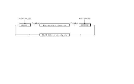
Figure 1: The schematic diagram of creating entangled coherent states for two distant BECs via EIT. Two pairs of coupling and probe lasers are applied on two BECs, respectively. The entangled source produces two entangled probe lasers. After leaving two BECs, the two outgoing probe lasers enter Bell state analyzer to perform projective measurements.

The free evolution of the two quantized probe laser fields is governed by the Hamiltonian

$$\hat{H}_{Pn}=\sum^{2}_{n=1}\left(\hbar\omega_{n}\hat{a}^{\dagger}_{n}\hat{a}_{n}\right),$$ (2)

where $\omega_{n}$ is the frequency of the $n$-th probe laser, and $\hat{a}^{\dagger}_{n}$ and $\hat{a}_{n}$ are the corresponding photon creation and annihilation operators for the $n$-th probe laser field, satisfying the boson communication relation $[\hat{a}_{n},\hat{a}^{\dagger}_{n}]=1$.

The free atomic Hamiltonian is given by

$$\hat{H}_{An} = \sum^{3}_{i=0}\int d{\bf x}\hat{\psi}^{\dagger}_{in}({\bf x})\hat{H}_{in}\hat{\psi}_{in}({\bf x}),$$

$$\hat{H}_{in} = -\frac{\hbar^{2}}{2m}\nabla^{2}+V_{in}({\bf x})+E_{in},$$ (3)

where $E_{in}$ are internal energies for the three internal states, $\hat{\psi}_{in}({\bf x})$ and $\hat{\psi}^{\dagger}_{in}({\bf x})$ are the boson annihilation and creation operators for the $|i\rangle$-state atoms at position ${\bf x}$ for the $n$-th BEC, respectively, they satisfy the standard boson commutation relation $[\hat{\psi}_{in}({\bf x}),\hat{\psi}^{\dagger}_{jm}({\bf x}^{\prime})]=\delta_{ij}\delta_{nm}\delta({\bf x}-{\bf x}^{\prime})$ and $[\hat{\psi}_{in}({\bf x}),\hat{\psi}_{jm}({\bf x}^{\prime})]=0$, and $[\hat{\psi}^{\dagger}_{in}({\bf x}),\hat{\psi}^{\dagger}_{jm}({\bf x}^{\prime})]=0$.

The atom-laser interactions in the dipole approximation can be described by the following Hamiltonian

$$\hat{H}_{In} = -\hbar\int d{\bf x}\left[g_{n}\hat{a}_{n}\hat{\psi}^{\dagger}_{2n}({\bf x})\hat{\psi}_{1n}({\bf x})e^{i({\bf k_{1}}\cdot{\bf x}-\omega_{1}t)}\right.$$ (4)

$$\left.+\frac{1}{2}\Omega_{n}\hat{\psi}^{\dagger}_{2n}({\bf x})\hat{\psi}_{3n}({\bf x})e^{i({\bf k_{2}}\cdot{\bf x}-\omega_{2}t)}+\tt{H.c.}\right],$$

where dipole coupling constants are defined by $g_{n}=\mu_{21}{\cal E}_{1n}/\hbar$ and $\Omega_{n}=\mu_{23}E_{2n}/\hbar$ with $\mu_{ij}$ denoting a transition dipole-matrix element between states $|i\rangle$ and $|j\rangle$, ${\cal E}_{1n}=\sqrt{\hbar\omega_{1n}/2\epsilon_{0}V}$ being the electric field per photon for the quantized probe light of frequency $\omega_{1n}$ in a mode volume $V$, and $E_{2n}$ being the amplitude of the electric field for the classical coupling light of frequency $\omega_{2}$, ${\bf k}_{1n}$ and ${\bf k}_{2n}$ are wave vectors of correspondent laser fields.

The interatomic collision Hamiltonian is taken to be the following form

$$\hat{H}_{Cn} = \frac{2\pi\hbar^{2}}{m}\int d{\bf x}\left[\sum^{3}_{i=1}a^{sc}_{in}\hat{\psi}^{\dagger}_{in}({\bf x})\hat{\psi}^{\dagger}_{in}({\bf x})\hat{\psi}_{in}({\bf x})\hat{\psi}_{in}({\bf x})\right.$$ (5)

$$\left.+\sum_{i\neq j}2a^{sc}_{ij}\hat{\psi}^{\dagger}_{in}({\bf x})\hat{\psi}^{\dagger}_{jn}({\bf x})\hat{\psi}_{in}({\bf x})\hat{\psi}_{jn}({\bf x})\right],$$

where $a^{sc}_{i}$ is the $s$-wave scattering length of condensed atoms in the internal state $|i\rangle$ and $a^{sc}_{ij}$ that between condensed atoms in the internal states $|i\rangle$ and $|j\rangle$.

Figure 2: Three-level $\Lambda$-type atoms coupled to two laser fields with the detunings $\Delta_{1}$ and $\Delta_{2}$, respectively.

For a weakly interacting BEC at zero temperature there are no thermally excited atoms and the quantum depletion is negligible, the motional state is frozen to be approximately the ground state. One may neglect all modes except for the condensate mode and approximately factorize the atomic field operators as $\hat{\psi}_{in}({\bf x})\approx\hat{b}_{in}\phi_{in}({\bf x})$ where $\phi_{in}({\bf x})$ is a normalized wavefunction for the atoms in the BEC in the internal state $|i\rangle$, which is given by the ground state of the following Schrödinger equation

$$\left[-\frac{\hbar^{2}}{2m}\nabla^{2}+V_{in}({\bf x})+E_{in}\right]{\phi}_{in}({\bf x})=\hbar\nu_{in}{\phi}_{in}({\bf x}),$$ (6)

where $\hbar\nu_{in}$ is the energy of the mode $i$, and $\nu_{in}$ denotes the frequency to the free evolution of the condensate in the internal state $|i\rangle$.

Substituting the single-mode expansions of the atomic field operators into Eqs. (II-5), we arrive at the following approximate Hamiltonian

$$\hat{H}=\hat{H}_{1}+\hat{H}_{2},$$ (7)

where the two commutable parts of the Hamiltonian are given by

$$\hat{H}_{n} = \hbar\omega_{n}\hat{a}^{\dagger}_{n}\hat{a}_{n}+\hbar\sum^{3}_{i=1}\nu_{in}\hat{b}^{\dagger}_{in}\hat{b}_{in}$$ (8)

$$-\hbar\left[g_{1n}\hat{a}_{n}\hat{b}^{\dagger}_{2n}\hat{b}_{1n}e^{-i\omega_{1}t}+g_{2n}\hat{b}^{\dagger}_{2n}\hat{b}_{3n}e^{-i\omega_{2}t}+\tt{H.c.}\right]$$

$$+\hbar\sum^{3}_{i=1}\lambda_{in}\hat{b}^{\dagger 2}_{in}\hat{b}^{2}_{in}+\hbar\sum_{i\neq j}\lambda_{ijn}\hat{b}^{\dagger}_{in}\hat{b}_{in}\hat{b}^{\dagger}_{jn}\hat{b}_{jn},$$

where the modes $\hat{a}_{n}$ ($n=1,2$) correspond to the two probe laser fields, the modes $\hat{b}_{in}$ ($n=1,2,$ and $i=1,2,3$) to atomic fields in the three internal state, respectively. Here $g_{1n}$ and $g_{2n}$ denote the laser-atom dipole interactions. They are defined by

$$g_{1n} = g_{n}\int d{\bf x}\phi^{*}_{2n}({\bf x})\phi_{1n}({\bf x})e^{i{\bf k}_{1}.{\bf x}},$$

$$g_{2n} = \frac{1}{2}\Omega_{n}\int d{\bf x}\phi^{*}_{2n}({\bf x})\phi_{3n}({\bf x})e^{i{\bf k}_{2}.{\bf x}}.$$ (9)

And $\lambda_{in}$ and $\lambda_{ijn}$ ($i,j=1,2,3$) describe interatomic interactions ($s$-wave elastic scattering) given by

$$\lambda_{ijn} = \frac{4\pi\hbar^{2}a^{sc}_{ij}}{m}\int d{\bf x}|\phi_{in}({\bf x})|^{2}|\phi_{jn}({\bf x})|^{2},\hskip 8.5359pt(i\neq j),$$

$$\lambda_{in} = \frac{2\pi\hbar^{2}a^{sc}_{i}}{m}\int d{\bf x}|\phi_{in}({\bf x})|^{4}.$$ (10)

Properly choosing a unitary transformation, we can transfer the time-dependent Hamiltonian (7) to the following time-independent Hamiltonian

$$\hat{H}_{I}=\hat{H}_{I1}+\hat{H}_{I2},$$ (11)

where $\hat{H}_{In}$ ($n=1,2$) can take the following form

$$\hat{H}_{In} = \hbar(\Delta_{1n}-\Delta_{2n})\hat{b}^{\dagger}_{3n}\hat{b}_{3n}+\Delta_{1n}\hat{b}^{\dagger}_{2n}\hat{b}_{2n}$$ (12)

$$-\hbar[g_{1n}\hat{a}_{1}\hat{b}^{\dagger}_{2n}\hat{b}_{1n}+g_{2n}\hat{b}^{\dagger}_{2n}\hat{b}_{3n}+\tt{H.c.}]$$

$$+\hbar\sum^{3}_{i=1}\lambda_{in}\hat{b}^{\dagger 2}_{in}\hat{b}^{2}_{in}+\hbar\sum_{i\neq j}\lambda_{ijn}\hat{b}^{\dagger}_{in}\hat{b}_{in}\hat{b}^{\dagger}_{jn}\hat{b}_{jn},$$

where $\Delta_{1n}=\nu_{2n}-\nu_{1n}-\omega_{1n}$ and $\Delta_{2n}=\nu_{2n}-\nu_{3n}-\omega_{2n}$ are the detunings of the corresponding probe and coupling laser beams, respectively.

We consider the situation of the ideal EIT which is attained only when the system is at the two-photon resonance with the detuning $\Delta=\Delta_{1n}=\Delta_{2n}$ and the involved lasers are applied adiabatically. Initially the lasers are outside the BEC medium in which all atoms are in their ground state, i.e., the internal state $|1\rangle_{i}$ ($i=1,2$). These condensed atoms are generally in a superposition state of the state $|1\rangle_{i}$ and the state $|3\rangle_{i}$ when they are in EIT. However, when the coupling laser is much stronger than the probe laser, atomic population at the intermediate level approaches zero while the upper level is unpopulated when EIT occurs scul . Hence, when the BECs are in EIT states, under the condition of $(g_{1n}/g_{2n})^{2}<<1$ the terms which involve $\hat{b}^{\dagger}_{2n}\hat{b}_{2n}$ and $\hat{b}^{\dagger}_{3n}\hat{b}_{3n}$ in the Hamiltonian (8) may be neglected, and from the Hamiltonian (8) we can adiabatically eliminate the atomic field operators in the internal states $|2\rangle$ and $|3\rangle$ kua . Then, the resulting effective Hamiltonian contains only the atomic field operators in internal states $|1\rangle_{n}$ and the probe field operators and have the following simple form

$$\hat{H}_{eff}=\sum^{2}_{n=1}\left(\omega^{\prime}_{n}\hat{b}^{\dagger}_{n}\hat{b}_{n}+2\omega^{\prime}_{n}\hat{b}^{\dagger}_{n}\hat{b}_{n}\hat{a}^{\dagger}_{n}\hat{a}_{n}+\lambda_{n}\hat{b}^{\dagger 2}_{n}\hat{b}^{2}_{n}\right),$$ (13)

where we have set $\hat{b}_{n}=\hat{b}_{1n}$, $\hat{b}^{\dagger}_{n}=\hat{b}^{\dagger}_{1n}$ and $\lambda_{n}=\lambda_{1n}$ for the simplification of notations, and we have also taken $\hbar=1$ and introduced

$$\omega^{\prime}_{n}=-\frac{2|g_{1n}|^{2}}{\Delta_{1n}}.$$ (14)

Obviously, the effective four-mode Hamiltonian (13) is diagonal in the Fock space with the bases defined by

$$|n_{1},n_{2},m_{1},m_{2}\rangle=\frac{\hat{a}^{\dagger n_{1}}_{1}\hat{a}^{\dagger n_{2}}_{2}\hat{b}^{\dagger m_{1}}_{1}\hat{b}^{\dagger m_{2}}_{2}}{\sqrt{n_{1}!n_{2}!m_{1}!m_{2}!}}|0,0,0,0\rangle,$$ (15)

which are eigenstates of the effective Hamiltonian with the eigenvalues given by the following expression

$$E_{n_{1},n_{2},m_{1},m_{2}}=\sum^{2}_{i=1}\left[\omega^{\prime}_{i}m_{i}+2\omega^{\prime}_{i}n_{i}m_{i}+\lambda_{i}m_{i}(m_{i}-1)\right],$$ (16)

where $n_{i}$ and $m_{i}$ take non-negative integers.

It should be mentioned that in most textbooks on EIT scul ; ari , both the probe and coupling lasers are treated classically, the decay of excited states is included in the dynamics of the internal states through a set of density-matrix equations of the atomic system, the decay promotes the trapping of the atom into a dark state. Contrary to the usual treatment of EIT, the probe laser is quantized in present paper. A limitation of our present treatment is that we have ignored the decay rates of various levels. However, this ignorance of the decay rates is a good approximation for the adiabatic EIT that we study in the present paper, since the adiabatic EIT is insensitive to any possible decay of the top level lm .

III Generation of entangled state between photons and distant BECs

In this section, as one of the key ingredients to create entangled coherent states of the two distant BECs we investigate the generation of atom-photon entangled state between the two probe laser fields and two distant BEC system in terms of analytic solution obtained in the previous section. Since there does not exist direct interaction between the two distant BECs under our consideration, entangled states between them can not be created through interaction between two distant BECs if they are initially not entangled. However, if the two probe laser fields are initially in an entangled state, it is possible to create entangled state of the two distant BECs through performing appropriate quantum measurements upon output state of the two probe laser fields. In some sense we can say that entanglement is transferred from the two probe laser fields to the two distant BECs. An initial entangled state of the two probe laser fields can be regarded as a quantum channel to create quantum entanglement between the two distant BECs. Once the quantum channel is given, one of important steps of creating entangled distant BECs is to generate photon-atom entangled state. In order to be specific, we here use an entangled single-photon channel to show how to create a hybrid entangled state between the two probe laser fields and two distant BECs to make preparation for obtaining entangled states of distant BECs which will be discussed in the next section.

We assume that the two distant BECs are initially uncorrelated and they are in a two-mode product coherent state $|\alpha_{1},\alpha_{2}\rangle\equiv|\alpha_{1}\rangle\otimes|\alpha_{2}\rangle=D_{\hat{b}_{1}}(\alpha_{1})D_{\hat{b}_{2}}(\alpha_{2})|0,0\rangle$ with the displacement operators being defined by $D_{\hat{b}_{i}}(\alpha_{i})=\exp(\alpha_{i}\hat{b}^{\dagger}_{i}-\alpha^{*}_{i}\hat{b}_{i})$, while the entangling source produces a pair of the probe lasers which is in the entangled single-photon state

$$|{\tt B}(\theta,\varphi)\rangle=\cos\theta|0,0\rangle+\sin\theta e^{i\varphi}|1,1\rangle.$$ (17)

Then the joint initial state of the atom-photon system is given by

$$|\Phi(0)\rangle=|{\tt B}(\theta,\varphi)\rangle\otimes|\alpha_{1},\alpha_{2}\rangle.$$ (18)

Assume that the lasers are adiabatically applied at the time of $t=0$, then from Eqs. (13-18) it is straightforward to show that after an interaction time $t$ the joint state of the system will be given by

$$|\Phi(t)\rangle = \cos\theta|0,0\rangle\otimes|\phi_{\alpha_{1}\alpha_{2}}(t)\rangle$$ (19)

$$+\sin\theta e^{i\varphi}|1,1\rangle\otimes|\phi^{\prime}_{\alpha_{1}\alpha_{2}}(t)\rangle,$$

where we have introduced two wave functions for the two distant BECs

$$|\phi_{\alpha_{1}\alpha_{2}}(t)\rangle = |\phi_{\alpha_{1}}(t)\rangle\otimes|\phi_{\alpha_{2}}(t)\rangle,$$

$$|\phi^{\prime}_{\alpha_{1}\alpha_{2}}(t)\rangle = |\phi^{\prime}_{\alpha_{1}}(t)\rangle\otimes|\phi^{\prime}_{\alpha_{2}}(t)\rangle,$$ (20)

where the two wave functions of the single BECs are defined by

$$|\phi_{\alpha_{i}}(t)\rangle = \exp\left\{-it[\omega^{\prime}_{i}\hat{n}_{b_{i}}+\lambda_{i}\hat{n}_{b_{i}}(\hat{n}_{b_{i}}-1)]\right\}|\alpha_{i}\rangle,$$

$$|\phi^{\prime}_{\alpha_{i}}(t)\rangle = \exp\left\{-it[3\omega^{\prime}_{i}\hat{n}_{b_{i}}+\lambda_{i}\hat{n}_{b_{i}}(\hat{n}_{b_{i}}-1)]\right\}|\alpha_{i}\rangle.$$ (21)

In the following we shall see that starting with the state given by Eq. (19), different atom-photon entangled states can be obtained at different evolution times of the joint system under our consideration through adjusting various interaction strengths and the detunings. In order to see this, for simplicity we suppose that $g_{1n}=g_{2n}=g$, $\omega^{\prime}_{1}=\omega^{\prime}_{2}=\omega^{\prime}$, $\lambda_{1}=\lambda_{2}=\lambda$, and introduce a scaled time $\tau=\lambda t$, then the states of the single BECs given by Eq. (III) become the following generalized coherent states tit ; bia ; sto

$$|\phi_{\alpha_{i}}(\tau)\rangle = e^{-|\alpha_{i}|^{2}/2}\sum^{\infty}_{m_{i}=0}e^{i\tau\theta_{m_{i}}}\frac{\alpha^{m_{i}}_{i}}{\sqrt{m_{i}!}}|m_{i}\rangle,$$

$$|\phi^{\prime}_{\alpha_{i}}(\tau)\rangle = e^{-|\alpha_{i}|^{2}/2}\sum^{\infty}_{m_{i}=0}e^{i\tau\theta^{\prime}_{m_{i}}}\frac{\alpha^{m_{i}}_{i}}{\sqrt{m_{i}!}}|m_{i}\rangle,$$ (22)

where two running frequencies $\theta_{m_{i}}$ and $\theta^{\prime}_{m_{i}}$ are defined by

$$\theta_{m_{i}}=(K+1)m_{i}-m^{2}_{i},\hskip 8.5359pt\theta^{\prime}_{m_{i}}=(3K+1)m_{i}-m^{2}_{i},$$ (23)

where we have introduced a real effective interaction parameter $K$ defined by

$$K=-\frac{2|g|^{2}}{\lambda\Delta},$$ (24)

which describes an effective interaction induced by three adjustable parameters of the involved lasers and two distant BECs: the dipole interaction strength $g$, the interatomic interaction strength $\lambda$, and the two-photon detuning $\Delta$. The effective interaction parameter $K$ can takes positive or negative values which depends on the signs of $\lambda$ and $\Delta$. For an atomic BEC with a positive $s$-wave scattering length, $K$ is positive (negative) when the two-photon detuning $\Delta$ is positive (negative). These indicate that there is a large space to adjust values of the effective interaction parameter $K$. From Eqs. (19) to (23) we can see that the time evolution characteristic of the system under our consideration is completely determined by the effective interaction parameter.

These generalized coherent states given by Eq. (III) differ from a conventional Glauber coherent state by an extra phase factor appearing in the decomposition of such states into a superposition of Fock states. They can always be represented as a continuous sum (integral) form of Glauber coherent states. And under appropriate periodic conditions, they can reduce to discrete superpositions of coherent states. In order to see this, we express states given by Eq. (III) as the following integral form

$$|\phi_{\alpha_{i}}(\tau)\rangle = \frac{1}{2\pi}\int^{2\pi}_{0}d\phi_{i}f(\phi_{i},\theta_{m_{i}})\left|\alpha_{i}e^{i\phi_{i}}\right\rangle,$$

$$|\phi^{\prime}_{\alpha_{i}}(\tau)\rangle = \frac{1}{2\pi}\int^{2\pi}_{0}d\phi_{i}f(\phi_{i},\theta^{\prime}_{m_{i}})\left|\alpha_{i}e^{i\phi_{i}}\right\rangle,$$ (25)

where the two phase functions are introduced with the following expressions

$$f(\phi_{i},\theta_{m_{i}}) = \exp\left[i\left(\tau\theta_{m_{i}}-m_{i}\phi_{i}\right)\right],$$

$$f(\phi_{i},\theta^{\prime}_{m_{i}}) = \exp\left[i\left(\tau\theta^{\prime}_{m_{i}}-m_{i}\phi_{i}\right)\right].$$ (26)

It should be kept in mind that we want to create entangled coherent states for two distant BECs what we expect. Eq. (III) indicates that both the state $|\phi_{\alpha_{1}\alpha_{2}}(\tau)\rangle$ and the state $|\phi^{\prime}_{\alpha_{1}\alpha_{2}}(\tau)\rangle$ are continuous superposition states of two-mode product coherent states. From Eqs. (III-III) we can see that the values of the effective interaction parameter $K$ may seriously affect the form of the states given by Eq. (III). Of particular interesting is the situation where $K$ takes values of nonzero integers. In this case, both $\theta_{m_{i}}$ and $\theta^{\prime}_{m_{i}}$ take integers. Making use of Eq. (III) and Eq. (23), from Eqs. (19) and (III) we can see that $|\Phi(\tau+2\pi)\rangle=|\Phi(\tau)\rangle$, which implies that the time evolution of the joint wavefunction given by Eq. (19) is a periodic evolution with respect to the scaled time $\tau$ with the period $2\pi$. On the other hand, suppose that the scaled interaction time $\tau$ takes its values in the following manner

$$\tau=\frac{M}{N}2\pi,$$ (27)

where $M$ and $N$ are mutually prime integers, then we can find that

$$f(\phi_{i},\theta_{m_{i}}) = f(\phi_{i},\theta_{m_{i}+N}),$$

$$f(\phi_{i},\theta^{\prime}_{m_{i}}) = f(\phi_{i},\theta^{\prime}_{m_{i}+N}),$$ (28)

which means that the two exponential phase functions in the states given by Eq. (III) are also periodic functions with respect to $m_{i}$ with the same period $N$. If $\tau$ takes its values according to Eq. (27), as a fraction of the period, then the two states given by Eq. (III) become discrete superposition states of product coherent states, and they can be expressed as follows

$$\left|\phi_{\alpha_{1}\alpha_{2}}\left(\tau=2\pi M/N\right)\right\rangle = \prod^{2}_{i=1}\sum^{N}_{r_{i}=1}c_{r_{i}}\left|\alpha_{i}e^{i\varphi_{r_{i}}}\right\rangle,$$

$$\left|\phi^{\prime}_{\alpha_{1}\alpha_{2}}\left(\tau=2\pi M/N\right)\right\rangle = \prod^{2}_{i=1}\sum^{N}_{r_{i}=1}c^{\prime}_{r_{i}}\left|\alpha_{i}e^{i\varphi_{r_{i}}}\right\rangle,$$ (29)

the running phase is defined by the following expression

$$\varphi_{r_{i}}=\frac{2\pi}{N}r_{i},\hskip 14.22636pt(r_{i},=1,2,\cdots,N),$$ (30)

and different superposition coefficients are given by

$$c_{r_{i}} = \frac{1}{N}\sum^{N}_{m_{i}=1}\exp\left\{-\frac{2\pi i}{N}\left[m_{i}r_{i}-M\theta_{m_{i}}\right]\right\},$$

$$c^{\prime}_{r_{i}} = \frac{1}{N}\sum^{N}_{m_{i}=1}\exp\left\{-\frac{2\pi i}{N}\left[m_{i}r_{i}-M\theta^{\prime}_{m_{i}}\right]\right\}.$$ (31)

Now it is easy to see that after an interaction time $\tau=2\pi M/N$ with the lasers the joint state given by Eq. (19) becomes

$$\left|\Phi\left(\tau=\frac{M}{N}2\pi\right)\right\rangle = \cos\theta|0,0\rangle\otimes\sum^{N}_{r_{1},r_{2}=1}c_{r_{1}}c_{r_{2}}|\alpha_{1}e^{i\varphi_{r_{1}}},\alpha_{2}e^{i\varphi_{r_{2}}}\rangle$$ (32)

$$+\sin\theta e^{i\varphi}|1,1\rangle\otimes\sum^{N}_{r_{1},r_{2}=1}c^{\prime}_{r_{1}}c^{\prime}_{r_{2}}|\alpha_{1}e^{i\varphi_{r_{1}}},\alpha_{2}e^{i\varphi_{r_{2}}}\rangle.$$

The state given by Eq. (32) is generally an atom-photon entangled state between the two probe laser fields and the two distant BECs. It is interesting to note that it is a hybrid entangled state in which one subsystem (photon) is discrete while another (BEC) is continuous, since it exhibits quantum entanglement between two distinct degrees of freedom mon ; bru ; chen ; hal . In principle, hybrid entangled state can serve as a valuable resource in quantum information processing and build up a bridge between quantum information protocols of discrete and continuous variables. As a specific example of creating atom-photon hybrid entangled states, we discuss the case of $K=1$. Assume that the probe lasers and the condensates are initially in the state given by (18) with $\theta=\pi/4$ and $\varphi=0$. When $K=1$, $N=4$, and $M=1$, from Eqs. (III) and (32) we find that after the interaction times $\tau=\pi/2$ the joint wave function given by Eq. (32) becomes the following hybrid entangled state

$$|\Phi(\tau=\pi/2)\rangle = \mathcal{N}\left[|B(\pi/4,0)\rangle\otimes|E(\alpha_{1},-\alpha_{2})\rangle\right.$$ (33)

$$\left.+i|B(-\pi/4,0)\rangle\otimes|E(\alpha_{1},\alpha_{2})\rangle\right],$$

where $|B(\pm\pi/4,0)\rangle$ are two optical Bell states defined by

$$|B(\pm\pi/4,0)\rangle=\frac{1}{\sqrt{2}}(|0,0\rangle\pm|1,1\rangle),$$ (34)

while $|E(\alpha_{1},\pm\alpha_{2})\rangle$ are two normalized entangled coherent states hir for the two BECs, they are defined by

$$|E(\alpha,\beta)\rangle=\frac{1}{\sqrt{N_{\alpha\beta}}}(|\alpha,\beta\rangle+|-\alpha,-\beta\rangle),$$ (35)

where the normalized constant is given by

$$N_{\alpha\beta}=2\left\{1+\exp[-2(|\alpha|^{2}+|\beta|^{2})]\right\},$$ (36)

which gives the normalized constant in Eq. (33) by the form $\mathcal{N}=(N_{\alpha\beta}/2)^{1/2}$. When $\beta=\pm\alpha$, the two states $|E(\alpha_{1},\pm\alpha_{2})\rangle$ become quasi-Bell states which will defined in the next section.

Atom-photon entangled states given by Eqs. (32) and (33) are important results of the present paper. They indicate that we can deterministically generate atom-photon entangled states between the two probe lasers and the two distant BECs. In particular, we note that the entangled state given by Eq. (33) is of three interesting characters. First of all, the state given by Eq. (33) is a hybrid entangled state between atoms and photons where atoms and photons are entangled, photons are well suited for transmission over long distances and carry away information on the state of atoms while atoms have the advantage of being more easily stored. Such an entangled state provides a possibility for a communication link in a quantum network. Secondly, the state given by Eq. (33) is a type of entangled states between two pairs of entangled states where one entangled pair is Bell states of photons while the other is entangled coherent states of atoms. In particular, when $\alpha_{2}=\pm\alpha_{1}$,it is an entangled state between a pair of optical Bell states and a pair of atomic quasi-Bell states. The practical development of such kind of entangled states is of importance for exploring quantum nonlocality and testing Bell’s inequality. Thirdly, the state given by Eq. (33) is also a hybrid entangled state between discrete-variable states and continuous variable states, such a kind of entangled states may open new ways to carry out quantum information processing. In what follows we will observe that these atom-photon entangled states in this section produced give a supply for the generation of entangled coherent states of the two distant BECs which will be investigated in the next section.

IV Generation of entangled coherent states for distant BECs

From the discussions of the previous section we can see that different atom-photon entangled states between the probe lasers and the two distant BECs can be obtained using different initial entangled states (quantum channels) of the probe lasers. In this section we study the generation of entangled coherent states of the two distant BECs using different quantum channels. Concretely, we will propose two schemes to create entangled coherent states of the two distant BECs. One is a single-photon scheme, the other is a multiphoton scheme. An entangled single-photon state is used to serve the quantum channel in the single-photon protocol while an entangled coherent-state acts as the quantum channel in the multiphoton scheme.

A. The entangled single-photon-state scheme

In this subsection we discuss how to produce entangled coherent states between two distant BECs using the single-photon quantum channel. In this case, the two probe lasers are initially in the entangled single-photon state $|B(\theta,\varphi)\rangle$ given by Eq. (17) in which there is an one-photon state in each probe mode while the two BECs are initially in a product coherent state. Then the joint initial state of the atom-photon system is given by (18). We note that at a time $t$ the state of the system under our consideration is given by (19), and it can be expressed in terms of optical Bell bases of probe photons as the following form

$$|\Phi(t)\rangle = \frac{1}{\sqrt{2}}[|B(\pi/4,0)\rangle\otimes|\psi_{\alpha_{1}\alpha_{2}}(t)\rangle_{+}$$ (37)

$$+|B(-\pi/4,0)\rangle\otimes|\psi_{\alpha_{1}\alpha_{2}}(t)\rangle_{-}],$$

where $|B(\pm\pi/4,0)\rangle$ are two optical Bell states defined by Eq. (34) and we introduce the following superposition states of the two BECs

$$|\psi_{\alpha_{1}\alpha_{2}}(t)\rangle_{\pm}=\cos\theta|\phi_{\alpha_{1}\alpha_{2}}(t)\rangle\pm\sin\theta e^{i\varphi}|\phi^{\prime}_{\alpha_{1}\alpha_{2}}(t)\rangle,$$ (38)

where states $|\phi_{\alpha_{1}\alpha_{2}}(t)\rangle$ and $|\phi^{\prime}_{\alpha_{1}\alpha_{2}}(t)\rangle$ are defined in Eq. (III), they are not entangled states during the time evolution of the whole system under our consideration.

Starting with the state given by Eq. (37), we can see that the superposition states of the two distant BECs defined by Eq. (38) can be probabilistically produced through performing optical Bell measurements upon the outgoing states of the two probe lasers. From the discussions of the previous section we can see that both $|\phi_{\alpha_{1}\alpha_{2}}(t)\rangle$ and $|\phi^{\prime}_{\alpha_{1}\alpha_{2}}(t)\rangle$ are generally superposed coherent states. Hence, in general the states $|\psi_{\alpha_{1}\alpha_{2}}(t)\rangle_{+}$ and $|\psi_{\alpha_{1}\alpha_{2}}(t)\rangle_{-}$ are entangled coherent states. In particular, when $\tau=2\pi M/N$ with $M$ and $N$ being prime numbers, we have the following entangled coherent states

$$|\psi_{\alpha_{1}\alpha_{2}}(\tau=2\pi M/N)\rangle_{\pm}=\sum^{N}_{r_{1},r_{2}=1}C^{\pm}_{r_{1}r_{2}}|\alpha_{1}e^{i\varphi_{r_{1}}}\rangle|\alpha_{2}e^{i\varphi_{r_{2}}}\rangle,$$ (39)

where the superposed coefficients are given by

$$C^{\pm}_{r_{1}r_{2}}=\cos\theta c_{r_{1}}c_{r_{2}}\pm\sin\theta e^{i\varphi}c^{\prime}_{r_{1}}c^{\prime}_{r_{2}}.$$ (40)

It is interesting to note that the entangled coherent states given by Eq. (39) are higher-dimensional entangled coherent states which are superposed states of $N^{2}$ linearly independent product coherent states $|\alpha_{1}e^{i\varphi_{r_{1}}}\rangle|\alpha_{2}e^{i\varphi_{r_{2}}}\rangle$ with $r_{i}=1,2,\cdots,N$ and $i=1,2$. However, from Eqs. (38-40) we can also see that when the two probe lasers are initially not entangled, i.e., $\theta=k\pi$ or $\theta=(2k+1)\pi/2$ with $k$ being an arbitrary integer, the states given by Eqs. (38) and (39) are not entangled states. This means that only when the two probe lasers are initially entangled, it is possible to generate entangled states of the two distant BECs through performing optical Bell measurements. In this sense we can say that quantum entanglement between the two probe lasers is transferred to the two distant BECs through performing optical Bell measurements.

In order to be more specific, let us consider the case of $K=1$, $N=4$, and $M=1$. From Eq. (19) and Eq. (III) we find the atom-photon state is given by Eq. (30). Substituting Eq. (III) into Eq. (38) we arrive at the following entangled coherent states between the two distant BECs

$$|\psi_{\alpha_{1}\alpha_{2}}(\tau=\pi/2)\rangle_{\pm} = C_{\pm}(\theta,\varphi)||E(\alpha_{1},-\alpha_{2})\rangle$$ (41)

$$+iC_{\mp}(\theta,\varphi)||E(\alpha_{1},\alpha_{2})\rangle,$$

where $C_{\pm}(\theta,\varphi)=\cos\theta\pm\sin\theta e^{i\varphi}$, and $||E(\alpha_{1},\pm\alpha_{2})\rangle\equiv|\alpha_{1},\pm\alpha_{2}\rangle+|\pm\alpha_{1},\alpha_{2}\rangle$ are two un-normalized entangled coherent states.

Especially, the state given by Eq. (41) indicates that for the case of $K=1$ if initially the two probe lasers is in an optical Bell state given by Eq. (17) with $\theta=\pi/4$ and $\varphi=0$, then after an interaction time $\tau=\pi/2$ optical Bell measurements upon the two outgoing probe lasers can induce the following two-state entangled coherent states between the two distant BECs (after normalization)

$$\left|\psi_{\alpha_{1}\alpha_{2}}(\tau=\pi/2)\right\rangle_{\pm} = |E(\alpha_{1},\mp\alpha_{2})\rangle,$$ (42)

where $|E(\alpha_{1},\pm\alpha_{2})\rangle$ are entangled coherent states defined in Eq. (35). They are quantum superpositions of four macroscopically distinguishable and linearly independent coherent states $|\alpha_{1},\alpha_{2}\rangle$, $|\alpha_{1},-\alpha_{2}\rangle$, $|\alpha_{1},-\alpha_{2}\rangle$, and $|-\alpha_{1},-\alpha_{2}\rangle$. This means that quantum entanglement of the two single photons in the two probe-laser modes can induce the probabilistic generation of atomic entangled coherent states for the two distant BECs through projective measurements.

Figure 3: The schematic diagram of creating an entangled single-photon state given by Eq. (17) from two-pairs of two-mode squeezed vacuum states by using two beam splitters and two on-off photon detectors.

The preparation of the entangled single-photon state given by Eq. (17) and Bell measurements of optical Bell states $|B(\pm\pi/4,0)\rangle$ given by Eq. (34) are significant ingredients in the present single-photon scheme. As for the preparation of these optical Bell states, Browne et al. bro ; daf have developed a simple protocol to generate the entangled single-photon state given by Eq. (17) using only beam splitters and on-off photon detectors from two pairs of two-mode squeezed vacuum states. The setup of the BEST protocol bro is indicated in Fig. 3 which consists of two beam splitters, two on-off photon detectors. Modes 1 and 2, modes 3 and 4 are fed with weak two-mode squeezed vacuum states $(1-q^{2})\Sigma_{n,m}q^{n+m}|n,n\rangle_{12}\otimes|m,m\rangle_{34}$, which can be approximately expressed as the following un-normalized state (up to the order of $q^{2}$)

$$|\psi_{q}\rangle_{1234} \approx |0000\rangle+q(|0011\rangle+|1100\rangle)$$ (43)

$$+q^{2}(|0022\rangle)+|1111\rangle+|2200\rangle),$$

where the parameter $q=\tanh(r)$ ($0\leq q\ll 1$) is determined by the squeezing parameter $r$. Such states with low values of $r$ are easily produced in experiments. For instance, two-mode squeezed vacuum states have been used to demonstrate experimentally quantum teleportation of a coherent state fur and quantum dense coding with continuous variables miz . In these experiments the squeezing parameter takes its values of $r\simeq 0.35$ and $0.23$, respectively.

Let $\hat{U}_{1}(r_{1},t_{1})$ and $\hat{U}_{2}(r_{2},t_{2})$ denote unitary transformations of the two beam splitters with transmissivity $t_{1}$ and $t_{2}$, and reflectivity $r_{1}$ and $r_{2}$, which satisfy the relation $|r_{i}|^{2}+|t_{i}|^{2}=1$ with $i=1,2$. The two beam-splitter transformations are given by

$$\hat{U}_{1}(r_{1},t_{1}) = t_{1}^{a^{{\dagger}}_{1}a_{1}}e^{-r^{*}_{1}a^{{\dagger}}_{3}a_{1}}e^{r_{1}a_{3}a^{{\dagger}}_{1}}t_{1}^{-a^{{\dagger}}_{3}a_{3}},$$

$$\hat{U}_{2}(r_{1},t_{2}) = t_{1}^{a^{{\dagger}}_{2}a_{2}}e^{-r^{*}_{2}a^{{\dagger}}_{4}a_{2}}e^{r_{2}a_{4}a^{{\dagger}}_{2}}t_{2}^{-a^{{\dagger}}_{4}a_{4}},$$ (44)

which produce the output state of the two beam splitters given by $\hat{U}_{1}(r_{1},t_{1})\hat{U}_{2}(r_{2},t_{2})|\psi_{q}\rangle_{1234}$ with the following expression

$$|00\rangle_{13}\times|00\rangle_{24}$$

$$+q(r_{1}|10\rangle+t^{*}_{1}|01\rangle)_{13}\times(r_{2}|10\rangle+t^{*}_{2}|01\rangle)_{24}$$

$$+q(t_{1}|10\rangle-r^{*}_{1}|01\rangle)_{13}\times(t_{2}|10\rangle-r^{*}_{2}|01\rangle)_{24}$$

$$+\frac{1}{2}q^{2}\left(\sqrt{2}r^{2}_{1}|20\rangle+\sqrt{2}t^{*2}_{1}|02\rangle+2r_{1}t^{*}_{1}|11\rangle\right)_{13}$$

$$\otimes\left(\sqrt{2}r^{2}_{2}|20\rangle+\sqrt{2}t^{*2}_{2}|02\rangle+2r_{2}t^{*}_{2}|11\rangle\right)_{24}$$

$$+q^{2}\left[\sqrt{2}t_{1}r_{1}|20\rangle-\sqrt{2}t^{*}_{1}r{*}_{1}|02\rangle+(1-2|r_{1}|^{2})|11\rangle\right]_{13}$$

$$\otimes\left[\sqrt{2}t_{2}r_{2}|20\rangle-\sqrt{2}t^{*}_{2}r{*}_{2}|02\rangle+(1-2|r_{2}|^{2})|11\rangle\right]_{24}$$

$$+\frac{1}{2}q^{2}\left[\sqrt{2}t^{2}_{1}|20\rangle-\sqrt{2}r^{*2}_{1}|02\rangle-2t_{1}r^{*}_{1}|11\rangle\right]_{13}$$

$$\otimes\left[\sqrt{2}t^{2}_{2}|20\rangle-\sqrt{2}r^{*2}_{2}|02\rangle-2t_{2}r^{*}_{2}|11\rangle\right]_{24}.$$ (45)

In the derivation of Eq. (IV) we have used the following transformation relations for photonic creation operators of the incoming fields sche ; leon

$$\hat{U}_{1}\left(\begin{array}[]{c}a^{{\dagger}}_{1}\\ a^{{\dagger}}_{3}\\ \end{array}\right)\hat{U}^{{\dagger}}_{1} = \left(\begin{array}[]{cc}t_{1}&-r^{*}_{1}\\ r_{1}&t^{*}_{1}\\ \end{array}\right)\left(\begin{array}[]{c}a^{{\dagger}}_{1}\\ a^{{\dagger}}_{3}\\ \end{array}\right),$$ (52)

$$\hat{U}_{2}\left(\begin{array}[]{c}a^{{\dagger}}_{2}\\ a^{{\dagger}}_{4}\\ \end{array}\right)\hat{U}^{{\dagger}}_{2} = \left(\begin{array}[]{cc}t_{2}&-r^{*}_{2}\\ r_{2}&t^{*}_{2}\\ \end{array}\right)\left(\begin{array}[]{c}a^{{\dagger}}_{2}\\ a^{{\dagger}}_{4}\\ \end{array}\right).$$ (59)

The on-off detectors distinguish between vacuum and the presence of any number photons. An ideal on-off detection with quantum efficiency $\eta=1$ can be described by the positive operator-valued measure (POVM) of each detector $\hat{\Pi}=|0\rangle\langle 0|$ and $\hat{D}=I-|0\rangle\langle 0|$. We consider two on-off detectors with the same quantum efficiency $\eta$ by the operator oli ; sas

$$\hat{D}_{i}(\eta)=\sum^{\infty}_{n=0}(1-\eta)^{n}|n\rangle_{i}|\langle n|,\hskip 28.45274pt(i=1,2).$$ (60)

Then the entangled single-photon state of the form defined by Eq. (17) can be produced for arbitrary values of the parameters $\theta$ and $\varphi$ in Eq. (17) through the procedure indicated in Fig. 3 with the following output state

$$|\Psi\rangle_{1234}=\hat{D}_{1}(\eta)\hat{D}_{2}(\eta)\hat{U}_{1}(r_{1},t_{1})\hat{U}_{2}(r_{2},t_{2})|\psi_{q}\rangle_{1234},$$ (61)

which describes two identical two-mode squeezed states are mixed pairwise at unbalanced beam splitters followed by the on-off photon detections which are indicated in Fig. 3.

Through length but straightforward calculations, making use of Eqs. (IV) and (60) from Eqs. (43) and (61) we can find that

$$|\Psi\rangle_{1234} = q\chi_{1}|0011\rangle+q^{2}[\chi_{2}|1111\rangle+\chi_{3}|1012\rangle$$ (62)

$$+\chi_{4}|0022\rangle+\chi_{5}|0121\rangle],$$

where the five coefficients are given by

$$\chi_{1} = (r^{*}_{1}r^{*}+t^{*}_{1}t^{*}_{2})\eta^{2},$$

$$\chi_{2} = [2r_{1}r_{2}t^{*}_{1}t^{*}_{2}+2t_{1}t_{2}r^{*}_{1}r^{*}_{2}+(1-2|r_{1}|^{2})(1-2|r_{2}|^{2})]\eta^{2},$$

$$\chi_{3} = \sqrt{2}[r_{1}t^{*}_{1}t^{*2}_{2}-r^{*}_{1}t^{*}_{1}r^{*2}_{2}-r^{*}_{2}t^{*}_{2}(1-2|r_{1}|^{2})]\eta^{2}(2-\eta),$$

$$\chi_{5} = \sqrt{2}\left[r_{2}t^{*}_{2}t^{*2}_{1}-t_{2}r^{*}_{2}r^{*2}_{1}-r^{*}_{1}t^{*}_{1}(1-2|r_{2}|^{2})\right]\eta^{2}(2-\eta),$$

$$\chi_{4} = (r^{*}_{1}r^{*}_{2}-t^{*}_{1}t^{*}_{2})^{2}\eta^{2}(2-\eta).$$ (63)

After taking trace of the state (62) over modes 3 and 4, we find the reduced density operator of the normalized state of modes 1 and 2 to be the following form

$$\rho_{12} = P_{\psi}|\psi\rangle_{12}\langle\psi|+P_{10}(|10\rangle_{12}\langle 10|$$ (64)

$$+P_{00}(|00\rangle_{12}\langle 00|+P_{01}(|01\rangle_{12}\langle 01|,$$

where the producing probabilities of the corresponding states are given by

$$P_{\psi} = \frac{|\chi_{1}|^{2}+q^{2}|\chi_{2}|^{2}}{\Sigma},\hskip 8.5359ptP_{10}=\frac{q^{2}|\chi_{3}|^{2}}{\Sigma},$$

$$P_{00} = \frac{q^{2}|\chi_{4}|^{2}}{\Sigma},\hskip 8.5359ptP_{01}=\frac{q^{2}|\chi_{5}|^{2}}{\Sigma},$$ (65)

where we have introduced the symbol

$$\Sigma=|\chi_{1}|^{2}+q^{2}(|\chi_{2}|^{2}+|\chi_{3}|^{2}+|\chi_{4}|^{2}+|\chi_{5}|^{2}),$$ (66)

and the expected state $|\psi\rangle_{12}$ has the following form

$$|\psi\rangle_{12}=\frac{\chi_{1}|00\rangle_{12}+q\chi_{2}|11\rangle_{12}}{\sqrt{|\chi_{1}|^{2}+q^{2}|\chi_{2}|^{2}}},$$ (67)

which is the entangled single-photon state of the form defined by Eq. (17). From the expressions of $\chi_{1}$ and $\chi_{2}$ given by Eq. (IV) we can see that the entangled single-photon state by Eq. (67) is independent of the quantum efficiency of the on-off detectors. This means that the quantum efficiency of the on-off detectors does not affect the fidelity of the prepared state.

From Eqs. (64-67) we can see that the entangled single-photon state (17) or (67) can be near-deterministically produced if $P_{\psi}\approx 1$, $P_{10}\approx 0$, $P_{00}\approx 0$, and $P_{01}\approx 0$. In what follows we show that two optical Bell states defined by Eq. (34) can be obtained using above procedure through properly choosing parameters of the two beam splitters. In order to see this, we choose $t_{2}\approx 0$ and $r_{2}\approx 1$ for the second beam splitter, and take $q\chi_{2}=\pm\chi_{1}$ which leads to $r_{1}\approx\pm q$ and $t_{1}\approx\sqrt{1-q^{2}}$ for the first beam splitter in which $q$ is defined in Eq. (43). In this case, the five coefficients given by Eq. (IV) become

$$\chi_{1} = \pm q\eta^{2},\chi_{2}=\pm q^{-1}\chi_{1},\chi_{4}=q^{2}\eta^{2}(2-\eta),$$

$$\chi_{3} = -\chi_{5}=\mp q\sqrt{2(1-q^{2}}\eta^{2}(2-\eta),$$ (68)

and the entangled single-photon state $|\psi\rangle_{12}$ becomes

$$|\psi\rangle_{12}=\frac{1}{\sqrt{2}}(|00\rangle_{12}\pm|11\rangle_{12}).$$ (69)

which are two optical Bell states defined in Eq. (34). And the success probabilities of the corresponding states in Eq. (IV) become

$$P_{\psi} = \frac{2}{2+q^{2}(4-3q^{2})(2-\eta)^{2}},$$

$$P_{01} = P_{10}=\frac{2q^{2}(1-q^{2})(2-\eta)^{2}}{2+q^{2}(4-3q^{2})(2-\eta)^{2}},$$

$$P_{00} = \frac{q^{4}(2-\eta)^{2}}{2+q^{2}(4-3q^{2})(2-\eta)^{2}},$$ (70)

which indicate that in the weak squeezing regime of $0<q\ll 1$ we can always find $P_{\psi}\approx 1$, $P_{10}\approx 0$, $P_{\psi}\approx 0$, and $P_{01}\approx 0$ due to $0<\eta\leq 1$. In fact, from the expressions of the probabilities given by Eqs. (IV) we can see that the quantum efficiency of the two detectors does not seriously affect the success probability of generating optical Bell states defined in Eq. (17). For instance, when $q=0.1$ and $\eta=1$, we have $P_{\psi}\approx 98.98\%$ while when $q=0.1$ and $\eta=0.7$, we have $P_{\psi}\approx 98.97\%$. Therefore, in the scheme under our consideration optical Bell states (34) can be produced perfectly with the success probability of approaching unity by using two pairs of two-mode squeezed vacuum states in the weak squeezing regime and on-off detections of photons.

It is a nontrivial thing to distinguish two optical Bell states defined by Eq. (34), which are energy-entangled Bell states since they are defined in the energy representation. To our knowledge, there are a few methods for Bell measurements of the polarization-entangled Bell states and the momentum-entangled Bell states of photons sch ; wal , but no scheme is available for Bell measurements of the energy-entangled Bell states of photons. Recent achievements on cavity QED rai provide us with the possibility of distinguishing energy-entangled Bell states of photons. In what follows we show that two optical Bell states defined by Eq. (34) can be distinguished using entanglement in additional auxiliary atomic systems through mapping two optical Bell states into two atomic Bell states. In order to do this, consider two single-mode cavities which are initially fed with one of the two energy-entangled Bell states given by Eq. (34). Each cavity contains a two-level atom. Two atoms in two cavities interact resonantly with two cavity fields with the Hamiltonian

$$H^{\prime}=\hbar\sum^{2}_{r=1}\left[\frac{\omega_{i}}{2}\sigma^{r}_{z}+\omega_{r}a^{{\dagger}}_{r}a_{r}-i\frac{\Omega}{2}(a_{r}\sigma^{r}_{+}-\sigma^{r}_{-}a^{{\dagger}}_{r})\right],$$ (71)

which implies that if the two cavity fields are initially in two optical Bell states given by Eq. (34) and two atoms are initially in the ground state $|g,g\rangle$, then at the time of $\Omega t=\pi$, the state of the field-atom system governed by Eq. (71) becomes

$$|\Psi(\pi)\rangle = \frac{1}{\sqrt{2}}U(\Omega t=\pi)(|0,0\rangle\pm|1,1\rangle)|g,g\rangle$$ (72)

$$= \frac{1}{\sqrt{2}}|0,0\rangle(|g,g\rangle\pm|e,e\rangle),$$

where $U$ is the time evolution operator corresponding to the Hamiltonian (71).

From Eq. (72) we can see that the discrimination of the two optical Bell states given by Eq. (34) is now changed into distinguishing two atomic Bell states $(|g,g\rangle\pm|e,e\rangle)/\sqrt{2}$. Assume that the two atoms in the two cavities are initially in the two atomic Bell stats $(|g,g\rangle\pm|e,e\rangle)/\sqrt{2}$, applying two classical laser fields to the two atoms, it is easy to find that the two atomic Bell states with the $\pi/2$ evolution of the system performs the following transformations

$$\frac{1}{\sqrt{2}}(|g,g\rangle+|e,e\rangle) \rightarrow \frac{1}{\sqrt{2}}(|e,e\rangle+|g,g\rangle)$$

$$\frac{1}{\sqrt{2}}(|g,g\rangle-|e,e\rangle) \rightarrow \frac{1}{\sqrt{2}}(|e,g\rangle-|g,e\rangle),$$ (73)

which indicate that when both of the two atoms in the two cavities are detected to be in the excited state $|e,e\rangle$ or the ground state $|g,g\rangle$, the atomic Bell state $(|g,g\rangle+|e,e\rangle)/\sqrt{2}$ is identified. When one atom is detected to be in the excited state and another to be in the ground state, i.e., $|e,g\rangle$ or $|g,e\rangle$, the atomic Bell state $(|g,g\rangle-|e,e\rangle)/\sqrt{2}$ is identified. This implies the discrimination of the two energy-entangled Bell states of photons given by Eq. (34).

It is worthwhile to mention that the physical mechanism of generating atom-atom entangled states between two distant BECs in this section is very different from that of producing atom-photon entangled states in the previous section. There are two key factors to generate quantum entanglement between two distant BECs. One is that the two probe laser fields must have the initial quantum entanglement as indicated in the above discussion. In this sense the appearance of the entanglement of the two distant BECs is the result of entanglement transferring from the two probe lasers to the two distant BECs through performing optical Bell measurements. The other is that the concrete form of entangled coherent states depends upon the parameters of the applied lasers and the two BECs and the interaction time.

It should be mentioned that one drawback of using the entangled single-photon state as a quantum channel for generating entangled coherent states of distant BECs is that it is extremely sensitive to photon loss and detection inefficiency. In particular, the completely correlated state is destroyed by loss of even a single photon. Other correlated states may have somewhat less strict requirements. In order to overcome this disadvantage in the following we will use the entangled coherent-state channel to create entangled coherent states of distant BECs. Because entangled coherent states are multiphoton states, they are more robust against small levels of photon absorption losses.

B. The entangled coherent-state scheme

In complete analogy to the above discussion, the entangled coherent state channel can be used to create entangled states of distant BECs. In order to see this, we assume that the two distant BECs are initially uncorrelated and they are in a two-mode coherent state $|\alpha_{1},\alpha_{2}\rangle$ while the pair of the probe lasers are initially in the entangled coherent state $|E(\beta,\beta)\rangle_{+}$ defined by Eq. (35) which is a quasi-Bell basis. As well known, for a given nonzero number $\beta$ there are four linearly independent two-mode coherent states $|\beta,\beta\rangle$, $|\beta,-\beta\rangle$, $|-\beta,\beta\rangle$, and $|-\beta,-\beta\rangle$. They compose four normalized quasi-Bell basis defined by

$$|qB(\beta,\beta)\rangle_{\pm} = N_{\pm}(\beta)||qB(\beta,\beta)\rangle,$$

$$|qB(\beta,-\beta)\rangle_{\pm} = N_{\pm}(\beta)||qB(\beta,-\beta)\rangle,$$ (74)

where the normalization constants $N^{-1/2}_{\pm}(\beta)=2\pm 2\exp(-4|\beta|^{2})$ and four un-normalized quasi-Bell states are given by

$$||qB(\beta,\beta)\rangle_{\pm} = |\beta,\beta\rangle\pm|-\beta,-\beta\rangle,$$

$$||qB(\beta,-\beta)\rangle_{\pm} = |\beta,-\beta)\rangle\pm|-\beta,\beta\rangle.$$ (75)

The four normalized quasi-Bell states defined by Eq. (IV) are orthogonal to each other except $|qB(\beta,\beta)\rangle_{+}$ and $|qB(\beta,-\beta)\rangle_{+}$ which have the following orthogonal relation

$${}_{+}\langle qB(\beta,\beta)|qB(\beta,-\beta)\rangle_{+}=\frac{1}{\cosh(2|\beta|^{2})},$$ (76)

which indicates that the two quasi-Bell states $|qB(\beta,\beta)\rangle_{+}$ and $|qB(\beta,-\beta)\rangle_{+}$ rapidly become orthogonal as $\beta$ grows. For example, when $|\beta|\geq 2$, the overlap ${}_{+}\langle qB(\beta,\beta)|qB(\beta,-\beta)\rangle_{+}\leq 2.2\times 10^{-7}$.

Obviously, these quasi-Bell basis are a type of special entangled coherent states. Since an entangled coherent state is a superposition state of all number states of photons for the two probe laser modes, the scheme based on the entangled coherent-state quantum channel is actually a multiphoton protocol. Then the joint initial state of the whole atom-photon system is given by

$$|\Phi(0)\rangle=\frac{1}{\sqrt{N_{\beta\beta}}}(|\beta,\beta\rangle+|-\beta,-\beta\rangle)\otimes|\alpha_{1},\alpha_{2}\rangle.$$ (77)

Assume that the lasers are applied adiabatically at the time of $t=0$, then from Eqs. (13), (16) and (18) it is straightforward to show that the joint state of the system after the interaction time $t$ becomes a superposition state of two wavefunction given by

$$|\Phi(t)\rangle=\frac{1}{\sqrt{N_{\beta\beta}}}(|\varphi_{\beta\alpha}(t)\rangle+|\varphi_{-\beta\alpha}(t)\rangle),$$ (78)

where the two wave functions $|\varphi_{\pm\beta\alpha}(t)\rangle$ are defined by

$$|\varphi_{\pm\beta\alpha}(t)\rangle = \prod^{2}_{n=1}|\varphi_{\pm\beta\alpha}(t)\rangle_{n},$$ (79)

where we have introduced

$$|\varphi_{\pm\beta\alpha}(t)\rangle_{n}=\exp(-it\hat{H}_{n})|\pm\beta\rangle_{n}|\alpha_{n}\rangle,$$ (80)

where $\hat{H}_{n}$ denotes the effective interaction Hamiltonian between $n$th probe laser and $n$th BEC ($n=1,2$) given by

$$\hat{H}_{n}=\omega^{\prime}_{n}\hat{b}^{\dagger}_{n}\hat{b}_{n}+2\omega^{\prime}_{n}\hat{b}^{\dagger}_{n}\hat{b}_{n}\hat{a}^{\dagger}_{n}\hat{a}_{n}+\lambda_{n}\hat{b}^{\dagger 2}_{n}\hat{b}^{2}_{n}.$$ (81)

In a previous paper kua , it has bee shown that the states given by Eq. (80) are two-mode generalized coherent states. They can be expressed as continuous superposition states of two-mode product coherent states

$$|\varphi_{\pm\beta\alpha}(\tau)\rangle_{n}=\frac{1}{(2\pi)^{2}}\int^{2\pi}_{0}d\phi_{1}d\phi_{2}f(\phi_{1},\phi_{2})\left|\pm\beta e^{i\phi_{1}},\alpha_{n}e^{i\phi_{2}}\right\rangle,$$ (82)

where we have set $\omega^{\prime}_{1}=\omega^{\prime}_{2}$, $\lambda^{\prime}_{1}=\lambda^{\prime}_{2}=\lambda$, and introduce a scaled time $\tau=\lambda t$. The phase function in Eq. (82) is given by

$$f(\phi_{1},\phi_{2}) = \exp\left[i\left(\tau\theta_{n,m}-n\phi_{1}-m\phi_{2}\right)\right],$$ (83)

$$\theta_{n,m} = (1+K)m+2Knm-m^{2},$$ (84)

where the effective interaction parameter $K$ is defined in Eq. (24).

From Eqs. (82-84) we can see that when $K$ takes an integer, $|\varphi_{\pm\beta\alpha}(\tau)\rangle_{n}$ is periodic with the period of $2\pi$. In particular, when the scaled time $\tau$ takes its values in the following manner

$$\tau=\frac{M}{N}2\pi,$$ (85)

where $M$ and $N$ are mutually prime integers, we can find the states given by Eq. (82) become discrete superposition states of product coherent states

$$|\varphi_{\pm\beta\alpha}(\tau=2\pi M/N)\rangle_{n}=\sum^{N}_{r=1}\sum^{N}_{s=1}c_{rs}\left|\pm\beta e^{i\varphi_{r}},\alpha_{n}e^{i\varphi_{s}}\right\rangle,$$ (86)

where the two running phases are defined by

$$\varphi_{r}=\frac{2\pi}{N}r,\hskip 14.22636pt\varphi_{s}=\frac{2\pi}{N}s,\hskip 14.22636pt(r,s=1,2,\cdots,N),$$ (87)

and the superposition coefficients $c_{rs}$ to be given by

$$c_{rs}=\frac{1}{N^{2}}\sum^{N}_{n,m=1}\exp\left\{-\frac{2\pi i}{N}\left[nr+ms-M\theta_{n,m}\right]\right\}.$$ (88)

Then after an interaction time $\tau=2\pi M/N$ with the lasers the joint state given by Eq. (78) $|\Phi(\tau=2\pi M/N)\rangle$ becomes

$$\left|\Phi\left(\tau=\frac{M}{N}2\pi\right)\right\rangle = \frac{1}{\sqrt{N_{\beta\beta}}}\sum^{N}_{r,s=1}\sum^{N}_{r^{\prime},s^{\prime}=1}c_{rs}c_{r^{\prime}s^{\prime}}[|\beta e^{i\varphi_{r}},\beta e^{i\varphi_{r^{\prime}}}\rangle+|-\beta e^{i\varphi_{r}},-\beta e^{i\varphi_{r^{\prime}}}\rangle]\otimes|\alpha_{1}e^{i\varphi_{s}},\alpha_{2}e^{i\varphi_{s^{\prime}}}\rangle,$$ (89)

which is generally an atom-photon entangled coherent state between the two probe laser fields and the two distant BECs. We note that the state given by Eq. (89) can be expressed as a superposition state of un-normalized two-mode Cat states of the probe laser fields and product coherent states of the two distant BECs in the following simple form

$$\sum^{N}_{r,s=1}\sum^{N}_{r^{\prime},s^{\prime}=1}c_{rs}c_{r^{\prime}s^{\prime}}||C(\beta e^{i\varphi_{r}},\beta e^{i\varphi_{r^{\prime}}})\rangle$$

$$\otimes|\alpha_{1}e^{i\varphi_{s}},\alpha_{2}e^{i\varphi_{s^{\prime}}}\rangle,$$ (90)

where the un-normalized two-mode Cat states are defined by

$$||C(\beta e^{i\varphi_{r}},\beta e^{i\varphi_{r^{\prime}}})\rangle=|\beta e^{i\varphi_{r}},\beta e^{i\varphi_{r^{\prime}}}\rangle+|-\beta e^{i\varphi_{r}},-\beta e^{i\varphi_{r^{\prime}}}\rangle.$$ (91)

In general, two Cat states defined by Eq. (91)are not orthogonal with each other. The Cat states appeared in the atom-photon entangled state given by Eq. (IV) have the same amplitudes but different phases, their orthogonal relation is given by

$$\langle C(\beta e^{i\varphi_{r}},\beta e^{i\varphi_{r^{\prime}}})||C(\beta e^{i\varphi_{s}},\beta e^{i\varphi_{s^{\prime}}})\rangle=4e^{-2|\beta|^{2}}\cosh\left\{|\beta|^{2}\left[\exp\left(\frac{2\pi i}{N}(s-r)\right)+\exp\left(\frac{2\pi i}{N}(s^{\prime}-r^{\prime})\right)\right]\right\},$$ (92)

which implies that one can not obtain entangled coherent states of the two distant BECs from the atom-photon entangled state given by Eq. (89) through performing projective measurements on these Cat states.

Without loss of generality, but avoiding the lengthy calculation relative to the state given by Eq. (89), as a specific example, let us have a look at the case of $\tau=\pi/2$ with $K=-1$, $N=4$, and $M=1$. In this case, we find the joint state of the system given by Eq. (89) becomes

$$\left|\Phi(\tau=\pi/2)\right\rangle = \frac{1}{4}\left[|qB(\beta,\beta)\rangle_{+}\otimes||E(\alpha_{1},-\alpha_{2})\rangle\right.$$ (93)

$$\left.-i|qB(\beta,-\beta)\rangle_{+}\otimes||E(\alpha_{1},\alpha_{2})\rangle_{-}\right],$$

where $||E(\alpha_{1},\alpha_{2})\rangle_{-}$ is an entangled coherent state defined by

$$||E(\alpha_{1},\alpha_{2})\rangle_{-}=|\alpha_{1},\alpha_{2}\rangle-|-\alpha_{1},-\alpha_{2}\rangle,$$ (94)

which reduces to a quasi-Bell state when $\alpha_{2}=\pm\alpha_{1}$.

From the atom-photon entangled state given by Eq. (93) we can see that entangled coherent states of the two distant BECs can be produced through performing nonlocal Bell measurements on quasi-Bell states of the two probe lasers. When the two probe lasers are in quasi-Bell states $|qB(\beta,\beta)\rangle_{+}$ and $|qB(\beta,-\beta)\rangle_{+}$, the two distant BECs collapses to entangled coherent states denoted by un-normalized entangled coherent states $||E(\alpha_{1},-\alpha_{2})\rangle$ and $||E(\alpha_{1},\alpha_{2})\rangle_{-}$, respectively. After normalization the first entangled coherent state denoted by $|E(\alpha_{1},-\alpha_{2})\rangle$ is the same as that given by Eq. (42) in the single-photon protocol. It is interesting to note that the state given by Eq. (86) is an atom-photon entangled state between a pair of optical quasi-Bell states of the two probe lasers and a pair of atomic entangled coherent states of the two distant BECs. This kind of atom-photon entangled states gives a new entanglement resource for quantum networks based on the atom-photon quantum interface.

It should be pointed out that in the entangled coherent-state scheme we have to prepare the quasi-Bell state $|qB(\beta,\beta)\rangle_{+}$ and to perform Bell measurements with respect to four quasi-Bell basis represented by $|qB(\beta,\beta)\rangle_{\pm}$ and $|qB(\beta,-\beta)\rangle_{\pm}$. It is a nontrivial matter to prepare a quasi-Bell state. Glancy et al. gla proposed a scheme to generate optical quasi-Bell states using a single-mode cat state. They indicate that the optical quasi-Bell state $|qB(\beta,\beta)\rangle$ can be created by sending a cat state of the form $|-\sqrt{2}\beta\rangle+|\sqrt{2}\beta\rangle$ and the vacuum state into the input ports of a 50:50 beam splitter. Then the output ports of the beam splitter will contain entangled modes of the optical quasi-Bell state. So the problem of generating optical quasi-Bell states is reduced to the generation of single-mode optical cat states while cat states can be created by sending a coherent state into a nonlinear medium exhibiting the Kerr effect yur . Howell and Yeazell how presented an alternative approach to the generation of the optical quasi-Bell states. The setup considered in Ref. how applies a Mach-Zehnder interferometer equipped with a cross-Kerr medium in each of two spatially separated modes.

Nonlocal Bell measurements with respect to four optical quasi-Bell basis can be accomplished by the scheme developed in Refs. enk ; jeo1 with arbitrarily high precision using beam splitters, phase shifts, nonlinear Kerr medium, coherent light sources, and photodetectors. In order to perform a Bell measurement of a optical quasi-Bell state, send the two modes labelled by $\hat{a}_{1},\hat{a}_{2}$ involved in the corresponding quasi-Bell state into a 50:50 beam splitter $B_{12}=\exp[\pi/4(\hat{a}_{1}\hat{a}^{{\dagger}}_{2}-\hat{a}_{2}\hat{a}^{{\dagger}}_{1})]$. Then use photon counters to measure the number of photons in each mode. A complete Bell measurement of the quasi-Bell state can be accomplished through measuring the photon number parity, the absence and presence of photons (i.e., zero or nonzero photons) in the two modes using on-off photon detectors. If an odd (even) number of photons in mode $\hat{a}_{1}$ are detected while zero photons in mode $\hat{a}_{2}$ is detected, a Bell measurement with respect to the quasi-Bell state $|qB(\beta,\beta)\rangle_{+}$ ($|qB(\beta,\beta)\rangle_{-}$) is completed. When no photon is detected in mode $\hat{a}_{1}$ while even (odd) number of photons in mode $\hat{a}_{2}$ are detected, a Bell measurement with respect to the quasi-Bell state $|qB(\beta,-\beta)\rangle_{+}$ ($|qB(\beta,-\beta)\rangle_{-}$) is done.

From the above discussions we can see that Kerr medium is required for both preparing and measuring the optical quasi-Bell states in all of the above schemes. It is a greater challenge to experimentally produce large Kerr nonlinearities. Although sufficiently large Kerr nonlinearities have been difficult to produce, significant progress is being made in this area. In particular, recent progress on atomic quantum coherence pat ; hau ; lm ; kan ; wan indicates that it is possible to prepare Kerr media with the giant Kerr nonlinearities through using the EIT technology. Paternostro and coworkers pat proposed a double EIT scheme which can enhance the cross-Kerr effect in a dense atomic medium in the EIT regime. Especially, it has been proved that the interaction of two travelling fields of light in an atomic medium is able to show giant Kerr nonlinearities by means of the so-called cross-phase-modulation. Measured values of the $\chi^{3}$ parameter are up to six orders of magnitude larger than usual hau . Therefore, our protocol is at the reach of current experiment.

V Concluding Remarks

In this paper, we have presented a method to generate entangled coherent states between two distant BECs using EIT techniques. Concretely we have proposed two protocols of generating entangled coherent states of two distant BECs in terms of involved different quantum channels. One is the single-photon protocol, another is the multiphoton one. Two strong coupling laser beams and two entangled probe laser beams are used to make two distant BECs be in EIT states and to generate an atom-photon entangled state between a pair of probe lasers and two distant BECs. The atom-photon entangled state is a supply of generating entangled coherent states of distant BECs. The concrete form of the atom-photon entangled state depends on the parameters of applied lasers and BECs, the initial states of the entangled probe lasers and two BECs, and the interaction time. Since what we want is to generate entangled coherent states of two distant BECs, we choose the initial states of two BECs are coherent states. The initial entanglement of the two probe lasers plays a key role in the proposed method of generating entangled coherent states of two distant BECs. If there is no the initial entanglement of the two probe lasers, one can not create quantum entanglement of the two distant BECs in the system under our consideration. In this sense we can say entanglement between two probe lasers is transferred on two distant BECs via projective measurements. In other words, the entangled probe lasers induce the generation of entangled distant BECs. The concrete form of the initial entangled states of the two probe lasers affects the forms of the generated atom-photon entangled states and projective measurements. An initial entangled state of the two probe lasers can be considered as a quantum channel to create entangled states of two distant BECs. Quantum entanglement is transferred from the two probe lasers to the two distant BECs through performing projective measurements. We have explicitly shown how to generate entangled coherent states for the two distant BECs in both of the single-photon and multi-photon protocols.

We have also obtained some atom-photon entangled states of particular interest between two probe lasers and two distant BECs. For instance, in the single-photon scheme we have deterministically generated the atom-photon entangled state consisting of a pair of optical Bell states and a pair of atomic quasi-Bell states for the two correlated probe lasers and the two distant BECs. This entangled state given by Eq. (33) is a hybrid entangled state between discrete-variable states and continuous variable states, such a kind of hybrid entangled states can serve as a valuable resource in quantum information processing and build up a bridge between quantum information protocols of discrete and continuous variables. In the multi-photon scheme we have deterministically generated the atom-photon entangled state consisting of a pair of optical quasi-Bell states and a pair of atomic quasi-Bell states. These entangled states consisting of optical Bell or quasi-Bell states and atomic quasi-Bell states provide us with a new resources of entanglement, and may open new ways to carry out quantum information processing based on the atom-photon quantum interface.

We have shown how it is possible to prepare entangled coherent states of the two distant BECs in both suggested protocols. In particular, in the single-photon scheme only low two-mode squeezed vacuum states and quadrature-phase homodyne measurements are required in the preparation and detection of the optical Bell states. These make the single-photon protocol experimentally feasible at present. In the multiphoton scheme, the hard tasks are to prepare and detect an optical entangled coherent state. We have seen that both preparing and measuring an optical entangled coherent state require nonlinear Kerr media. EIT has been studied as a method to obtain giant Kerr nonlinearity. There have been experimental reports of indirect and direct measurements of giant Kerr nonlinearities utilizing EIT hau ; kan ; wan . Although this developing technology has not been exactly at hand to generate and to detect an optical entangled coherent state, it enables the multiphoton protocol at the reach of the present-day techniques. The experimental realization for the protocols proposed in the present paper deserves further investigation.

References

• (1) A. Peres, Quantum Theory: Concepts and Methods (Kluwer Academic Publishers, Dordrecht, 1993) p.48-50.
• (2) A. Einstein, B. Podolsky, and N. Rosen, Phys. Rev. 47, 777 (1935).
• (3) J. S. Bell, Speakable and Unspeakable in Quantum Mechanics (Cambridge University Press, Cambridge, 1987).
• (4) J.-W Pan, D. Bouwmeester, M. Daniell, H Weinfurter and A Zeilinger, Nature (London) 403, 515 (2000).
• (5) Z.-B. Chen, J.-W. Pan, G. Hou, and Y.-D. Zhang, Phys. Rev. Lett. 88, 040406 (2002).
• (6) M. A. Nielsen and I. L. Chuang, Quantum Computation and Quantum Information (Cambridge University Press, Cambridge, England, 2000).
• (7) J. Sherson, B. Julsgaard, and E. S. Polzik, quant-ph/0601186.
• (8) C. A. Sackett, D. Kielpinski, B. E. King, C. Langer, V. Meyer, C. J. Myatt, M. Rowe, Q. A. Turchette, W. M. Itano, D. J. Wineland, C. Monroe, Nature (London) 404, 256 (2000).
• (9) P. Walther, J.-W. Pan, M. Aspelmeyer, R. Ursin, S. Gasparoni, and A Zeilinger, Nature (London) 429, 158 (2004).
• (10) Z. Zhao, Y.-A. Chen, A.-N. Zhang, T. Yang, H. J. Briegel, and J.-W. Pan, Nature (London) 430, 54 (2004).
• (11) D. Leibfried, E. Knill, S. Seidelin, J. Britton, R. B. Blakestad, J. Chiaverini, D. B. Hume, W. M. Itano1, J. D. Jost, C. Langer, R. Ozeri, R. Reichle and D. J. Wineland, Nature (London) 438, 639 (2005).
• (12) H. Hรคfner, W. Hรคsel1, C. F. Roos, J. Benhelm, D. Chek-al-kar, M. Chwalla, T. Kรถber, U. D. Rapol, M. Riebe, P. O. Schmidt, C. Becher, O. Gรผne, W. Dรผ, and R. Blatt, Nature (London) 438, 643 (2005).
• (13) E. S. Polzik, Phys. Rev. A 59, 4202 (1999).
• (14) M. D. Lukin, S. F. Yelin, and M. Fleischhauer, Phys. Rev. Lett. 84, 4232 (2000).
• (15) L.-M. Duan, J. I. Cirac, P. Zoller, and E. S. Polzik, Phys. Rev. Lett. 85, 5643 (2000).
• (16) B. Julsgaard, A. Kozhekin and E. S. Polzik, Nature (London) 413, 400 (2001).
• (17) A. Sรธrensen, L.-M. Duan, J.I. Cirac, and P. Zoller,Nature (London) 409, 63 (2001); N. Bigelow, Nature (London) 409, 27 (2001).
• (18) L.-M. Duan, J. I. Cirac, and P. Zoller, Phys. Rev. A 65, 033619 (2002).
• (19) L.-M. Duan, Phys. Rev. Lett. 88, 170402 (2002).
• (20) H. Pu and P. Meystre, Phys. Rev. Lett. 85, 3987 (2000).
• (21) L.-M. Duan, A. Sรธrensen, J.I. Cirac, and P. Zoller, Phys. Rev. Lett. 85, 3991 (2000).
• (22) C. W. Chou, H. de Riedmatten, D. Felinto, S. V. Polyakov, S. J. van Enk, and H. J. Kimble, e-print quant-ph/0510055.
• (23) K. Helmerson and L. You, Phys. Rev. Lett. 87, 170402 (2001).
• (24) L.-M. Duan, M. D. Lukin,, J. I. Cirac, and P. Zoller, Nature 414, 413 (2001).
• (25) L. Jiang, J. M. Taylor, and M. D. Lukin, Phys. Rev. A 76, 012301 (2007).
• (26) A. Kuzmich and E. S. Polzik, Phys. Rev. Lett. 85, 5639 (2000).
• (27) L. You and M. S. Chapman, Phys. Rev. A 62, 052302 (2000).
• (28) M. D. Lukin, M. Fleischhauer, M. O. Scully, and V. L. Velichansky, Opt. Lett. 23, 295 (1998).
• (29) A. S. Sรธrensen, Phys. Rev. A 65, 043610 (2002).
• (30) B. Deb and G. S. Agarwal, Phys. Rev. A 67, 023603 (2003).
• (31) B. C. Sanders, Phys. Rev. A 45, 6811 (1992); 46, 2966 (1992).
• (32) H. Jeong and M. S. Kim, Phys. Rev. A 65, 042305 (2002).
• (33) S. J. van Enk and O. Hirota, Phys. Rev. A 64, 022313 (2001).
• (34) H. Jeong, M. S. Kim, and J. Lee, Phys. Rev. A 64, 052308 (2001).
• (35) T. C. Ralph, A. Gilchrist, G. J. Milburn, W. J. Munro, and S. Glancy, Phys. Rev. A 68, 042319 (2003).
• (36) S. Glancy and H. M. Vasconcelos, and T. C. Ralph, Phys. Rev. A 70, 022317 (2004).
• (37) L. M. Kuang and L. Zhou, Phys. Rev. A 68, 043606 (2003).
• (38) S. E. Harris, Phys. Today 50, No. 7, 36 (1997); M. D. Lukin and A. Imamoวงlu, Nature 413, 273 (2001).
• (39) M. O. Scully and S. Y. Zhu, Science 281, 1973 (1998).
• (40) M. O. Scully and M. S. Zubairy, Quantum Optics (Cambridge University Press, England, 1997) p.220-244.
• (41) E. Arimondo, Prog. Opt. 35, 2570 (1996); S. Alam, Laser without Inversion and Electromagnetically Induced Transparency (SPIE-The international Society for Optical Engineering, Bellingham, Washington, 1999).
• (42) L. V. Hau, S.E. Harris, Z. Dutton, and C.H. Behroozi, Nature (London) 397, 594 (1999).
• (43) S. Inouye, R. F. Lรถw, S. Gupta, T. Pfau, A. Gรถrlitz, T. L. Gustavson, D.E. Pritchard, and W. Ketterle, Phys. Rev. Lett. 85, 4225 (2000).
• (44) M. M. Kash, V. A. Sautenkov, A. S. Zibrov, L. Hollberg, G. R. Welch, M. D. Lukin, Y. Rostovtsev, E. S. Fry, and M. O. Scully, Phys. Rev. Lett. 82, 5229 (1999).
• (45) D. Budker, D. F. Kimball, S. M. Rochester, and V. V. Yashchuk, Phys. Rev. Lett. 83, 1767 (1999).
• (46) A. V. Turukhin, V. S. Sudarshanam, M. S. Shahriar, J. A. Musser, B. S. Ham, and P. R. Hemmer, Phys. Rev. Lett. 88, 023602 (2001).
• (47) C. Liu, Z. Dutton, C. H. Behroozi, and L. V. Hau, Nature (London) 409, 490 (2001).
• (48) D. F. Phillips, A. Fleischhauer, A. Mair, R. L. Walsworth, and M. D. Lukin, Phys. Rev. Lett. 86, 783 (2001).
• (49) N. S. Ginsberg, S. R. Garner, and L. V. Hau, Nature (London) 445, 623 (2007).
• (50) S. Inouye, R. F. Lรถw, S. Gupta, T. Pfau, A. Gรถrlitz, T. L. Gustavson, D. E. Pritchard, and W. Ketterle, Phys. Rev. Lett. 85, 4225 (2000).
• (51) L. M. Kuang, G. H. Chen, and Y. S. Wu, J. Opt. B: Quantum Semiclass. Opt. 5, 341 (2003).
• (52) U. M. Titulaer and R. J. Glauber, Phys. Rev. 145, 1041 (1966).
• (53) Z. Bialynicka-Birula, Phys. Rev. 173, 1207 (1968).
• (54) D. Stoler, Phys. Rev. D 4, 2309 (1971); A. Vourdas and R. F. Bishop, Phys. Rev. A 39, 214 (1989).
• (55) C. Monroe, D. M. Meekhof, B. E. King, and D. J. Wineland, Science 272, 1131 (1996).
• (56) M. Brune, E. Hagley, J. Dreyer, X. Maรฎtre, A. Maali, C. Wunderlich, J. M. Raimond, and S. Haroche, Phys. Rev. Lett. 77, 4887 (1996).
• (57) Z.-B. Chen, G. Hou and Y.-D. Zhang, Phys. Rev. A 65 032317 (2002).
• (58) P. C. Haljan, K.-A. Brickman, L. Deslauriers, P. J. Lee, and C. Monroe, Phys. Rev. Lett. 94, 153602 (2005).
• (59) O. Hirota and M. Sasaki, e-print quant-ph/0101018.
• (60) D. E. Browne, J. Eisert, S. Scheel, and M. B. Plenio, Phys. Rev. A 67, 062320 (2003).
• (61) S. Daffer and P. L. Knight, Phys. Rev. A 72, 034101 (2005).
• (62) A. Furusawa, J. L. Sรธrensen, S. L. Braunstein, C. A.Fuchs, H. J. Kimble, and E. S. Polzik, Science 282 706 (1998).
• (63) J. Mizuno, K. Wakui, A. Furusawa, and M. Sasaki, Phys. Rev. A 71, 012304 (2005).
• (64) S. Scheel, K. Nemoto, W. J. Munro, and P. L. Knight, Phys. Rev. A 68, 032310 (2003).
• (65) U. Leonhardt, Rep. Prog. Phys. 66, 1207 (2003).
• (66) S. Olivares, M. G. A. Paris, and R. Bonifacio, Phys. Rev. A 67, 032314 (2003).
• (67) M. Sasaki and S. Suzuki, Phys. Rev. A 73, 043807 (2006).
• (68) C. Schuck, G. Huber, C. Kurtsiefer, and H. Weinfurter, Phys. Rev. Lett. 96, 190501 (2006).
• (69) S. P. Walborn, S. Pรกdua, and C. H. Monken, Phys. Rev. A 68, 042313 (2003).
• (70) J. M. Raimond, M. Brune, and S. Haroche, Rev. Mod. Phys. 73, 565 (2003).
• (71) B. Yurke and D. Stoler, Phys. Rev. Lett. 57, 13 (1986).
• (72) J. C. Howell and J. A. Yeazell, Phys. Rev. A 62, 012102 (2000).
• (73) M. Paternostro, M. S. Kim, B. S. Ham, Phys. Rev. A 67, 023811 (2003).
• (74) H. Kang and Y. Zhu, Phys. Rev. Lett. 91, 093601 (2003).
• (75) Z. B. Wang, K. P. Marzlin, B. C. Sanders, Phys. Rev. Lett. 97, 063901 (2006).