Chemical differentiation in regions of high mass star formation II. Molecular multiline and dust continuum studies of selected objects

Abstract

The aim of this study is to investigate systematic chemical differentiation of molecules in regions of high mass star formation.We observed five prominent sites of high mass star formation in HCN, HNC, HCO⁺, their isotopes, C¹⁸O, C³⁴S and some other molecular lines, for some sources both at 3 and 1.3 mm and in continuum at 1.3 mm. Taking into account earlier obtained data for N₂H⁺ we derive molecular abundances and physical parameters of the sources (mass, density, ionization fraction, etc.). The kinetic temperature is estimated from CH₃C₂H observations. Then we analyze correlations between molecular abundances and physical parameters and discuss chemical models applicable to these species.The typical physical parameters for the sources in our sample are the following: kinetic temperature in the range $\sim 30-50$ K (it is systematically higher than that obtained from ammonia observations and is rather close to dust temperature), masses from tens to hundreds solar masses, gas densities $\sim 10^{5}$ cm^-3, ionization fraction $\sim 10^{-7}$. In most cases the ionization fraction slightly (a few times) increases towards the embedded YSOs. The observed clumps are close to gravitational equilibrium. There are systematic differences in distributions of various molecules. The abundances of CO, CS and HCN are more or less constant. There is no sign of CO and/or CS depletion as in cold cores. At the same time the abundances of HCO⁺, HNC and especially N₂H⁺ strongly vary in these objects. They anti-correlate with the ionization fraction and as a result decrease towards the embedded YSOs. For N₂H⁺ this can be explained by dissociative recombination to be the dominant destroying process. N₂H⁺, HCO⁺, and HNC are valuable indicators of massive protostars.

1 Introduction

It is now well established that the central parts of dense low mass cloud cores suffer strong depletion of molecules onto dust grains. Best studied is CO, which has been shown to be depleted in, e.g., L1544 (Caselli et al., 1999), IC 5146 (Kramer et al., 1999), L1498 (Willacy, Langer & Velusamy, 1998), and L1689B (Jessop & Ward-Thompson, 2001). Species related to CO, such as HCO⁺, are also expected to disappear at gas densities above $\sim 10^{5}$ cm^-3 (Caselli et al., 2002). Moreover, Tafalla et al. (2002) and Bergin et al. (2001) have shown that CS also depletes out in the central parts of dense cores, suggesting that CS (so far considered a high density tracer) does not actually probe the central core regions. On the other hand, N₂H⁺ is an excellent tracer of dust continuum emission (Caselli et al., 2002), implying that this species does not deplete out (due to the volatility of the parent species N₂).

In more massive cores, depletion is probably active in dense regions away from star forming sites where dust temperatures may be low enough ($T<20$ K) for CO and CS abundances to drop and cause chemical differentiation (Fontani et al., 2006).

Several years ago we mapped several tens of dense cores towards water masers in CS(2–1) with the SEST-15m and Onsala 20m radio telescopes (Zinchenko, Mattila & Toriseva, 1995, 1998). In 2000 many of them were mapped in N₂H⁺ (Pirogov et al., 2003). The goal was to identify dense clumps as local maxima in N₂H⁺ maps and to further investigate their properties. However, large differences between the N₂H⁺ and CS distributions have been found.

In this situation it is important to understand which species better trace the total gas distribution: is it N₂H⁺ as in low mass cores? What is the reason for this differentiation in warm clouds, where freeze-out is hardly effective? To answer these questions we observed dust continuum emission and several additional molecular lines towards selected sources which show significant differences between the CS and N₂H⁺ maps. The results for the southern sources (where we observed only N₂H⁺ $J=1-0$, CS $J=2-1$ and $J=5-4$ and dust continuum) have been published separately (Pirogov et al., 2007, hereafter Paper I). In that paper we have shown that the differences in the CS and N₂H⁺ maps cannot be explained by molecular excitation and/or line opacity effects but are caused by chemical differentiation of these species. We found that N₂H⁺ abundance in many cases drops significantly towards embedded luminous YSOs. However, the reasons for this behavior were not clear. Two possible explanations were mentioned: an accelerated collapse model suggested by Lintott et al. (2005) and dissociative recombination of N₂H⁺.

Here we present and discuss the results for the northern sample where we observed also HCN, HNC, HCO⁺, their isotopes, C¹⁸O and some other molecular lines, for some sources both at 3 and 1.3 mm. These data help to understand better the chemical differentiation in these objects. In addition they give important information on their physical properties.

2 Observations

2.1 Sources

The sources for this investigation were selected from the sample of massive cores studied by us earlier in various lines (Zinchenko, Pirogov & Toriseva, 1998, 2000; Pirogov et al., 2003). The main criterium for this selection was a presence of significant differences in the CS and N₂H⁺ maps. The list of the sources is given in Table 1. For S187, W3 and S140, the source coordinates correspond to water masers. For S255, the IRAS position is used. In the DR-21 area we used the coordinates of an ammonia core as given by Jijina, Myers & Adams (1999) which practically coincide (within a few arcsec) with the position of DR 21 (OH). In the last column the distances to the sources are indicated. The data sets obtained for these sources are different.

Table 1: Source list.

Source	$\alpha$(2000)	$\delta$(2000)	$D$
	(${\rm{}^{h}\ {}^{m}\ {}^{s}}$)	($\degr$ $\arcmin$ $\arcsec$)	(kpc)
S 187	01 23 15.0	61 48 47	1.0 a
W3	02 25 28.2	62 06 58	2.1 b
S 255	06 12 53.3	17 59 22	2.5 b
DR-21 NH3	20 39 00.4	42 22 53	3.0 c
S 140	22 19 18.2	63 18 49	0.9 b

^aFich & Blitz (1984), ^bBlitz, Fich & Stark (1982), ^cHarvey, Campbell & Hoffmann (1977)

2.2 Instruments and frequencies

The sources were observed with the 20-m Onsala, 12-m NRAO (which belongs now to the Arizona Radio Observatory) and 30-m IRAM radio telescopes in the 3 mm and 1.3 mm wavebands. Several molecular transitions were observed in each waveband. At IRAM 30m also the dust continuum emission was mapped at 1.2 mm. The details of observations at each instrument are given below. A part of these observations has been already published (some of the CS and C³⁴S $J=2-1$ data by Zinchenko et al. (1998) and the N₂H⁺ $J=1-0$ data by Pirogov et al. (2003)). We express the results of the line observations in units of main beam brightness temperature ($T_{\rm mb}$) assuming the main beam efficiencies ($\eta_{\rm mb}$) as provided by the telescope documentation.

2.2.1 Onsala observations

The observations were performed with SIS receiver in a single-sideband (SSB) mode using either dual beam switching with a beam throw of 11$\aas@@fstack{\prime}$5 or frequency switching. As a backend until the year 2000 we used 2 filter spectrometers (usually in parallel): a 256 channel filterbank with 250 kHz resolution and a 512 channel filterbank with 1 MHz resolution. Since 2000 we used mainly the autocorrelator spectrometer tuned to 50 kHz resolution. Pointing was checked periodically by observations of nearby SiO masers; the pointing accuracy was typically $\la 5$″. The half-power beam width (HPBW) was from about 35″ at the highest frequencies to about 40″ at the lowest frequencies.

The standard chopper-wheel technique was used for the calibration. The system temperature varied in a wide range depending on the weather and observing frequency, from $\sim 200$ K at lower frequencies in good weather to $\sim 1000$ K and more at higher frequencies and under cloudy conditions.

2.2.2 NRAO 12m observations

At the NRAO 12-m telescope only two sources from those listed in Table 1 were observed: S187 and S255 (in the C¹⁸O, CS, C³⁴S, SiO and methanol lines at 1.3 mm). As a result, the data sets for these sources are the most complete ones.

The observations were perfomed in 2000 with the SIS receiver and two backends in parallel: the filter bank with the 0.5 MHz resolution and MAC autocorrelator with the 100 kHz resolution. We used frequency switching and position switching observing modes. The pointing and focus were checked periodically by observations of planets. The HPBW was 26–27″. The system temperature varied from $\sim 300$ K in good weather conditions to $\sim 1500$ K with increasing humidity.

2.2.3 IRAM 30m observations

At the IRAM 30m telescope we obtained maps of the continuum emission from our sources at 1.2 mm and their maps in several components of the CH₃C₂H $J=13-12$ transition. The continuum observations were performed with the MAMBO bolometer array (the details of this instrument are available at the IRAM Web site) and reduced with the MOPSIC package. The spectral line observations were done with the HERA (Heterodyne Receiver Array) and VESPA autocorrelator backend. The pointing and focus were checked periodically on nearby strong continuum sources. The antenna HPBW is about 12″ at these frequencies. The typical system temperatures for HERA observations were in the range $\sim 200-400$ K.

3 Observational results

We present the observational results in the form of maps and tables where the line parameters at selected positions are given. These positions correspond to different emission peaks in the sources which are identified in the maps of molecular emission and in most cases can be seen in the continuum maps presented in Fig. 1. These maps are plotted using logarithmic scale for intensity in order to emphasize weak features. The continuum brightness, fluxes and angular sizes of the emission clumps towards selected positions are summarized in Table 2. The sources are rather extended in continuum. In order to provide a better comparison with the molecular data, most of which were obtained with $\sim 30^{\prime\prime}$ (HPBW) beams, we give the fluxes integrated over 1′ circles centered at the selected positions. These positions are labelled as “CS” and “N₂H⁺” emission peaks according to our previous CS and N₂H⁺ surveys (Zinchenko et al., 1998; Pirogov et al., 2003) and other available data. The sizes are derived from these fluxes and brightness as $\theta=\sqrt{4F/\pi B}$. For Gaussian brightness distribution this corresponds to size at the $1/e$ level which is about 20% larger than the size at the half maximum level ($\theta_{0.5}$). In S140 it is hard to see a distinct continuum clump at the N₂H⁺ emission peak, one can see rather an extended filament here. Nevertheless, we provide brightness and flux for this position, too. The specific features of every source are briefly described below. The spectral data reduction was performed with the GILDAS and XSpec (Onsala data) software packages.

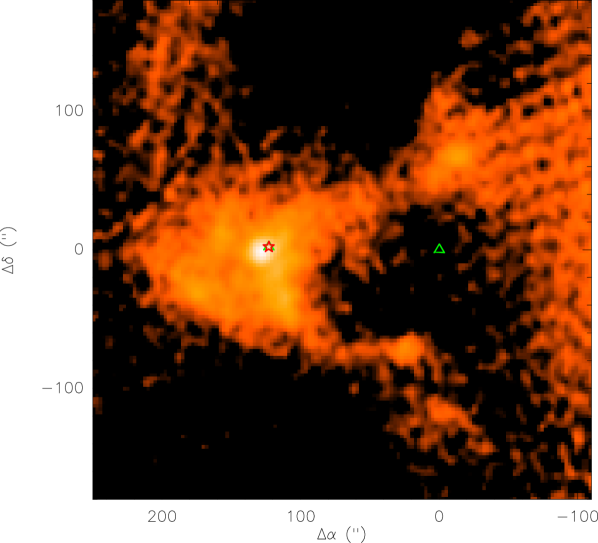
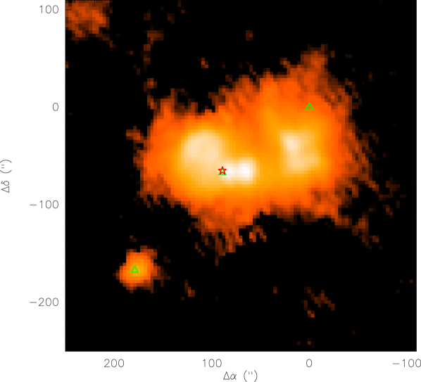
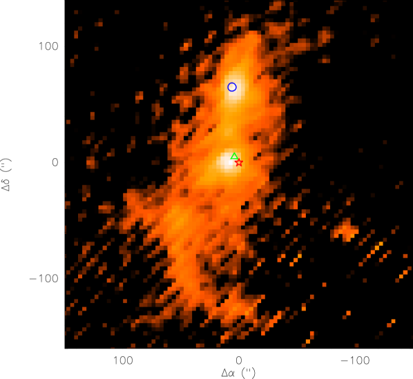
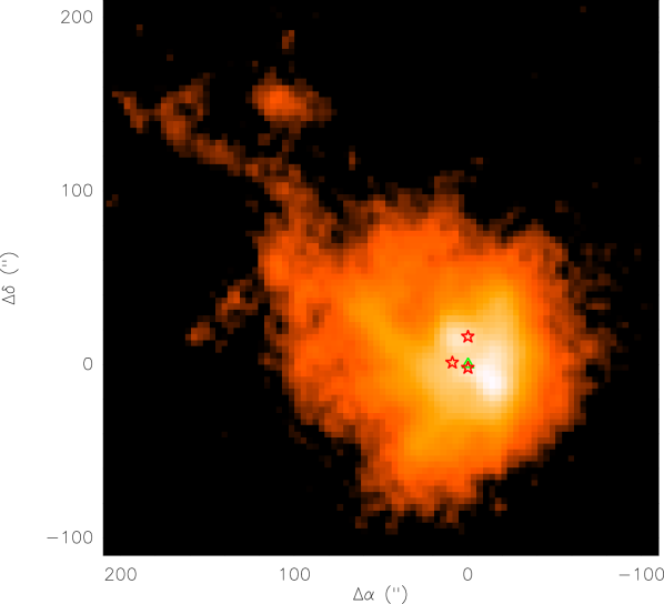
Figure 1: Maps of the sample sources in continuum at 1.2 mm obtained at the IRAM 30-m telescope. The sources are (from left to right and from top to bottom): S187, W3, S255 and S140. The intensity scale is logarithmic. The triangles mark water masers, the stars indicate point IR sources (IRAS point sources for S187, S255 and W3; IRS1, IRS2 and IRS3 for S140). The circle corresponds to the submillimetre source SMA1 in the S255 N clump area (Cyganowski, Brogan & Hunter, 2007).

Table 2: Results of the continuum observations: brightness ($B$), fluxes ($F$) and angular sizes ($\theta$) of the emission clumps towards selected positions.

Source	$\Delta\alpha$	$\Delta\delta$	$B$	$F$	$\theta$	Peak
	(′′)	(′′)	(Jy/beam)	(Jy)	(′′)
S 187	+160	0	0.15	2.1	45	CS
	0	+80	0.09	0.46	28	N2H+
W3	20	$-$40	2.03	19	38	CS
	+160	$-$160	0.70	2.23	22	N2H+
S 255	0	0	1.35	6.4	27	CS
	0	+60	1.24	6.4	28	N2H+
S 140	0	0	1.58	15.9	39	CS
	+40	+20	0.34	5.3	49	N2H+

3.1 Molecular maps and line parameters

3.1.1 S187

Maps of S187 in various lines overlaid on the greyscale map of the 1.2 mm continuum emission are presented in Fig. 2. The CS(2–1) and N₂H⁺(1–0) maps have been published earlier (Zinchenko et al., 1998; Pirogov et al., 2003). There is a striking difference between the various maps. Two separated clumps are clearly seen in N₂H⁺(1–0), which peaks North-West of the IRAS 01202+6133 source. The two peaks are still visible in the HNC(1–0) map, although they are not as well separated as in the N₂H⁺(1–0) map. All the other maps have a cometary or more irregular morphology, with peaks all shifted from the continuum peak. The gaussian line parameters at the CS and N₂H⁺ emission peaks are summarized in Table 3. In C¹⁸O $J=1-0$ and $J=2-1$ emission towards the CS peak there is an additional narrow ($\sim 0.7$ km/s) component at about $-$15.5 km/s. However, it is not pronounced in the lines of other high density tracers and we do not include it in Table 3.

The molecular data indicate the presence of at least 3 clumps in the area. There are several IRAS point sources and molecular masers here. The strongest IRAS point source, IRAS 01202+6133, is located at about 2′ to the east from our central position and coincides with the main 1.2 mm continuum peak. Here an OH maser and UC H ii region are present (Argon, Reid & Menten, 2000). The secondary N₂H⁺ peak coincides with this IRAS position. Also a weaker CS clump is located here as is clearly seen from the CS $J=5-4$ data. The main CS, HCO⁺ and HCN emission peaks are shifted by about 1′ further to the east. No IR sources or masers are known in this area. It is worth noting that the methanol emission peak is shifted still further to the east. At the same time C¹⁸O emission peaks near IRAS 01202+6133.

The strongest N₂H⁺ peak coincides with a relatively weak 1.2 mm continuum clump. It is shifted by about 0$\aas@@fstack{\prime}$5 from the strong near IR source NIRS 60 (Salas, Cruz-Gonzalez & Porras, 1998).

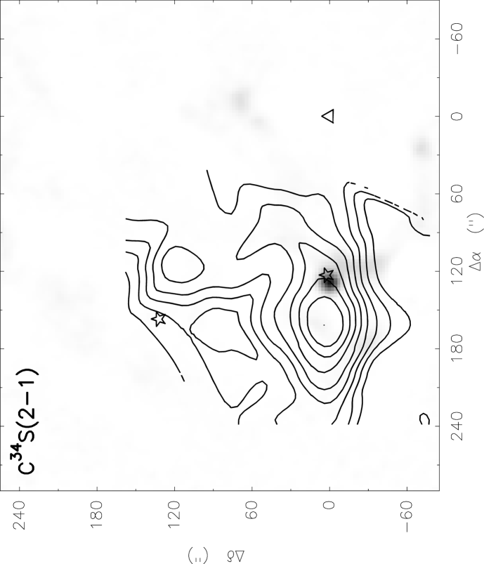
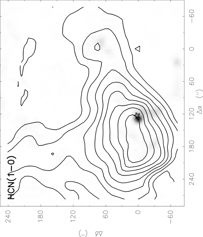
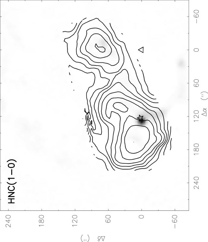
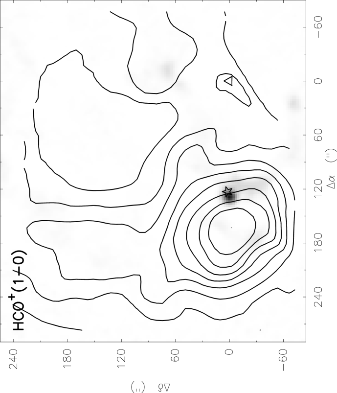
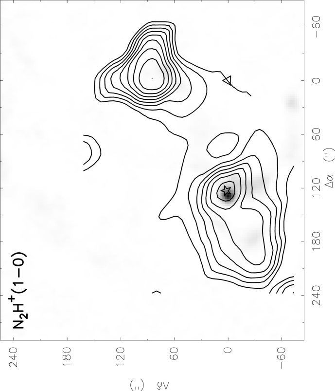
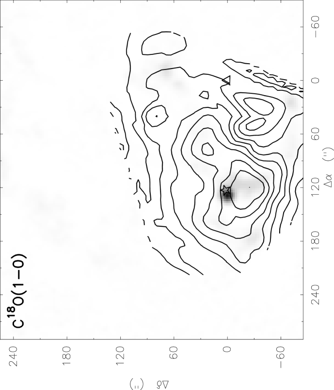
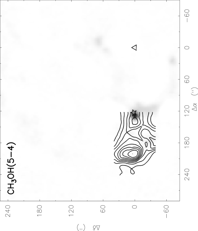
Figure 2: Maps of S187 in various molecular lines (contours) overlaid on the map of 1.2 mm dust continuum emission (grayscale). The contour levels span from 20% to 100% of the peak intensity in steps of 10%.

Table 3: Molecular line parameters at the CS and N₂H⁺ emission peaks in S187.

	(+160′′,0)				(0,+80′′)
Line	$T_{\rm mb}$	$V_{\rm LSR}$	$\Delta V$		$T_{\rm mb}$	$V_{\rm LSR}$	$\Delta V$
	(K)	(km/s)	(km/s)		(K)	(km/s)	(km/s)
C18O(1–0)	5.47(18)	$-$13.92(03)	1.71(09)		3.24(18)	$-$13.78(04)	1.67(10)
C18O(2–1)	5.85(19)	$-$14.05(02)	1.69(05)
CS(2–1)	4.29(10)	$-$14.26(03)	2.30(07)		1.20(20)	$-$13.63(27)	3.24(70)
C34S(2–1)	1.00(04)	$-$14.05(04)	2.25(11)
CS(5–4)	3.58(06)	$-$14.09(01)	1.86(03)
C34S(5–4)	$<$0.4
HCN(1–0)	5.14(07)	$-$14.31(02)	2.33(04)		1.92(08)	$-$13.81(04)	1.63(07)
H13CN(1–0)	0.50(05)	$-$14.17(10)	1.83(21)
HCO+(1–0)	5.54(08)	$-$14.49(02)	2.22(04)		2.41(08)	$-$14.03(03)	1.85(08)
H13CO+(1–0)	0.58(07)	$-$14.15(09)	1.56(22)		1.28(10)	$-$13.51(03)	0.83(07)
HNC(1–0)	5.44(12)	$-$14.29(02)	2.27(06)		5.70(15)	$-$13.58(02)	1.39(04)
HN13C(1–0)	0.33(04)	$-$13.88(09)	1.66(20)		0.63(05)	$-$13.35(03)	0.76(07)
N2H+(1–0)	0.61(08)	$-$14.09(07)	1.45(20)		1.59(12)	$-$13.33(03)	0.90(06)

3.1.2 W3

The molecular line maps of W3 are shown in Fig. 3 overlaid with the 1.2 mm continuum emission map. The CS(2–1) and N₂H⁺(1–0) maps have been published earlier (Zinchenko et al., 1998; Pirogov et al., 2003). The brightest continuum peak is attributed to free-free emission from a compact H ii region (e.g. Tieftrunk et al., 1997). There are two main molecular emission peaks in this area associated with two dust clumps. As in the S187 case, the N₂H⁺ map looks very different from most other maps. The N₂H⁺ peak coincides with a relatively weak south-east (SE) clump at the approximately (160^′′,$-$160^′′) position. The gaussian line parameters at the CS and N₂H⁺ emission peaks are summarized in Table 4. Some spectra clearly show non-gaussian features: broad wings at the CS peak position and red-shifted self-absorption in HCO⁺ at the N₂H⁺ peak.

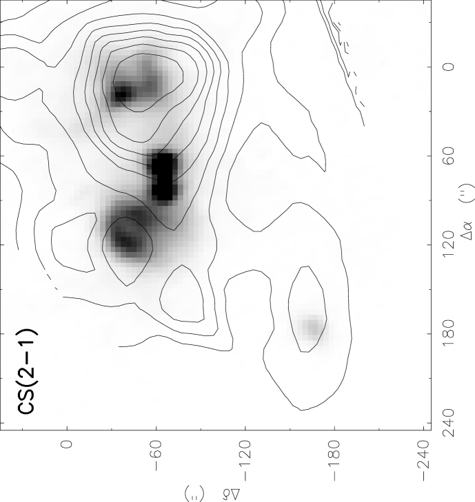
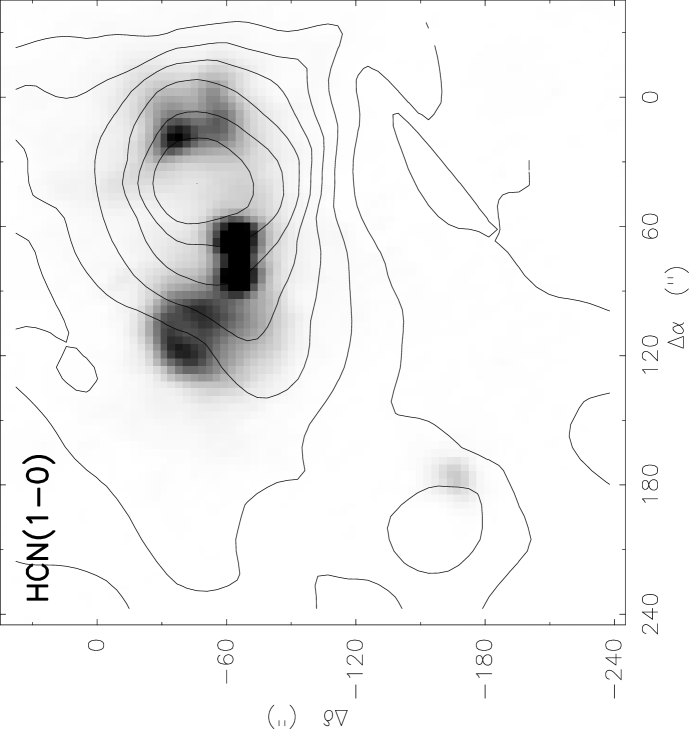
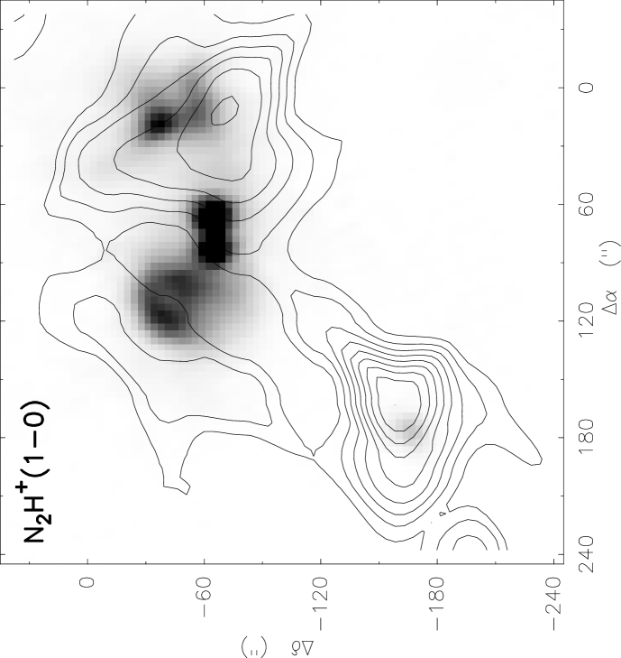
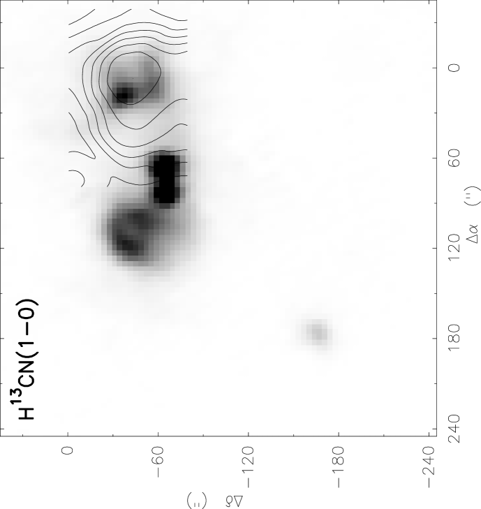
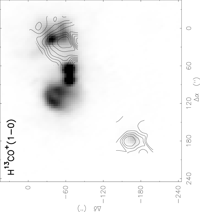
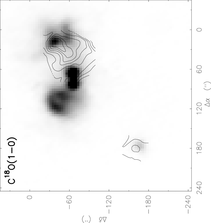
Figure 3: Maps of W3 in various molecular lines (contours) overlaid on the map of 1.2 mm continuum emission (grayscale). The contour levels span from 20% to 100% of the peak intensity in steps of 10%.

Table 4: Molecular line parameters at the CS and N₂H⁺ emission peaks in W3.

	(0,$-$40′′)				(+160′′,$-$160′′)
Line	$T_{\rm mb}$	$V_{\rm LSR}$	$\Delta V$		$T_{\rm mb}$	$V_{\rm LSR}$	$\Delta V$
	(K)	(km/s)	(km/s)		(K)	(km/s)	(km/s)
C18O(1–0)	2.05(20)	$-$42.70(27)	5.32(71)		2.36(37)	$-$38.58(11)	1.49(27)
CS(2–1)	8.82(10)	$-$43.09(03)	4.76(06)		3.19(03)	$-$38.66(19)	4.43(53)
HCN(1–0)	7.96(11)	$-$43.08(02)	3.41(05)		1.65(13)	$-$38.55(40)	8.08(38)
H13CN(1–0)	1.51(07)	$-$42.75(12)	4.62(20)
HCO+(1–0)	16.26(07)	$-$43.40(01)	3.86(02)		4.05(06)	$-$38.97(04)	4.73(09)
H13CO+(1–0)	0.88(17)	$-$43.11(21)	2.44(51)		0.95(18)	$-$38.33(19)	2.02(45)
HNC(1–0)	5.36(11)	$-$42.92(04)	3.83(09)		4.41(12)	$-$38.74(04)	3.12(10)
HN13C(1–0)	0.37(03)	$-$42.63(09)	2.80(21)		0.17(01)	$-$38.38(05)	2.95(23)
N2H+(1–0)	0.66(09)	$-$42.22(11)	2.04(30)		1.37(10)	$-$38.76(10)	1.75(14)

3.1.3 S255

For S255 we have the most complete data set. In addition to the common set of molecular transitions it includes SO($3_{2}-2_{1}$), SiO (2–1) and (5–4), several methanol 2–1 and 5–4 series lines. Earlier we mapped it also in ammomia (1,1) and (2,2) (Zinchenko, Henning & Schreyer, 1997). The molecular maps overlaid on the greyscale map of the 1.2 mm continuum emission are presented in Fig. 4. This source was mapped at 1.2 mm in continuum at the IRAM 30m telescope by Mezger et al. (1988). Our observations with the new array receiver provide a better sensitivity and a wider map area, although the basic features of our map are consistent with those previous results.

The maps show two main peaks of molecular and dust continuum emission, around the (0,0) and (0,+60^′′) positions. The commonly accepted names for these clumps are S255IR and S255N. There is also a third (southern) peak at about (+20^′′,$-$50^′′) noticeable in the continuum map and in several molecular maps, at least in N₂H⁺(1–0) and HCO⁺(1–0). N₂H⁺ and ammonia are significantly stronger at the northern peak (S255N) while most other species are either stronger at the central position (S255IR) or comparable at both central and northern clumps. The dust emission is almost equal for these clumps. The nature of these two components is different. The central one is associated with a luminous cluster of IR sources, whereas toward the northern one an ultracompact H ii region (G192.58-0.04) was detected. Recently several compact submillimetre continuum clumps were detected there with SMA (Cyganowski et al., 2007). This object is extremely red in the mid-IR band (Crowther & Conti, 2003). Mezger et al. (1988) derived almost exactly the same dust masses and temperatures for both components from their 1.2 mm and $350\mu$m observations. The gaussian line parameters at the central and northern emission peaks are summarized in Table 5.

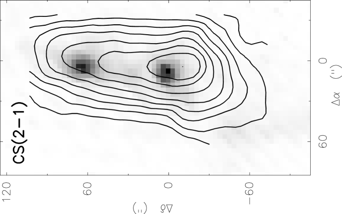
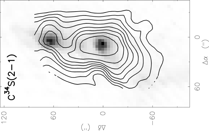
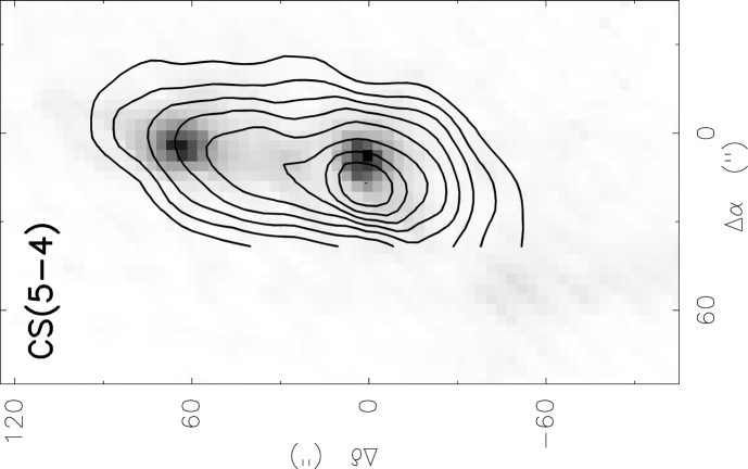
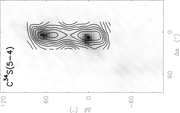
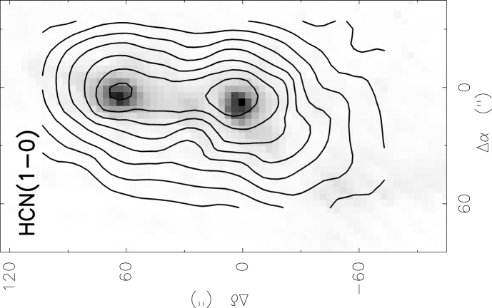
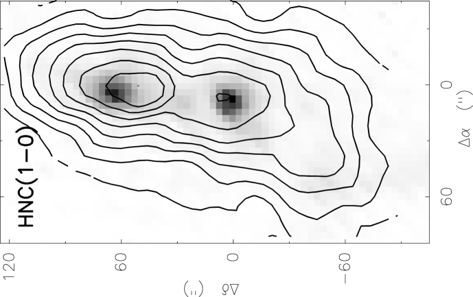
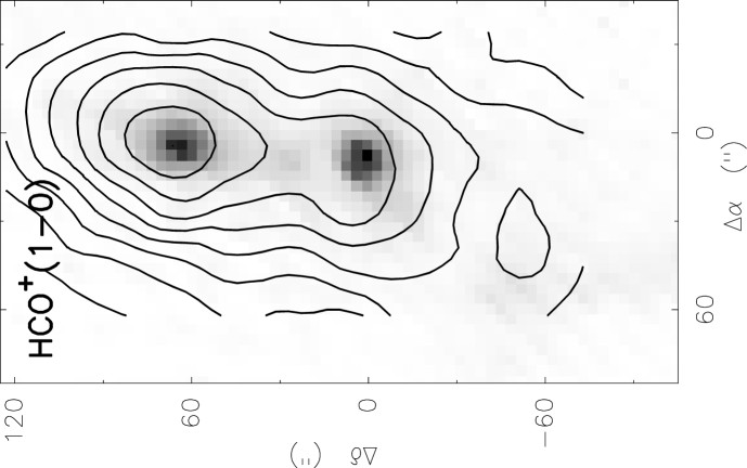
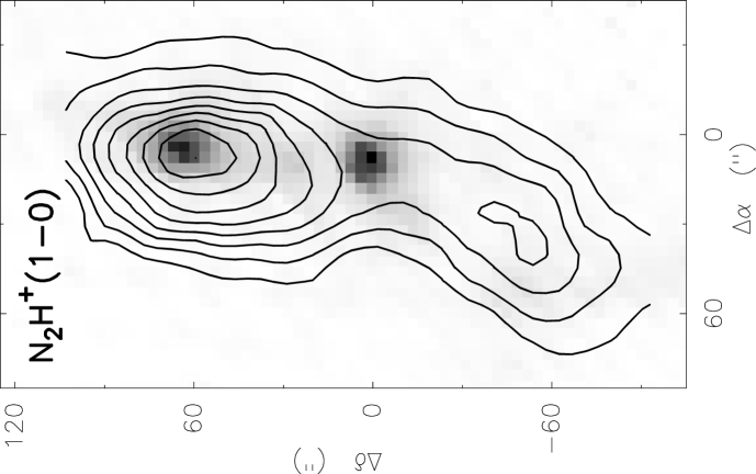
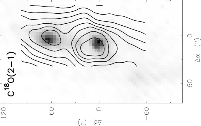
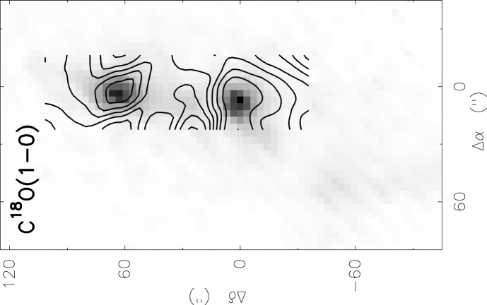
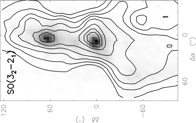
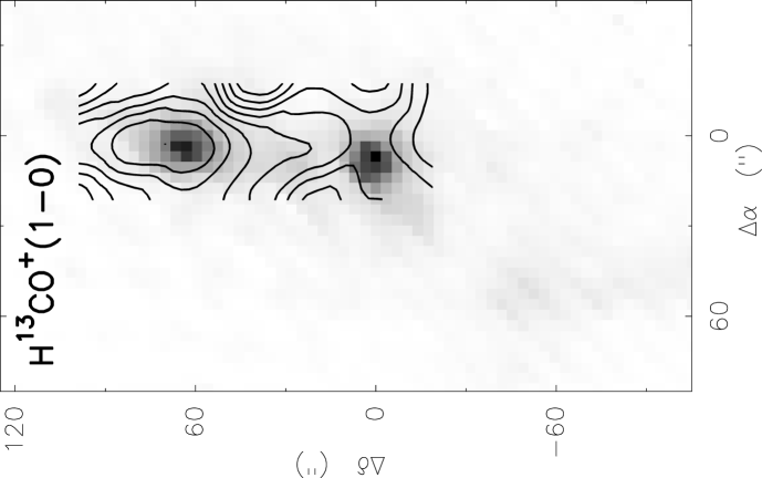
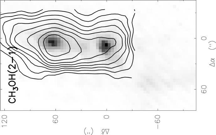
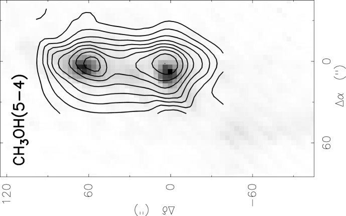
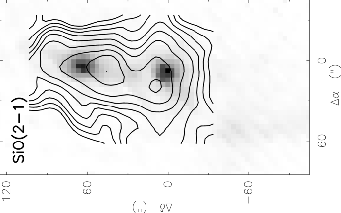
Figure 4: Maps of S255 in various molecular lines (contours) overlaid on the map of 1.2 mm dust continuum emission (grayscale). The contour levels span from 20% to 100% of the peak intensity in steps of 10%.

Table 5: Molecular line parameters at the CS (central) and N₂H⁺ (northern) emission peaks in S255.

	(0,0)				(0,+60′′)
Line	$T_{\rm mb}$	$V_{\rm LSR}$	$\Delta V$		$T_{\rm mb}$	$V_{\rm LSR}$	$\Delta V$
	(K)	(km/s)	(km/s)		(K)	(km/s)	(km/s)
C18O(1–0)	1.99(12)	6.84(17)	4.31(43)		1.67(13)	8.74(14)	3.71(34)
C18O(2–1)	6.45(08)	7.18(01)	2.88(03)		5.89(08)	8.82(01)	2.95(03)
CS(2–1)	13.36(09)	7.46(01)	2.78(02)		9.08(08)	8.40(01)	3.16(03)
C34S(2–1)	1.93(11)	7.46(08)	2.78(18)		1.33(10)	8.56(12)	3.20(29)
CS(5–4)	10.94(12)	7.49(01)	2.73(03)		7.46(12)	8.55(02)	3.32(05)
C34S(5–4)	1.13(06)	7.52(05)	2.33(12)		0.75(08)	9.10(13)	3.57(26)
HCN(1–0)	13.79(11)	7.33(01)	3.25(03)		11.52(11)	8.40(02)	3.60(03)
H13CN(1–0)	1.41(07)	7.57(06)	2.58(12)		1.37(07)	8.91(06)	2.12(11)
HCO+(1–0)	7.34(10)	7.53(03)	3.90(06)		11.27(11)	8.83(02)	3.21(04)
H13CO+(1–0)	0.74(10)	7.51(11)	1.69(26)		1.39(08)	8.97(07)	2.79(18)
HNC(1–0)	11.87(18)	7.30(02)	2.73(05)		11.30(17)	8.55(02)	3.32(06)
HN13C(1–0)	0.18(02)	7.29(20)	3.30(47)		0.28(02)	8.87(16)	4.78(37)
N2H+(1–0)	1.46(06)	7.44(04)	2.25(10)		2.58(05)	8.97(02)	2.61(06)
SiO(2–1)	0.18(06)	7.96(52)	3.32(122)		0.20(05)	8.06(61)	5.24(144)

3.1.4 DR-21 NH₃

This is another well known site of active star formation. The CS, HCN and HCO⁺ spectra here suffer from a very strong red-shifted self-absorption (Fig. 5), which makes an analysis of corresponding maps almost senseless. For this reason we present here and discuss only rarer isotopologue and N₂H⁺(1–0) maps (Fig. 6). We did not map the dust continuum emission in this area, given that it has been already observed by Chandler, Gear & Chini (1993). It is easy to see that the N₂H⁺ and HN¹³C peaks are shifted by about 0$\aas@@fstack{\prime}$5 to the south from the emission peaks of other species. The latter peaks practically coincide with the main dust emission peak DR21(OH)M in the notation introduced by Mangum, Wootten & Mundy (1991). The N₂H⁺ and HN¹³C peaks lie near a weaker dust peak DR21(OH)S. The gaussian line parameters are given in Table 6.

Figure 5: Molecular line spectra towards the N₂H⁺ emission peak in DR-21 NH₃.

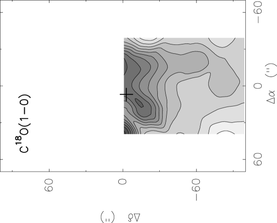
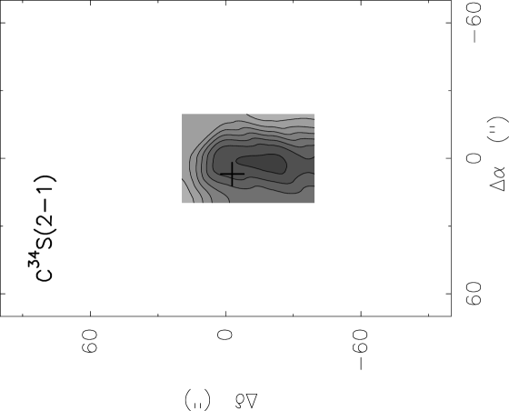
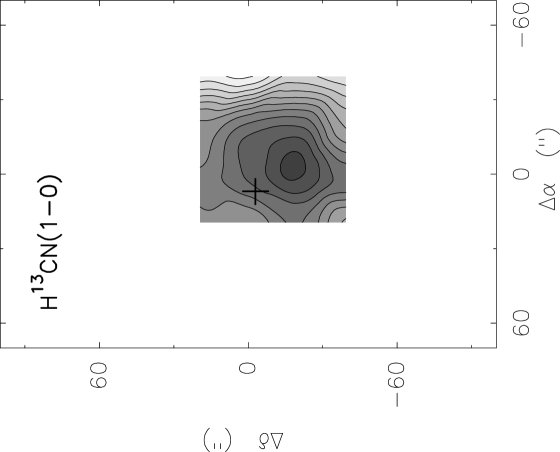
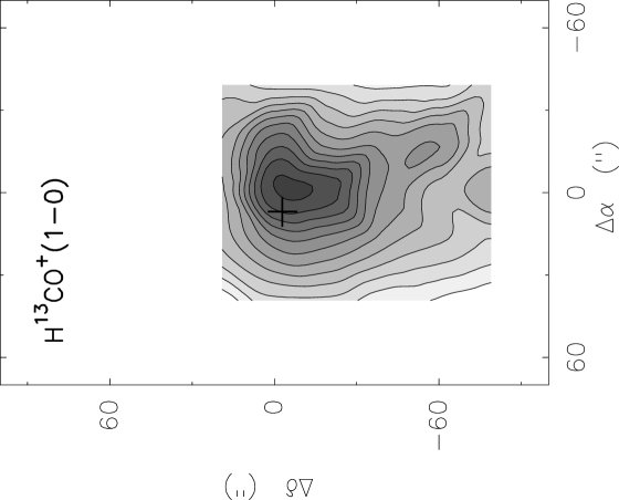
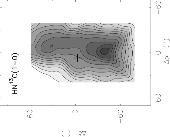
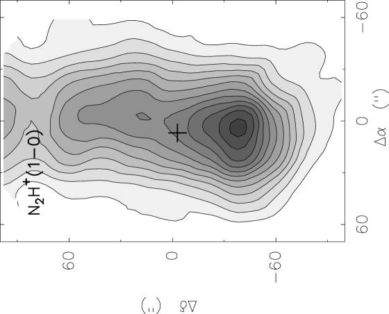
Figure 6: Maps of DR-21 NH₃ in various molecular lines. The contour levels span from 20% to 100% of the peak intensity in steps of 10%. The cross marks the position of DR21 (OH).

Table 6: Molecular line parameters at the CS and N₂H⁺ emission peaks in DR-21 NH₃.

	(0,$-$20′′)				(0,$-$40′′)
Line	$T_{\rm mb}$	$V_{\rm LSR}$	$\Delta V$		$T_{\rm mb}$	$V_{\rm LSR}$	$\Delta V$
	(K)	(km/s)	(km/s)		(K)	(km/s)	(km/s)
C18O(1–0)	4.99(14)	$-$2.99(05)	3.84(13)		4.69(15)	$-$3.37(05)	3.28(12)
C34S(2–1)	2.62(06)	$-$3.04(05)	4.68(12)		2.89(06)	$-$3.01(04)	3.83(10)
H13CN(1–0)	2.34(06)	$-$3.24(06)	4.07(10)		2.34(06)	$-$3.47(05)	3.58(09)
H13CO+(1–0)	3.17(07)	$-$3.46(04)	3.67(09)		2.73(07)	$-$3.57(04)	3.25(10)
HN13C(1–0)	1.34(09)	$-$3.05(14)	4.38(32)		1.70(09)	$-$3.25(10)	3.56(23)
N2H+(1–0)	4.99(04)	$-$3.11(02)	4.04(03)		6.93(04)	$-$3.25(01)	3.51(02)

3.1.5 S140

S140 is one of the best studied sites of active star formation. In particular it was observed at various instruments in the HCN, HCO⁺ and CO isotopic lines (e.g. Park & Minh, 1995). Nevertheless, we present here our own data on these lines too, to better compare with other molecular maps (all maps have been obtained at Onsala). The N₂H⁺ results have been published earlier (Pirogov et al., 2003).

The maps (Fig. 7) clearly show that HCN and HCO⁺ emissions peak near the (0,0) position while the N₂H⁺ peak is shifted to about (+50^′′,+20^′′). A multi-transitional CS study (Zhou et al., 1994) shows that CS emission peak is near the (0,0) position. HNC is an intermediate case and there is a secondary HNC peak near the N₂H⁺ peak. These differences in emission distributions are not caused by opacity effects because the maps in the lines of rarer isotopic modifications of these molecules show the same features (the N₂H⁺ optical depth is rather small, $\sim 0.4$, as shown by Pirogov et al. 2003). The gaussian line parameters are presented in Table 7.

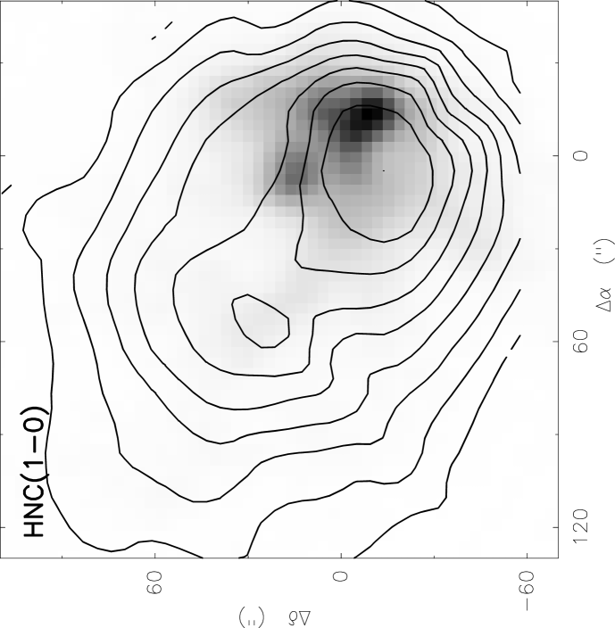
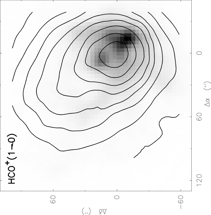
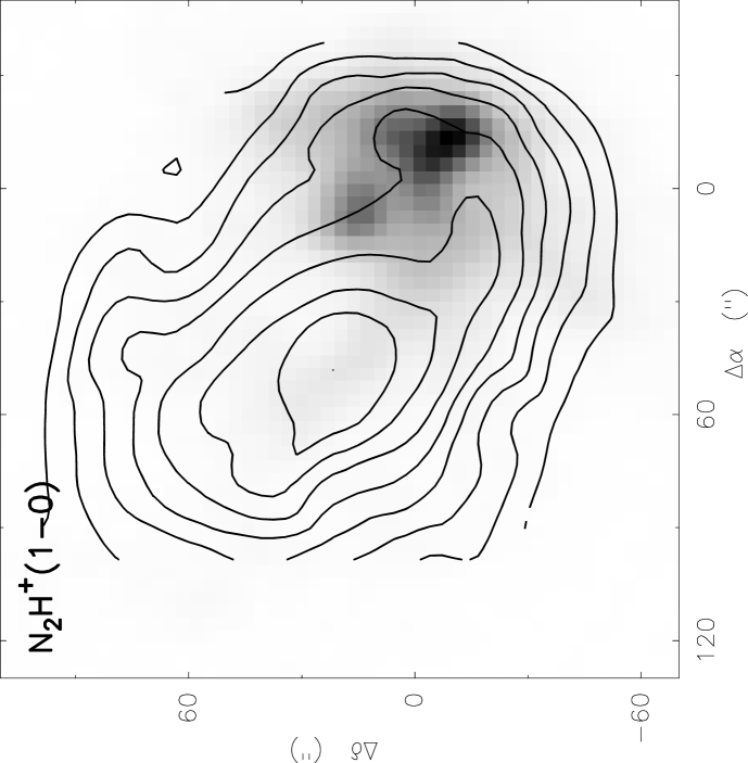
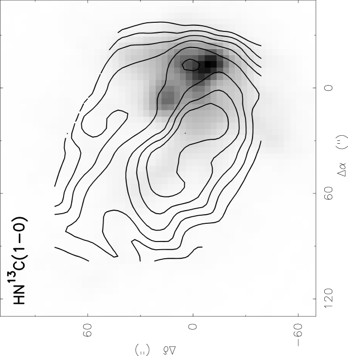
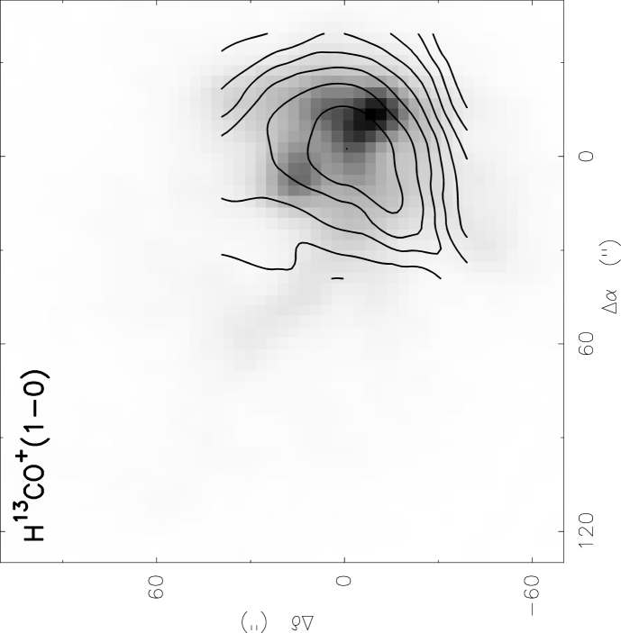
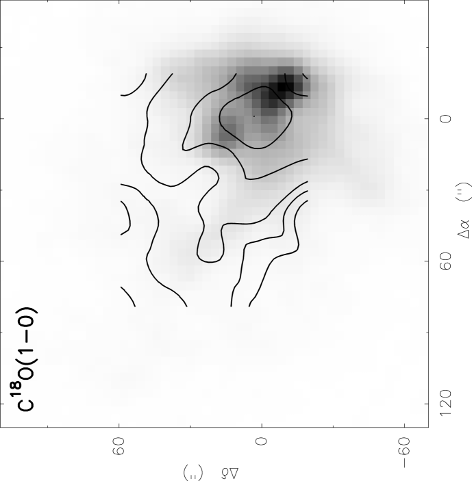
Figure 7: Maps of S140 in various molecular lines (contours) overlaid on the map of 1.2 mm dust continuum emission (grayscale). The contour levels span from 20% to 100% of the peak intensity in steps of 10%.

Table 7: Molecular line parameters at the CS and N₂H⁺ emission peaks in S140.

	(0,0)				(+40′′,+20′′)
Line	$T_{\rm mb}$	$V_{\rm LSR}$	$\Delta V$		$T_{\rm mb}$	$V_{\rm LSR}$	$\Delta V$
	(K)	(km/s)	(km/s)		(K)	(km/s)	(km/s)
C18O(1–0)	3.19(16)	$-$6.83(09)	3.46(22)		2.53(18)	$-$7.51(10)	2.95(24)
HCN(1–0)	18.37(11)	$-$6.80(01)	3.05(02)		11.43(11)	$-$6.92(01)	2.84(03)
H13CN(1–0)	1.50(07)	$-$7.00(05)	2.22(10)		0.79(08)	$-$6.96(08)	1.53(16)
HCO+(1–0)	25.63(09)	$-$6.91(01)	3.05(01)		15.13(09)	$-$6.88(01)	2.86(02)
H13CO+(1–0)	2.64(10)	$-$7.18(05)	2.58(11)		1.94(10)	$-$7.21(06)	2.26(14)
HNC(1–0)	16.62(17)	$-$6.77(01)	2.83(03)		14.95(18)	$-$7.03(02)	2.51(04)
HN13C(1–0)	0.68(05)	$-$6.42(12)	3.27(27)		1.24(07)	$-$6.94(05)	1.75(11)
N2H+(1–0)	3.41(07)	$-$6.90(02)	2.20(05)		6.33(09)	$-$7.00(01)	1.87(03)

4 Physical parameters of the sources and molecular abundances

4.1 Kinetic temperatures

The kinetic temperatures of the sources have been estimated from the CH₃C₂H observations. As shown e.g. by Bergin et al. (1994) this symmetric-top molecule is a good “thermometer” for gas densities $n\ga 10^{4}$ cm^-3. Our main goal is to compare the temperatures at the peaks of the CS and N₂H⁺ emission. At first, we derived the temperatures from the CH₃C₂H $J=6-5$ data obtained at Onsala. These measurements were done only at the peak positions. Later the CH₃C₂H $J=13-12$ emission was mapped at IRAM with the multibeam receiver. The details of the temperature estimates are published elsewhere (Malafeev et al., 2005, Zinchenko et al., in preparation). Here we present the main results. In S187 the CH₃C₂H emission was too weak.

The kinetic temperatures at the CS and N₂H⁺ peaks, derived from the Onsala and IRAM CH₃C₂H data, are listed in Table 8. It is easy to see that in most cases there is no significant temperature difference between the CS and N₂H⁺ emission peaks, although on average the N₂H⁺ peaks are somewhat colder than the CS ones.

Table 8: Kinetic temperatures at the CS and N₂H⁺ peaks derived from the Onsala and IRAM CH₃C₂H data ($T_{\rm kin}^{6-5}$ and $T_{\rm kin}^{13-12}$, respectively).

Source	$\Delta\alpha$	$\Delta\delta$	$T_{\rm kin}^{6-5}$	$T_{\rm kin}^{13-12}$	Emission
	$(^{\prime\prime})$	$(^{\prime\prime})$	(K)	(K)	peak
W3	20	-40	$52.6\pm 3.1$	$58.4\pm 1.5$	CS
	160	-160	$30.7\pm 0.8$	$37.3\pm 2.2$	N2H+
S255	0	60	$34.9\pm 1.4$	$39.6\pm 0.4$	N2H+
	0	0	$34.5\pm 1.0$	$38.8\pm 0.9$	CS
DR21	0	-40	$28.8\pm 0.1$	$34.8\pm 1.1$	N2H+
	0	0	$33.4\pm 2.7$	$44.0\pm 1.4$	CS
S140	40	20	$27.8\pm 1.6$	$37.7\pm 2.2$	N2H+
	0	0	$30.6\pm 0.7$	$42.4\pm 1.0$	CS

CH₃C₂H maps of sufficiently high quality were obtained at IRAM for DR21, S140 and the CS peak in W3. The IRAM data indicate somewhat higher peak temperatures than obtained from the Onsala data, as expected due to a higher angular resolution and higher excitation requirements for the $J=13-12$ transition if temperature increases towards an embedded heating source. Our data do show such temperature gradients consistent with theoretical expectations (Zinchenko et al., 2005) but we do not discuss them here. At the same time the IRAM data confirm our main conclusion that there is no significant temperature difference between the CS and N₂H⁺ peaks in most cases, although the N₂H⁺ peaks are somewhat colder than the CS ones, on average.

It is interesting to compare our estimates of kinetic temperature with other available data for these sources. Most of them have been actively studied. Such comparison was made by Malafeev et al. (2005) and here we repeat the main points.

4.1.1 W3

Based on NH₃(1,1) and (2,2) lines, Tieftrunk et al. (1998) derived kinetic temperatures of 44 K and 25 K toward our CS and N2H+ peaks, respectively. A comparison with Table 8 shows that these temperatures are somewhat lower than those obtained from the CH₃C₂H data, although the relation is the same.

4.1.2 S255

From our ammonia observations (Zinchenko et al., 1997) the kinetic temperature at the (0,+80^′′) position (near the NH₃ and N₂H⁺ peaks) is $23\pm 1$ K. At the central position the uncertainty in the kinetic temperature is too high. Schreyer et al. (2000) obtained the kinetic temperature in the centre from their ammonia data of 30.8 K and the dust temperature from the IRAS data of 31.1 K. Mezger et al. (1988) derived almost the same dust temperatures ($\sim 30$ K) for the two peaks discussed here from their 1.3 mm and 350 $\mu$m continuum observations.

4.1.3 DR21 NH₃

This source was observed (without mapping) in the CH₃C₂H lines at the 11-m NRAO telescope (Kuiper et al., 1984). They observed the same $J=6-5$ transition and derived practically the same kinetic temperature at the centre as in our present work, 33.0 K. There are VLA ammonia observations by Mangum, Wootten & Mundy (1992). They derived kinetic temperatures of 32 K at the (0,0) position and 25 K near the (0,$-$40^′′) position. This is rather close to our estimates.

4.1.4 S140

S140 was also observed in CH₃C₂H at the 11-m NRAO telescope by Kuiper et al. (1984). They obtained for the cloud centre the kinetic temperature of $32.1\pm 6.7$ K which coincides with our $J=6-5$ estimate within the uncertainties. From ammonia observations at Effelsberg, Ungerechts, Walmsley & Winnewisser (1986) found a temperature of about 20 K, once again a value significantly lower than found with CH₃C₂H. The dust temperature from IRAS data is 34 K (Zhou et al., 1994), more similar to our findings. Thus, CH₃C₂H appears to better trace the dust.

4.2 Masses and densities

There are several ways to estimate masses and densities of interstellar clouds. Here we derive the source masses and column densities primarily from the dust continuum observations. This is considered to be one of the most reliable methods, partly due to the fact that dust/gas mass ratio is rather constant. At the same time the uncertainties in the dust opacities are still rather high. Additional uncertainties are related to uncertainties in the dust temperature. Here we use the temperature estimates obtained from our methyl acetylene observations, found to be similar to the dust temperature. It is known that at the typical densities of dense cores the dust and gas kinetic temperatures are close to each other. The results of these estimates are presented in Table 9. It is worth noting that the masses here are not really total masses of the sources because they are derived from the fluxes integrated over 1′ diameter circle around the indicated positions. The dust opacities were adopted from Ossenkopf & Henning (1994). The gas/dust mass ratio was assumed to be equal to 100. In addition we present also estimates of the average volume density along the line of sight obtained as $\bar{n}=N_{\rm L}/L$ where the size $L$ is derived from the angular size (Table 2) and distance to the source (Table 1).

In the last column we give estimates of the virial masses of the clumps based on these sizes and widths of optically thin lines at these positions. These estimates are rather uncertain, at least by a factor of 2 due to large uncertainties in the parameters. Nevertheless, within this factor they agree well with the masses derived from continuum observations. This shows that the clumps are close to gravitational equilibrium.

Table 9: Estimates of the gas column densities, average volume densities and masses from the continuum observations. In the last column estimates of the virial masses are given.

Source	Peak	$N_{\rm L}\times 10^{-23}$	$\bar{n}\times 10^{-5}$	$M$	$M_{\mathrm{vir}}$
		(cm-2)	(cm-3)	(M☉)	(M☉)
S 187	CS	0.4	0.7	30	50
	N2H+	0.5	1.0	14	10
W3	CS	2.0	1.6	405	310
	N2H+	1.2	1.5	74	90
S 255	CS	2.0	1.9	290	210
	N2H+	1.9	1.6	280	220
S 140	CS	2.8	3.9	86	90
	N2H+	0.6	0.7	32	70

The average gas volume densities are $\bar{n}\sim 10^{5}$ cm^-3 in all cases. However, it is well known that such mean densities can be significantly lower than densities found from molecular excitation analysis (e.g. Zinchenko et al., 1998). This discrepancy is most probably explained by small-scale gas clumpiness. Such clumpiness is indicated by many studies (e.g. Bergin, Snell & Goldsmith, 1996). At the same time our data do not provide sufficient material for excitation analysis in most cases. Only for S255 we have 3 mm and 1.3 mm data in C¹⁸O, CS, C³⁴S and methanol transitions towards both CS and N₂H⁺ peaks which can be used for modeling. In particular, our LVG estimates of gas density from the C³⁴S data give values of about $n\sim 5\times 10^{5}$ cm^-3 for both components. Methanol data modeling gives $n\sim 3\times 10^{5}$ cm^-3 also for both peaks (S. Salii, private communication). Estimates based on C¹⁸O are highly uncertain but are consistent with these values and show similar densities for both components because the line intensity ratios are similar. These estimates are rather close to the average densities presented in Table 9, although somewhat higher as expected. This shows that the volume filling factor in this density range is rather high. The continuum data also indicate practically equal mean gas densities for the components.

4.3 Abundances

We derive here abundances of several species which were observed in all our sources and are the most informative ones for our purposes: C¹⁸O, H¹³CN, H¹³CO⁺, HN¹³C, N₂H⁺ and C³⁴S. In most cases we use only rare isotope data which are presumably not affected by optical depth effects. The optical depth in the N₂H⁺ lines is also small or moderate as shown by Pirogov et al. (2003). The column densities are estimated from integrated line intensities in the LTE approximation assuming the excitation temperatures equal to the kinetic temperatures as given in Table 8 (approximate values close to $T_{\rm kin}^{6-5}$ and $T_{\rm kin}^{13-12}$ were used). For S187 we assume $T_{\rm kin}$ of 20 K for the CS peak and $T_{\rm kin}$ of 10 K for the N₂H⁺ peak (taking into account narrow line widths and very weak CH₃C₂H emission). Then, we derive abundances from comparison of the molecular column densities and total gas column densities obtained from dust continuum observations (Table 9). In order to take into account different beam sizes we correct the abundance estimates assuming Gaussian beams and Gaussian brightness distributions. For DR21 where we do not have our own dust continuum data, the abundances were derived assuming $X(\mathrm{C^{18}O})=2\times 10^{-7}$. The results are summarized in Table 10. Pirogov et al. (2003) derived N₂H⁺ abundances in a different way: from the N₂H⁺ column densities and virial masses of the clouds. Nevertheless, their estimates are very close to those presented in Table 10 when the positions coincide (within a factor of 2).

Table 10: Estimates of molecular and electron abundances towards selected positions in the sample sources. For C¹⁸O, abundances derived from the $J=1-0$ and $J=2-1$ transitions are shown separately.

Source	$\Delta\alpha$	$\Delta\delta$	$X$(C18O)10	$X$(C18O)21	$X$(H13CN)	$X$(H13CO+)	$X$(HN13C)	$X$(C34S)	$X$(N2H+)	$X_{\mathrm{e}}$
	$(^{\prime\prime})$	$(^{\prime\prime})$
S187	160	0	4.2E$-$07	1.5E$-$07	1.0E$-$10	5.8E$-$11	6.5E$-$11	6.0E$-$10	6.5E-11	1.7E-07
	0	80	2.5E$-$07			7.6E$-$11	6.2E$-$11		1.2E-10	1.3E-07
W3	0	$-$40	2.9E$-$07		4.8E$-$10	8.6E$-$11	7.6E$-$11		6.5E-11	1.2E-07
	160	$-$160	2.0E$-$07			1.9E$-$10	8.8E$-$11		2.7E-10	5.4E-08
S255	0	0	2.4E$-$07	1.4E$-$07	2.8E$-$10	5.7E$-$11	4.9E$-$11	9.2E$-$10	1.7E-10	1.8E-07
	0	60	1.8E$-$07	1.3E$-$07	2.3E$-$10	1.9E$-$10	1.2E$-$10	7.7E$-$10	3.7E-10	5.4E-08
DR21	0	$-$20			2.2E$-$10	1.6E$-$10	1.5E$-$10	6.3E$-$10	3.2E-10	6.3E-08
	0	$-$40			2.4E$-$10	1.5E$-$10	1.9E$-$10	7.2E$-$10	4.7E-10	6.7E-08
S140	0	0	1.3E$-$07		1.0E$-$10	1.2E$-$10	7.1E$-$11		1.5E-10	8.4E-08
	40	20	3.4E$-$07		1.4E$-$10	2.9E$-$10	2.7E$-$10		9.1E-10	3.4E-08

Non-LTE modeling for some clumps in our sample using the LVG approximation or the RADEX code (based on the escape probability method; van der Tak et al. 2007) gives systematically lower (by a factor of 1.5–2) column densities for all species considered here, except C¹⁸O, assuming temperature and density as described above. This is a natural result because C¹⁸O is practically thermalized at these conditions while the other species are still far from equilibrium and population of lower levels exceeds that expected in LTE. Nevertheless, we believe that non-LTE modeling is not justified here due to the absence of the necessary data for most of the sources. One can bear in mind that the abundances derived here are somewhat overestimated.

4.4 Ionization fraction

The ionization fraction can be estimated from the HCO⁺ abundance using the results of relevant chemical models. It is known that in dense clouds HCO⁺ is formed mainly from H${}_{3}^{+}$ (e.g. Turner, 1995):

$$\mathrm{H_{3}^{+}}+\mathrm{CO}\rightarrow\mathrm{HCO^{+}}+\mathrm{H_{2}}$$ (1)

and is destroyed by dissociative recombination:

$$\mathrm{HCO^{+}}+e\rightarrow\mathrm{CO}+\mathrm{H}$$ (2)

In addition, one has to take into account HCO⁺ recombination onto negatively charged dust grains (e.g. Caselli et al., 2008). The rate of this reaction is given by the product $k_{\mathrm{g}}X_{\mathrm{g}}$ where the rate coefficient $k_{\mathrm{g}}$ and the fractional abundance of dust grains $X_{\mathrm{g}}$ are determined by grain size distribution and gas kinetic temperature (Draine & Sutin, 1987). For the typical temperatures in our objects ($\sim 30$ K) and MRN (Mathis et al., 1977) grain size distribution $k_{\mathrm{g}}X_{\mathrm{g}}\approx 3\times 10^{-15}$ s^-1.

In this model for HCO⁺ abundance in steady state we can write:

$$X(\mathrm{HCO^{+}})=\frac{k_{1}X(\mathrm{H_{3}^{+}})X(\mathrm{CO})}{\alpha(\mathrm{HCO^{+}})X_{e}+k_{\mathrm{g}}X_{\mathrm{g}}}$$ (3)

where $k_{1}$ is the rate of reaction (1) and $\alpha(\mathrm{HCO^{+}})$ is the HCO⁺ dissociative recombination rate.

H${}_{3}^{+}$ is formed by cosmic-ray ionization of molecular hydrogen and is destroyed in dense clouds primarily by reaction (1) (e.g. Black, 2000). For regions where CO is not frozen onto dust grains, recombination onto negatively charged grains is a negligible H${}_{3}^{+}$ destruction process compared with this reaction. Therefore, for H${}_{3}^{+}$ abundance in this regime we obtain:

$$X(\mathrm{H_{3}^{+}})=\frac{\zeta/n}{k_{1}X(\mathrm{CO})}$$ (4)

where $\zeta$ is the cosmic-ray ionization rate and $n$ is the total gas density. Now combining Eq. (3) and (4) we come to the following simple expression:

$$X(\mathrm{HCO^{+}})=\frac{\zeta/n}{\alpha(\mathrm{HCO^{+}})X_{e}+k_{\mathrm{g}}X_{\mathrm{g}}}$$ (5)

Estimates of the electron abundances based on this formula are presented in the last column of Table 10. The cosmic-ray ionization rate was assumed to be equal to $\zeta=3\times 10^{-17}$ s^-1, $\alpha(\mathrm{HCO^{+}})=7.5\times 10^{-7}$ s^-1cm³ (Turner, 1995). The gas density was assumed to be $n=10^{5}$ cm^-3 and $[\mathrm{HCO^{+}}]/[\mathrm{H^{13}CO^{+}}]=40$. The $k_{\mathrm{g}}X_{\mathrm{g}}$ term leads to corrections less than 10% in the $X_{\mathrm{e}}$ values and we neglected it. Strictly speaking, in this way we derive more reliably the parameter $nX_{\mathrm{e}}$, i.e. the electron density, not abundance. However, for a better comparison with other results we will discuss further mainly the $X_{\mathrm{e}}$ values.

5 Discussion

5.1 Variations of molecular abundances

An inspection of the observational results and estimates of the physical parameters presented above leads to several important conclusions:

(1) There are strong variations of the relative intensities in the lines of different molecular tracers across the investigated high mass star forming regions. In Paper I we mentioned already striking differences between N₂H⁺ and CS maps and the fact that the CS distribution follows that of the dust emission while N₂H⁺ does not. Now we see that C¹⁸O and HCN, like CS, are good tracers of the dust emission which presumably shows the total mass distribution. At the same time the behavior of HCO⁺ and HNC resembles that of N₂H⁺. Significant differences in distributions of various species in particular sources have been noticed in some other studies (e.g. Ungerechts et al., 1997) but here we see systematic effects common for the sources in the sample.

(2) There is no sign of CO and/or CS depletion in these objects (in contrast to cold dark clouds). The abundances derived for C¹⁸O from the $J=1-0$ and $J=2-1$ transitions more or less agree with each other. They are practically constant within each source and among the whole sample (with small deviations which can be caused e.g. by temperature uncertainties) and are close to the “canonical” values derived earlier (e.g. $X(\mathrm{C^{18}O})\approx 1.7\times 10^{-7}$ obtained by Frerking, Langer & Wilson 1982).

(3) The N₂H⁺ and HNC abundances significantly decrease with increasing ionization fraction (Fig. 8). The best fit gives $X(\mathrm{N_{2}H^{+}})\propto X_{\mathrm{e}}^{-1.3\pm 0.3}$ and $X(\mathrm{HN^{13}C})\propto X_{\mathrm{e}}^{-0.8\pm 0.2}$ with the correlation coefficients of $|\rho|\approx 0.85$ for both dependences. At the same time the HCN abundance does not show significant variations. It is interesting that the data for N₂H⁺ and $X_{\mathrm{e}}$ presented by Bergin et al. (1999) are in excellent agreement with the $X(\mathrm{N_{2}H^{+}})-X_{\mathrm{e}}$ relation obtained here, as one can see in Fig. 8, where the open symbols are the $X(\mathrm{N_{2}H^{+}})$ values derived from the N₂H⁺ and C¹⁸O column densities presented by Bergin et al. (1999), and assuming $X(\mathrm{C^{18}O})=1.7\times 10^{-7}$ (Frerking et al., 1982).

Figure 8: Relative abundances of N₂H⁺, HN¹³C and H¹³CN (from top to bottom) in dependence on the electron abundance. Our estimates are plotted by the filled symbols. The open symbols correspond to the data presented by Bergin et al. (1999).

These correlations should not be affected much by the uncertainties in the abundances due to the LTE approximation, given that both variables scale in a similar way if the non-LTE approach is adopted.

(4) The derived ionization fraction in these objects in general increases towards the strong embedded IR sources which coincide with the main peaks of the dust and CS emission (by a factor of 2$-$3). The N₂H⁺, HCO⁺ and HNC abundances decrease correspondingly in these areas. This is consistent with our results in Paper I where we found that the N₂H⁺ abundance is systematically lower towards the CS/dust emission peaks which coincide with strong IR sources. However, it is important to emphasize that estimates of the electron abundance were performed under the assumption of a constant gas density. Our estimates of the gas density towards S255 IR and N give practically the same values. At the same time it is not unreasonable to expect density variations which can smooth the derived variations of the ionization fraction.

It is worth noting that these variations of the ionization fraction refer to the values averaged over the line of sight and an increase of the electron abundance in vicinities of a young star can be significantly larger. Ungerechts et al. (1997) found similar variations of molecular abundances in the Orion molecular cloud and suggested that the abundances of molecular ions can be reduced by a higher electron abundance caused by UV radiation propagating in a clumpy photodissociation region. It is well known that in clumpy media UV photons can penetrate deep into dense clouds leading to significantly enhanced ionization (e.g. Bethell et al., 2007). At the same time in their study of the ionization fraction in massive cores, Bergin et al. (1999) did not find any noticeable increase of the electron abundance from the edge to the centre of massive cores. This can be caused perhaps by insufficient luminosities of their sample sources.

Thus, we believe that UV radiation from young massive stars in clumpy media can be the primary cause of the observed ionization enhancement. In addition, X-rays detected already from many massive stars (e.g. Zhekov & Palla, 2007) can be also responsible for this effect.

(5) We see no dependence of the relative abundances on the velocity dispersion, as derived from the observed line widths. In principle such dependence could be expected in particular for N₂H⁺ if it really escapes perturbed regions as suggested e.g. by Womack, Ziurys & Wyckoff (1992).

(6) There may be a trend for decreasing N₂H⁺ and increasing H¹³CN abundances with increasing temperature. However, this is based on only one point (W3 data) and cannot be considered reliable.

5.2 Chemical implications

Apparently the observed differences in molecular distributions cannot be explained by molecular freeze-out as in low-mass cores. The kinetic (and dust) temperatures at the CS and N₂H⁺ peaks are similar in most cases and rather high, $\ga 30$ K, which probably makes freeze-out ineffective. This is confirmed by the absence of any indication of the CO and CS depletion as mentioned above.

One possible explanation for the observed chemical differentiations was proposed by Lintott et al. (2005). They suggested that the enhancement of CS and reduction in $\mathrm{N_{2}H^{+}}$ abundance found in regions of high-mass star formation may be related to the high dynamical activity in these regions which could enhance the rate of collapse of cores above the free-fall rate. Consequently, high gas densities would be achieved before freeze-out had removed the molecules responsible for $\mathrm{N_{2}H^{+}}$ loss, while the high densities promote CS formation.

However, this model has several drawbacks. In particular, its predictions for some species (e.g. SO) are not supported by observations. Then, it predicts a decrease in the abundance accompanied by CS enhancement. Our data show no sign of the CS abundance variations. Nothing to say that an accelerated collapse itself has no more or less advanced physical basement.

Our results presented in the previous section indicate that ionization fraction is probably more important in establishing the steady-state N₂H⁺ and HNC abundance in massive cores. The only important process which forms N₂H⁺ is (e.g. Turner, 1995):

$$\mathrm{H_{3}^{+}}+\mathrm{N_{2}}\rightarrow\mathrm{N_{2}H^{+}}+\mathrm{H_{2}}$$ (6)

There are two main processes which destroy N₂H⁺: the reaction with the CO molecule

$$\mathrm{N_{2}H^{+}}+\mathrm{CO}\rightarrow\mathrm{HCO^{+}}+\mathrm{N_{2}}$$ (7)

and dissociative recombination

$$\mathrm{N_{2}H^{+}}+e \rightarrow \mathrm{N_{2}}+\mathrm{H}$$ (8)

$$\mathrm{N_{2}H^{+}}+e \rightarrow \mathrm{NH}+\mathrm{N}$$ (9)

which mainly lead to the formation of N₂ (90% of the total reaction), as recently found by Molek et al. (2007).

Then, we have to take into account N₂H⁺ recombination onto negatively charged dust grains as in the case of HCO⁺. The steady state N₂H⁺ abundance in this model will be given by the formula:

$$X(\mathrm{N_{2}H^{+}})=\frac{k_{2}X(\mathrm{H_{3}^{+}})X(\mathrm{N_{2}})}{k_{3}X(\mathrm{CO})+\alpha(\mathrm{N_{2}H^{+}})X_{e}+k_{\mathrm{g}}X_{\mathrm{g}}}$$ (10)

where $k_{2}$ is the rate of the reaction (6), $k_{3}$ is the rate of the reaction (7) which is $8.8\times 10^{-10}$ cm³s^-1 according to the UMIST database and $\alpha(\mathrm{N_{2}H^{+}})$ is the summary rate of the reactions (8), (9). Its value is significantly different in the UMIST and OSU databases. We accept the value of $8\times 10^{-7}$ cm³s^-1 at 30 K (E. Herbst, private communication). This means that the dissociative recombination will dominate at $X_{\mathrm{e}}\ga 10^{-3}X(\mathrm{CO})$, i.e. at $X_{\mathrm{e}}\ga 10^{-7}$ for the standard CO abundance $X(\mathrm{CO})\sim 10^{-4}$. This is close to an average electron abundances derived in this work. Therefore, in principle it is possible that the dissociative recombination of N₂H⁺ can dominate at least in part of our objects. Then, if the H${}_{3}^{+}$ and N₂ abundances are more or less constant (as can be expected) we obtain for $X(\mathrm{N_{2}H^{+}})$ the dependence on $X_{\mathrm{e}}$ similar to that presented in Fig. 8.

It is less clear how to explain the behavior of the HCN and HNC abundances. Their formation pathways are very different. HCN definitely forms from the neutral-neutral processes (Turner, Pirogov & Minh, 1997)

$$\mathrm{N}+(\mathrm{CH_{2}},\mathrm{CH_{3}})\rightarrow\mathrm{HCN}$$ (11)

HNC forms via the distinctly independent sequence

$$\mathrm{C^{+}}+\mathrm{NH_{3}}\rightarrow\mathrm{H_{2}CN^{+}}+{e}\rightarrow\mathrm{HNC}$$ (12)

The main destruction processes for HNC are probably reactions with C⁺ and H${}_{3}^{+}$ (Turner et al., 1997). Calculations of steady state abundances of these species require additional chemical modeling. We note that the HNC formation is closely linked to NH₃. Given that NH₃ and N₂H⁺ both form from N₂, thus they are chemically related, one expects similar morphologies of HNC and N₂H⁺, as in fact we observe.

5.3 Chemical indicators of massive protostars

One of the most intriguing problems in studies of high mass star formation is the identification of massive protostars at the earliest phases of evolution. Some clumps from our sample represent probably such protostellar objects. For example the SE clump in W3 area is associated with a water maser but has no embedded IR sources and/or UC H II regions. The HCO⁺ line profile shows a red-shifted self-absorption feature typical for a collapsing cloud. The mass of this clump from continuum data is about 70 M_⊙ (Table 9). Therefore, it can be a massive protostar on a rather early evolutionary stage. It is also very pronounced in N₂H⁺ emission. Another example of this kind is the N₂H⁺ emission peak in S187 (although we did not see signs of contraction on the line profiles). In the S255 area, the northern component which is dominant in N₂H⁺, is apparently much younger than S255 IR. These examples show that a relatively strong N₂H⁺ emission can be considered as an indicator of such objects. The species which correlate with N₂H⁺ (HCO⁺ and HNC) can be also useful in this respect.

6 Conclusions

We presented and discussed here observations of five regions of active high mass star formation in various molecular lines (at 3 mm and at 1.3 mm) and in continuum at 1.3 mm. On the basis of these observations we estimated physical parameters of the sources and molecular abundances. The main results of this study can be summarized as follows:

1. The typical physical parameters for the sources in our sample are: kinetic temperature in the range $\sim 30-50$ K, masses from tens to hundreds solar masses, gas densities $\sim 10^{5}$ cm^-3, ionization fraction $\sim 10^{-7}$. In most cases the ionization fraction slightly (a few times) increases towards the embedded YSOs. The observed clumps are close to gravitational equilibrium. Our temperature estimates are systematically lower (by a factor of about 1.5–2) compared to those obtained with NH₃ observations. However, temperatures measured with CH₃C₂H are similar to dust temperatures, suggesting that the observed methyl acetylene transitions better trace the dust than ammonia (1,1) and (2,2) lines.

2. There are systematic differences in distributions of various molecules in regions of high mass star formation. The abundances of CO, CS and HCN are more or less constant and optically thin lines of rare isotopes of these species are good tracers of the dense gas distribution in these regions. There is no sign of CO and/or CS depletion as in cold low mass cores.

3. At the same time, the abundances of the high density tracers HCO⁺, HNC and especially N₂H⁺, strongly vary in these objects. They anti-correlate with the ionization fraction ($X(\mathrm{N_{2}H^{+}})\propto X_{\mathrm{e}}^{-1.3\pm 0.3}$ and $X(\mathrm{HN^{13}C})\propto X_{\mathrm{e}}^{-0.8\pm 0.2}$) and as a result decrease towards the embedded YSOs. For N₂H⁺ this can be explained by dissociative recombination to be the dominant destroying process. This conclusion is more or less consistent with the data on chemical reaction rates. There is no correlation of these abundances with the line width.

4. The described variations of the HCO⁺, HNC and N₂H⁺ abundances make them potentially valuable indicators of massive protostars. In our sample there are some clumps which represent probably massive protostars at very early stages of evolution and they are very pronounced in the lines of these species, especially N₂H⁺.

References

- Argon et al. (2000) Argon A. L., Reid M. J., Menten K. M., 2000, ApJS, 129, 159
- Bergin et al. (1994) Bergin E. A., Goldsmith P. F., Snell R. L., Ungerechts H., 1994, ApJ, 1994, 431, 674
- Bergin et al. (1996) Bergin E. A., Snell R. L., Goldsmith P. F., 1996, ApJ, 460, 343
- Bergin et al. (1999) Bergin E. A., Plume R., Williams J. P., Myers P. C., 1999, ApJ 512, 724
- Bergin et al. (2001) Bergin E. A., Ciardi D. R., Lada C. J., Alves J., Lada E. A., 2001, ApJ, 557, 209
- Bethell et al. (2007) Bethell T. J., Zweibel E. G., Li P. S., 2007, ApJ 667, 275
- Black (2000) Black J.H., 2000, Phil. Trans. R. Soc. Lond. A 358, 2359
- Blitz et al. (1982) Blitz L., Fich M., Stark A. A., 1982, ApJS, 49, 183
- Caselli et al. (1999) Caselli P., Walmsley C. M., Tafalla M., Dore L., Myers P. C., 1999, ApJ, 523, L165
- Caselli et al. (2002) Caselli P., Walmsley C. M., Zucconi A., Tafalla M., Dore L., Myers P. C., 2002, ApJ 565, 331
- Caselli et al. (2008) Caselli P., Vastel C., Ceccarelli C., van der Tak F. F. S., Crapsi A., Bacmann A., 2008, A&A, 492, 703
- Chandler et al. (1993) Chandler C.J., Gear W.K., Chini R., 1993, MNRAS, 260, 337
- Crowther & Conti (2003) Crowther P.A., Conti P.S., 2003, MNRAS, 343, 143
- Cyganowski et al. (2007) Cyganowski C. J., Brogan C. L., Hunter T. R., 2007, AJ 134, 346
- Draine & Sutin (1987) Draine B.T., & Sutin B., 1987, ApJ, 320, 803
- Fich & Blitz (1984) Fich M. & Blitz L., 1984, ApJ, 279, 125
- Fontani et al. (2006) Fontani F., Caselli P., Crapsi A., Cesaroni R., Molinari S., Testi L., Brand J., 2006, A&A, 460, 709
- Frerking et al. (1982) Frerking M.A., Langer W.D., Wilson R.W., 1982, ApJ 262, 590
- Harvey et al. (1977) Harvey P. M., Campbell M. F., Hoffmann W. F., 1977, ApJ, 211, 786
- Jessop & Ward-Thompson (2001) Jessop N. E., Ward-Thompson D., 2001, MNRAS, 323, 1025
- Jijina et al. (1999) Jijina J., Myers P. C., Adams F. C., 1999, ApJ Suppl., 125, 161
- Kramer et al. (1999) Kramer C., Alves J., Lada C. J., Lada E. A., Sievers A., Ungerechts H., Walmsley C. M., 1999, A&A, 342, 257
- Kuiper et al. (1984) Kuiper T. B. H., Kuiper E. N. R., Dickinson D.F., Turner B. E., Zuckerman B., 1984, ApJ, 1984, 276, 211
- Lintott et al. (2005) Lintott C. J., Viti S., Rawlings J. M. C., Williams D. A., Hartquist T. W., Caselli P., Zinchenko I., Myers P., 2005, ApJ 620, 795
- Malafeev et al. (2005) Malafeev S.Yu., Zinchenko I.I., Pirogov L.E., Johansson L.E.B., 2005, Astron. Lett., 31, 239
- Mangum et al. (1991) Mangum J. G., Wootten A., Mundy L. G., 1991, ApJ, 378, 576
- Mangum et al. (1992) Mangum J. G., Wootten A., Mundy L. G., 1992, ApJ, 388, 467
- Mathis et al. (1977) Mathis J.S., Rumpl W., & Nordsieck K.H., 1977, ApJ, 217, 425
- Mezger et al. (1988) Mezger P. G., Chini R., Kreysa E., Wink J. E., Salter C. J., 1988, A&A, 191, 44
- Molek et al. (2007) Molek C. D., McLain J. L., Poterya V., Adams N. G. 2007, J. Phys. Chem. A., III, 6760
- Ossenkopf & Henning (1994) Ossenkopf V., Henning Th., 1994, A&A, 291, 943
- Park & Minh (1995) Park Y., Minh Y., 1995, J. Korean Astron. Soc., 28, 255
- Pirogov et al. (2003) Pirogov L., Zinchenko I., Caselli P., Johansson L.E.B., Myers P.C., 2003, A&A, 405, 639
- Pirogov et al. (2007) Pirogov L., Zinchenko I., Caselli P., Johansson L.E.B., 2007, A&A, 461, 523 (Paper I)
- Salas et al. (1998) Salas L., Cruz-Gonzalez I., Porras A., 1998, ApJ, 500, 853
- Schreyer et al. (2000) Schreyer K., Henning T., Koempe C., Harjunpää P., 1996, A&A, 306, 267
- Tafalla et al. (2002) Tafalla M., Myers P. C., Caselli P., Walmsley C. M., Comito C., 2002, ApJ, 569, 815
- Tieftrunk et al. (1997) Tieftrunk A.R., Gaume R.A., Claussen M.J., Wilson T.L., Johnston K.J., 1997, A&A 318, 931
- Tieftrunk et al. (1998) Tieftrunk A. R., Megeath S. T., Wilson T. L., Rayner J. T., 1998, A&A 336, 991
- Turner (1995) Turner B.E., 1995, ApJ 449, 635
- Turner et al. (1997) Turner B.E., Pirogov L., Minh Y.C., 1997, ApJ 483, 235
- Ungerechts et al. (1986) Ungerechts H., Walmsley C. M., Winnewisser G., 1986, A&A, 1986, 157, 207
- Ungerechts et al. (1997) Ungerechts H., Bergin E. A., Goldsmith P. F., Irvine W. M., Schloerb F. P., Snell R. L., 1997, ApJ 482, 245
- van der Tak et al. (2007) Van der Tak F. F. S., Black J. H., Schöier F. L., Jansen D. J., van Dishoeck E. F., 2007, A&A 468, 627
- Willacy et al. (1998) Willacy K., Langer W. D., Velusamy T., 1998, ApJ, 507, L171
- Zhekov & Palla (2007) Zhekov S. A., Palla F., 2007, MNRAS 382, 1124
- Zhou et al. (1994) Zhou, S., Butner, H. M., Evans, N. J., Guesten, R., Kutner, M. L., Mundy, L. G., 1994, ApJ 428, 219.
- Womack et al. (1992) Womack M., Ziurys L. M., Wyckoff S., 1992, ApJ 387, 417
- Zinchenko et al. (1995) Zinchenko I., Mattila K., Toriseva M., 1995 A&AS, 111, 95
- Zinchenko et al. (1997) Zinchenko I., Henning Th., Schreyer K., 1997, A&AS, 124, 385
- Zinchenko et al. (1998) Zinchenko I., Pirogov L., Toriseva M., 1998, A&AS, 133, 337
- Zinchenko et al. (2000) Zinchenko I., Henkel C., Mao R.Q., 2000, A&A, 361, 1079
- Zinchenko et al. (2005) Zinchenko I., Pirogov L., Caselli P., Johansson L. E. B., Malafeev S., Turner B., 2005, in Cesaroni R., Felli M., Churchwell E., Walmsley M., eds, Proc. IAU Symp. 227, Massive star birth: A crossroads of Astrophysics. Cambridge University Press, p. 92