Theoretical vs. Empirical Classification and Prediction of Congested Traffic States

Abstract

Starting from the instability diagram of a traffic flow model, we derive conditions for the occurrence of congested traffic states, their appearance, their spreading in space and time, and the related increase in travel times. We discuss the terminology of traffic phases and give empirical evidence for the existence of a phase diagram of traffic states. In contrast to previously presented phase diagrams, it is shown that “widening synchronized patterns” are possible, if the maximum flow is located inside of a metastable density regime. Moreover, for various kinds of traffic models with different instability diagrams it is discussed, how the related phase diagrams are expected to approximately look like. Apart from this, it is pointed out that combinations of on- and off-ramps create different patterns than a single, isolated on-ramp.

1 Introduction

While traffic science makes a clear distinction between free and congested traffic, the empirical analysis of spatiotemporal congestion patterns has recently revealed an unexpected complexity of traffic states. Early contributions in traffic physics focussed on the study of so-called “phantom traffic jams” Treiterer , i.e. traffic jams resulting from minor perturbations in the traffic flow rather than from accidents, building sites, or other bottlenecks. This subject has recently been revived due to new technologies facilitating experimental traffic research Sugiyama-NJP08 . Related theoretical and numerical stability analyses were – and still are – often carried out for setups with periodic boundary conditions. This is, of course, quite artificial, as compared to real traffic situations. Therefore, in response to empirical findings Kerner-sync , physicists have pointed out that the occurrence of congested traffic on real freeways normally results from a combination of three ingredients Phase ; Arne-ACC-TRC :

1. a high traffic volume (defined as the freeway flow plus the actual on-ramp flow, see below),

2. a spatial inhomogeneity of the freeway (such as a ramp, gradient, or change in the number of usable lanes), and

3. a temporary perturbation of the traffic flow (e.g. due to lane changes MOBIL-TRR07 or long-lasting overtaking maneuvers of trucks Martin-empStates ; HelbTilch-EPJB-08 ).

The challenge of traffic modeling, however, goes considerably beyond this. It would be favorable, if the traffic dynamics could be understood on the basis of elementary traffic patterns Martin-empStates such as the ones depicted in Fig. 1, and if complex traffic patterns (see, e.g., Fig. 2) could be understood as combinations of them, considering interaction effects.

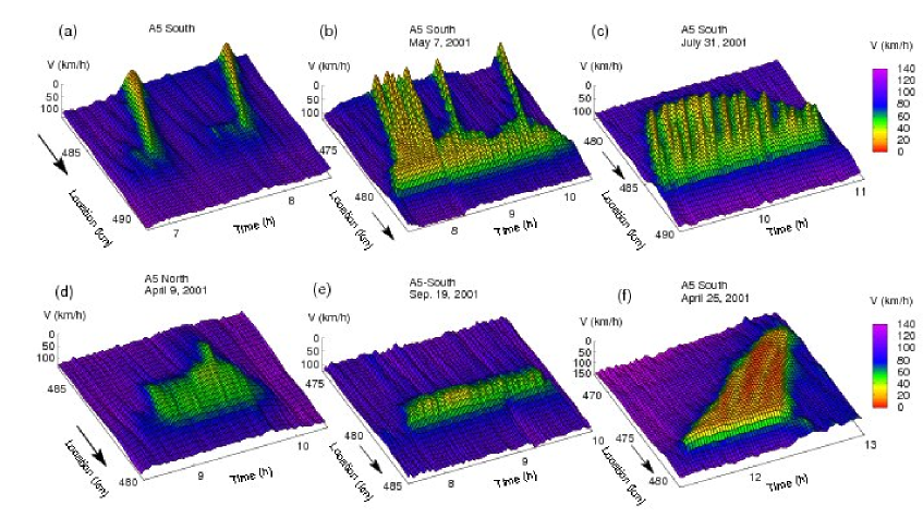
Figure 1: Examples of elementary patterns of congested traffic measured on the German freeway A5 close to Frankfurt. For better illustration of the traffic patterns, speeds are displayed upside down. The driving direction is indicated by arrows. Top row: (a) Moving clusters (MC), (b) stop-and-go waves (SGW), (c) oscillating congested traffic (OCT). Bottom row: (d) Widening synchronized pattern (WSP), (e) pinned localized cluster (PLC), and (f) homogeneous congested traffic (HCT). The spatiotemporal velocity fields have been reconstructed from one-minute data of double-loop detector cross sections using the “adaptive smoothing method” protectTreiber-smooth .

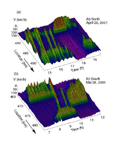
Figure 2: Two examples of complex traffic states measured on the German freeway A5 close to Frankfurt. Top: On the A5 North, an accident occurs at $x=487.5$ km at the time $t=17$:13 h, which causes a HCT pattern that turns into an OCT pattern as the upstream traffic flow goes down. The capacity drop related to the congestion pattern reduces the downstream flow and leads to a dissolution of the previous SGW pattern over there around $t=18$:00 h. Bottom: On the freeway A5 South, the stop-and-go waves induced by a bottleneck at $x=480$ km replace the OCT at the bottleneck near $x=470$ km. At time $t=9$:50 h, the waves induce an accident at $x=478.33$ km, which triggers a new OCT pattern further upstream. The related capacity drop, in turn, causes the previous OCT state at $x\approx 480$ km to dissolve.

It was proposed that the occurrence of elementary congested traffic states could be classified and predicted by a phase diagram Phase ; Opus . Furthermore, it was suggested that this phase diagram can be derived from the instability diagram of traffic flow and the outflow from congested traffic. This idea has been taken up in many other publications, also as a means of studying, visualizing, and classifying properties of traffic models Lee99 ; Lee-emp ; Barlovic-phasediag ; CA-phasediag . However, it has been claimed that the phase diagram approach would be insufficient Kerner-book . While some of the criticism is due to misunderstandings, as will be shown in Sec. 7.1, the classical phase diagrams lack, in fact, the possibility of “widening synchronized patterns” (WSP) proposed by Kerner and Klenov Kerner-Mic , see Fig. 1(d).

In this paper, we will start in Sec. 2 with a discussion of the somewhat controversial notion of “traffic phases” and the clarification that we use it to distinguish congestion patterns with a qualitatively different spatiotemporal appearance. In Sec. 3 we will show that existing models can produce all the empirically observed patterns of Fig. 1, when simulated in an open system with a bottleneck. We will then present a derivation and explanation of the idealized, schematic phase diagram of traffic states in Sec. 4. In contrast to previous publications, we will assume that the critical density $\rho_{\rm c2}$, at which traffic becomes linearly unstable, is greater than the density $\rho_{\rm max}$, where the maximum flow is reached (see Appendix A for details). As a consequence, we will find that “widening synchronized pattern” do exist within the phase diagram approach, even for models with a fundamental diagram. While this analysis is carried out for single, isolated bottlenecks, Sec. 5 will introduce how to generalize it to the case of multi-ramp setups. In Sec. 6, we will discuss other possible types of phase diagrams, depending on the stability properties of the considered model. Afterwards, in Sec. 7, we will present recent empirical data supporting our theoretical phase diagram. Sections 7.1 and 8 will finally try to overcome some misunderstandings regarding the phase diagram concept and summarize our findings.

2 On the Definition of Traffic Phases

Before we present the phase diagram of traffic states, it must be emphasized that some confusion arises from the different use of the term “(traffic) phase”. In thermodynamics, a “phase” corresponds to an equilibrium state in a region of the parameter space of thermodynamic variables (such as pressure and temperature), in which the appropriate free energy is analytic, i.e., all first and higher-order derivatives with respect to the thermodynamic variables exist. One speaks of a first-order phase transition, if a first derivative, or “order parameter”, is discontinuous, and of a “second-order” or “continuous” phase transition, if the first derivatives are continuous but a second derivative (the “susceptibility”) diverges. What consequences does this have for defining “traffic phases”?

Although traffic flow is a self-driven nonequilibrium system, it has been shown Arndt-nonlinThermo that much of the equilibrium concepts can be transferred to driven or self-driven non-equilibrium systems by appropriately redefining them. Furthermore, concepts of classical thermodynamics have been successfully applied to nonequilibrium physical and nonphysical systems, yielding quantitatively correct results. This includes, for example, the application of the fluctuation-dissipation theorem FDT (originally referring to equilibrium phenomena) to vehicular traffic FPE-EuroPhys08 .

In contrast to classical thermodynamics, nonequilibrium phase transitions are possible in one-dimensional systems Eva98 . However, according to the definition of phase transitions, one needs to make sure that details of the boundary conditions or finite-size effects do not play a role for the characteristic properties of the phase. Furthermore, one must define suitable order parameters or susceptibilities. While the first propositions have been already made a decade ago Lubeck-98 , there is no general agreement regarding the quantity that should be chosen for the order parameter. Candidates include the density, the fraction of vehicles in the congested state Lubeck-98 , the average velocity or flow, or the variance of density, velocity, or flow. Whenever one observes a discontinuous or hysteretic transition in a large enough system, there is no need to define an order parameter, as this already implies a first-order phase transition. For continuous, symmetry-braking phase transitions, the deviation from the more symmetric state (e.g. the amplitude of density variations as compared to the homogeneous state) seems to be an appropriate order parameter.

To summarize the above points, it appears that thermodynamic phases can, in fact, be defined for traffic flow. In connection with transitions between different traffic states at bottlenecks, we particularly mention the notion of boundary-induced phase transitions KrugLetter ; schuetz ; Popkov-boundaryPhase . Here, the boundary conditions have been mainly used as a means to control the average density in the open system under consideration.

In publications on traffic, a “phase” is often interpreted as “traffic pattern” or “traffic state with a typical spatio-temporal appearance”. Such states depend on the respective boundary conditions. In this way, models with several phases can produce a multitude of spatiotemporal patterns. It should become clear from these considerations that the various proposed “phase diagrams” do not relate to thermodynamic phases, but classify spatio-temporal states, as is common in systems theory. In these non-thermodynamic phase diagrams, the “phase space” is spanned by certain control parameters, e.g. by suitably parameterized boundary conditions, by inhomogeneities (bottleneck strengths), or by model parameters HDM . For example, the phase diagrams discussed in Refs. Phase ; Kerner-book and this paper contain the axes “main inflow” (i.e., an upstream boundary condition) and “on-ramp flow” (characterizing the bottleneck strength).

In any case, empirical observations of the traffic dynamics relate to the spatiotemporal traffic patterns, and not to the thermodynamic phases. Therefore, the quality of a traffic model should be assessed by asking whether it can produce all observed kinds of spatio-temporal traffic patterns, including the conditions for their appearance.

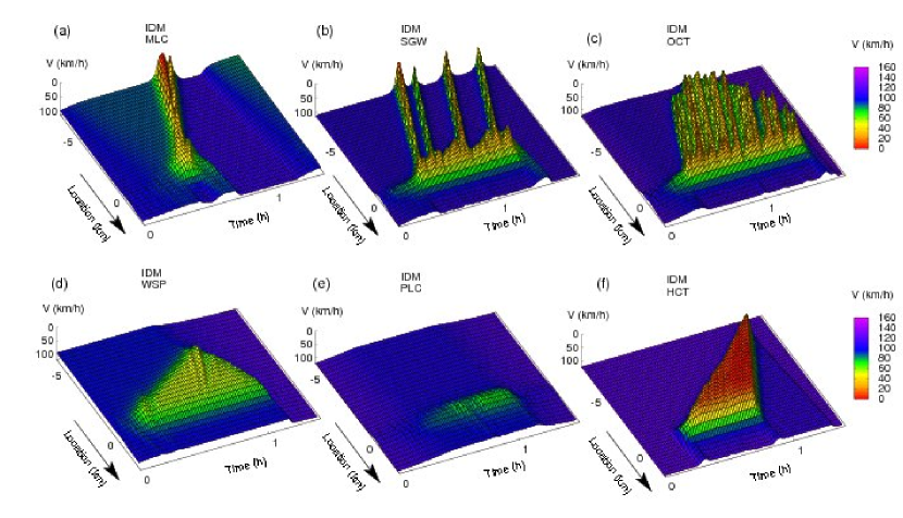
Figure 3: Simulation of traffic on a freeway with an on-ramp at location $x=0$ km using the intelligent driver model (IDM) Opus with parameters corresponding to an instability diagram as illustrated in Fig. 4(d). The macroscopic velocity field was extracted from the simulated trajectories by placing virtual detectors every 500 m and determining the velocity with the same method Treiber-smooth that has been used for the data. Depending on the respective traffic flows on the ramp and on the freeway, different kinds of congested traffic states emerge: a moving cluster (MC), a pinned localized cluster (PLC), (“triggered”) stop-and-go waves (SGW), oscillating congested traffic (OCT), or homogeneous congested traffic (HCT). During the first minutes of the simulation, the flows on the freeway and the on-ramp were increased from low values to their final values. Since the assumed flows fall into a metastable traffic regime, the actual breakdown was initiated by additional perturbations of the ramp flow.

3 Congested Traffic States

When simulating traffic flow with the “microscopic” intelligent driver model (IDM) Opus , the optimal velocity model (OVM) Bando-98 , the non-local, gas-kinetic-based traffic model (GKT) GKT , or the “macroscopic” Kerner-Konhäuser model KeKo93 (with the parameter set chosen by Lee et al. Lee ), we find free traffic flow and different kinds of congestion patterns, when the ramp flow $Q_{\rm on}$ and the upstream arrival flow $Q_{\rm up}$ on the freeway are varied. The diversity of traffic patterns is

1. due to the possibility of having either locally constraint or spatially extended congestion and

2. due to the possibility of having stable, unstable or free traffic flows.

Typical representatives of congested traffic patterns obtained by computer simulations with the intelligent driver model Opus are shown in Fig. 3. Notice that all empirical patterns displayed in Fig. 1 can be reproduced.

One can distinguish the different traffic states (i.e. congestion patterns) by analyzing the temporal and spatial dependence of the average velocity $V(x,t)$: If $V(x,t)$ stays above a certain threshold $V_{\rm crit}$, where $x$ is varied within a homogeneous freeway section upstream of a bottleneck, we call the traffic state free traffic (FT), otherwise congested traffic. If these speeds fall below $V_{\rm crit}$ only over a short freeway subsection, and the length of this section is approximately stable or stabilizes over time, we talk about localized clusters (LC), otherwise of spatially extended congestion states (see also footnote 1).

According to our simulations, there are two forms of localized clusters: Pinned localized clusters (PLC) stay at a fixed location over a longer period of time, while moving localized clusters (MLC) propagate upstream with the characteristic speed $c_{0}$. These states have to be contrasted with extended congested traffic: Stop-and-go waves (SGW) may be interpreted as a sequence of several moving localized clusters. Alternatively, they may be viewed as special case of oscillating congested traffic (OCT), but with free traffic flows of about $Q_{\rm out}\gtrsim 1800$ vehicles/h/lane between the upstream propagating jams. Generally, however, OCT is just characterized by oscillating speeds in the congested range, i.e. unstable traffic flows. If the speeds are congested over a spatially extended area, but not oscillating, we call this homogeneous congested traffic (HCT). It is typically related with low vehicle velocities.

In summary, besides free traffic, the above mentioned and some other traffic models predict five different, spatio-temporal patterns of congested traffic states at a simple on-ramp bottleneck: PLC, MLC, SGW, OCT, and HCT. Similar traffic states have been identified for flow-conserving bottlenecks in car-following models Helb-Opus ; Helb-micmac , and for on-ramps and other types of bottlenecks in macroscopic models Phase ; Lee .

In contrast to this past work, we have also simulated an additional traffic pattern [Fig. 3(d)]. This pattern has a similarity to the widening synchronized pattern (WSP) proposed by Kerner in the framework of his three-phase traffic theory BKernerKlenov-02 . In the following section, we show how this pattern may be understood in the framework of models with a fundamental diagram.

4 Derivation and Explanation of the Phase Diagram of Traffic States

It turns out that the possible traffic patterns in open systems with bottlenecks are mainly determined by the instability diagram (see Fig. 4), no matter if the model is macroscopic or microscopic. This seems to apply at least for traffic models with a fundamental diagram, which we will focus on in the following sections. Due to the close relationship with the instability diagram, the preconditions for the possible occurrence of the different traffic states can be illustrated by a phase diagram. Figures 5 and 6 show two examples. Each area of a phase diagram represents the combinations of upstream freeway flows $Q_{\rm up}$ and bottleneck strengths $\Delta Q$, for which a certain kind of traffic state can exist.

It is obvious that an on-ramp flow $Q_{\rm on}(t)$, for example, causes a bottleneck, as it consumes some of the capacity of the freeway. $Q_{\rm on}(t)$ represents the flow actually entering the freeway via the on-ramp, i.e. the flow leaving the on-ramp and not the flow entering the on-ramp. We assume that $Q_{\rm on}(t)$ is known through a suitable measurement. Having clarified this, we define the bottleneck strength due to an on-ramp by the entering ramp flow, divided by the number $I_{\rm fr}$ of freeway lanes:

$$\Delta Q(t)=\Delta Q_{\rm on}(t)=\frac{Q_{\rm on}(t)}{I_{\rm fr}}\,.$$ (1)

This is done so, because the average flow $\Delta Q$ added to each freeway lane by the on-ramp flow corresponds to the capacity that is not available anymore for the traffic flow $Q_{\rm up}$ coming from the upstream freeway section. As a consequence, congestion may form upstream of the ramp. In the following, we will have to determine the density inside the forming congestion pattern and where in the instability diagram it is located. It will turn out that, given certain values of $Q_{\rm up}$ and $\Delta Q$, the different regions of the phase diagram can be related with the respectively observed or simulated spatiotemporal patterns. We distinguish free traffic and different kinds of localized congested traffic as well as different kinds of extended congested traffic. When contrasting our classification of traffic states with Kerner’s one Kerner-book , we find the following comparison helpful:

1. According to our understanding, what we call “extended congested traffic” may be associated with Kerner’s “synchronized flow”. In particular, the area where Kerner’s phase diagrams predict a “general pattern” matches well with the area, where we expect OCT and HCT states.

2. “Moving clusters” may be associated with “wide moving jams” and/or “moving synchronized patterns” (MSP).

3. “Stop-and-go waves” appear to be related with multiple “wide moving jams” generated by the “pinch effect”.

4. “Pinned localized clusters” may related to Kerner’s “localized synchronized pattern” (LSP).

5. Kerner’s “widening synchronized pattern” (WSP) and “dissolving general pattern” (DGP) did not have a correspondence with results of our own computer simulations so far. These states are predicted to appear for high freeway flows and low bottleneck strengths. In the following subsections, we report that, quite unexpectedly, similar results are found for certain traffic models having a fundamental diagram.

The phase diagram can not only be determined numerically. It turns out that the borderlines between different areas (the so-called phase boundaries) can also be theoretically understood, based on the flows

$$Q_{{\rm c}k}=Q_{\rm e}(\rho_{{\rm c}k})$$ (2)

at the instability thresholds $\rho_{{\rm c}k}$ ($k=1,\ldots,4$), the maximum flow capacity $Q_{\rm max}$ under free flow conditions, and the dynamic flow capacity, i.e. the characteristic outflow ${Q}_{\rm out}$ from congested traffic Kerner-Rehb96 (see Fig. 4). $Q_{\rm e}(\rho)$ represents the equilibrium flow-density relationship, which is also called the “fundamental diagram”.

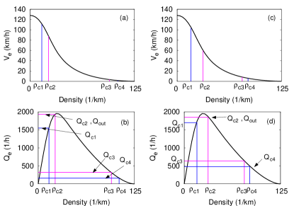
Figure 4: Illustration of stable, linearly unstable, and metastable density regimes within velocity-density diagrams $V_{\rm e}(\rho)$ (top) and the flow-density diagrams $Q_{\rm e}(\rho)$ (bottom). Traffic is stable for $\rho<\rho_{c1}$ and $\rho>\rho_{c4}$ and linearly unstable for $\rho_{c2}<\rho<\rho_{c3}$. These two regimes are separated by a low-density and a high-density region of metastable traffic given by the intervals $\rho_{c1}<\rho<\rho_{c2}$ and $\rho_{c3}<\rho<\rho_{c4}$, respectively. In the metastable regimes, perturbations in the traffic flow grow, if their size is larger than a certain critical amplitude HelbMoussaid-EPJB-08 , otherwise they fade away. The critical amplitude is largest towards the boundaries $\rho_{\rm c1}$ and $\rho_{\rm c4}$ of unconditionally stable traffic flow, while it goes to zero towards the boundaries $\rho_{\rm c2}$ and $\rho_{\rm c3}$ of linearly unstable traffic. Note that the metastable and unstable regimes may vanish for certain traffic models or parameter specifications. The possible types of congested traffic patterns depend on the existence of the different stability regimes and on the relative position of their boundaries with respect to the density $\rho_{\rm max}$ at capacity $Q_{\rm max}$ (maximum flow). The left figures show the situation for $\rho_{c2}<\rho_{\rm max}$, the right figures the situation for $\rho_{c2}>\rho_{\rm max}$.

The exact shape and location of the separation lines between different kinds of traffic states depend on the traffic model and its parameter values. Furthermore, the characteristic outflow ${Q}_{\rm out}$ typically depends on the type and strength of the bottleneck. For the sake of simplicity of our discussion, however, we will assume constant outflows $Q_{\rm out}$ in the following.

The meaning of the different critical density thresholds $\rho_{{\rm c}k}$ and flow thresholds $Q_{{\rm c}k}=Q_{\rm e}(\rho_{{\rm c}k})$, respectively, is described in the caption of Fig. 4. Note that the density $\rho_{{\rm c}2}$ may be smaller or larger than the density $\rho_{\rm max}$ at capacity, where the maximum flow $Q_{\rm max}$ is reached. Previous computer simulations and phase diagrams mostly assumed parameters where traffic at capacity is linearly unstable ($\rho_{{\rm c}2}<\rho_{\rm max}<\rho_{{\rm c}3}$), which is depicted in Figs. 4(a) and (b). However, in some traffic models such as the IDM Opus , the stability thresholds can be controlled in a flexible way by varying their model parameters (see Appendix B). In the following, we will focus on the case where traffic at capacity is metastable ($\rho_{\rm c2}>\rho_{\rm max}>\rho_{\rm c1}$), cf. Fig. 4(c) and (d). As will be shown in the next subsection, this appears to offer an alternative explanation of the “widening synchronized pattern” (WSP) introduced in Ref. BKernerKlenov-02 , see Fig. 3(d). Simpler cases will be addressed in Sec. 6 below.

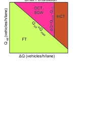
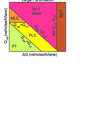
Figure 5: Schematic (idealized) phase diagrams for the expected traffic patterns as a function of the upstream freeway flow $Q_{\rm up}$ and the ramp flow $\Delta Q$, as studied in Refs. Phase ; Opus . The left figure is for negligible, the right figure for large perturbations. The situation for medium-sized perturbations can lie anywhere between these two extremes. For example, in the area marked as PLC, one may find free traffic or pinned localized clusters, or in some of the area attributed to HCT, one may find SGW or OCT states. The assumed instability diagram underlying the above schematic phase diagrams is depicted in Figs. 4(a) and (b). With $\rho_{\rm c1}<\rho_{\rm c2}<\rho_{\rm max}<\rho_{\rm c3}<\rho_{\rm c4}<\rho_{\text{jam}}$, it assumes no degeneration of the critical densities $\rho_{{\rm c}k}$ and a stable flow at high densities. Note that, for illustrative reasons, we have set aside the exact correspondence of the flow values $Q_{{\rm c}k}$.

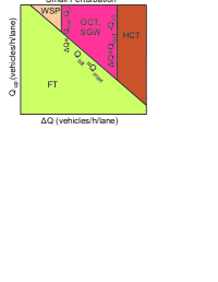
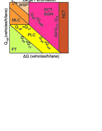
Figure 6: Schematic phase diagram as in Fig. 5, but for the instability diagram represented by Figs. 4(c) and (d). In contrast to Fig. 5, traffic flow at capacity is metastable ($\rho_{c1}<\rho_{\rm max}<\rho_{c2}$), which leads to a greater variety of traffic states in the upper left corner of the phase diagram. In particularly, we find “widening synchronized patterns” (WSP). “OCT, SGW” means that one expects to find oscillating congested traffic or stop-and-go waves, but not necessarily both. Together with “widening moving clusters” (WMC, see footnote 1) they form the area of extended oscillatory congestion. However, the WMC and MLC phases may also be summarized by one area representing “moving clusters” (MC).

4.1 Transition to Congested Traffic for Small Bottlenecks

In the following, we restrict our considerations to situations with one bottleneck only, namely a single on-ramp. Combinations of off- and on-ramps are not covered by this section. They will be treated later on (see Sec. 5).

For matters of illustration, we assume a typical rush hour scenario, in which the total traffic volume

$$Q_{\rm tot}(t)=Q_{\rm up}(t)+\Delta Q(t)\,,$$ (3)

i.e. the sum of the flow $Q_{\rm up}(t)$ sufficiently upstream of the ramp bottleneck and the on-ramp flow $\Delta Q(t)$ per freeway lane, is increasing with time $t$. As long as traffic flows freely, the flow downstream of the bottleneck corresponds to the total flow $Q_{\rm tot}(t)$, while the upstream flow is $Q_{\rm up}(t)$.

When the total flow $Q_{\rm tot}(t)$ exceeds the critical density $\rho_{\rm c1}$, it enters the metastable density regime. That is, large enough perturbations may potentially grow and cause a breakdown of the traffic flow. However, often the perturbations remain comparatively small, and the total traffic volume rises so quickly that it eventually exceeds the maximum freeway capacity

$$Q_{\rm tot}=Q_{\rm up}+\Delta Q>Q_{\rm max}=\max_{\rho}Q_{\rm e}(\rho)=Q_{\rm e}(\rho_{\rm max})\,.$$ (4)

This is reflected in the left phase diagram in Fig. 6 by the diagonal line separating the states “FT” and “WSP”. (Note that $\rho_{\rm max}$ represents the density, for which the maximum free traffic flow occurs, not the jam density $\rho_{\rm jam}$.)

When the total traffic volume $Q_{\rm tot}$ exceeds the maximum capacity $Q_{\rm max}$, a platoon of vehicles will form upstream of the bottleneck. Since, in this section, we assume metastable traffic at maximum capacity $Q_{\rm max}$ (see Fig. 7 in Ref. HelbTilch-EPJB-08 ), this will not instantaneously lead to a traffic breakdown with an associated capacity drop. Thus, the flow downstream of the bottleneck remains limited to $Q_{\rm max}$ (at least temporarily). As the on-ramp flow takes away an amount $\Delta Q$ of the maximum capacity $Q_{\rm max}$, the (maximum) flow upstream of the bottleneck is given by

$$Q_{\rm bot}=Q_{\rm max}-\Delta Q\,.$$ (5)

When the actual upstream flow $Q_{\rm up}$ exceeds this value, a mild form of congestion will result upstream of the ramp. The density of the forming vehicle platoon is predicted to be

$$\rho_{\rm bot}=\rho_{\rm cg}(Q_{\rm bot})=\rho_{\rm cg}\big{(}Q_{\rm max}-\Delta Q\big{)}>\rho_{\rm max}\,,$$ (6)

where $\rho_{\rm cg}(Q)$ is the density corresponding to a stationary and homogeneous congested flow of value $Q$ (i.e. it is the inverse function of the “congested branch” of the fundamental diagram).

According to the equation for the propagation speed of shockwaves (see Ref. Whitham74 ), the upstream front of the forming vehicle platoon is expected to propagate upstream at the speed

$$C_{1}(t)=\frac{Q_{\rm up}-Q_{\rm bot}}{\rho_{\rm fr}(Q_{\rm up})-\rho_{\rm cg}(Q_{\rm bot})}\,,$$ (7)

where $\rho_{\rm fr}(Q)$ is the density of stationary and homogeneous traffic at a given flow $Q$ (i.e. the inverse function of the “free branch” of the fundamental diagram.)

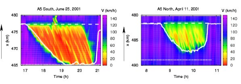
Figure 7: Examples of congestion patterns on the German freeway A5 close to Frankfurt, for which data have been provided to the authors between kilometers 465 and 492. The figures analyze the propagation of the upstream front of a region of congested traffic (white solid line) according to Eq. (12), for empirical HCT (left) and OCT (right). In both plots, the driving direction is upwards (as indicated by the arrows). The upstream flow $Q_{\text{up}}$ was determined from a detector cross section whose location is indicated by a dotted white line, while the bottleneck flow was determined from detectors of a nearby cross section (dashed white line). When determining the flows, the time delay caused by the finite propagation velocities $dQ_{\text{e}}(\rho)/d\rho$ from the detectors to the upstream front was taken care of. The congestion patterns were chosen such that there were no ramps at or between the two detector cross sections. Otherwise, the determination of $Q_{\text{up}}$ and $Q_{\text{cong}}$ would have been more complicated. The free and congested densities were calculated with a simple, triangular fundamental diagram. Therefore, $\rho_{\text{fr}}(Q)=Q/V_{0}$ and $\rho_{\text{cg}}(Q)=\rho_{\text{jam}}(1-QT)$, where the following parameters were chosen: $V_{0}=120\,\mathrm{km/h}$, $\rho_{\text{jam}}=100\,\mathrm{veh/km/lane}$, and $T=2\,\mathrm{s}$.

Note that this high-flow situation can persist for a significant time period only, if the flow $Q_{\rm bot}$ in the platoon is stable or metastable. This is the case if one of the following applies:

• The traffic flow is unconditionally stable for all densities such as in the Lighthill-Whitham model Lighthill-W . This will be discussed in Sec. 6 below.

• Traffic flow at capacity is metastable and the bottleneck is sufficiently weak. This gives rise to the widening synchronized pattern (WSP), as will be discussed in the rest of this subsection.

By WSP, we mean a semi-congested extending traffic state without large-scale oscillations or significant velocity drops below, say, 30-40 km/h Kerner-book . Putting aside stochastic accelerations or heterogeneous driver-vehicle populations, this corresponds to (meta-)stable vehicle platoons at densities greater than, but close to the density $\rho_{\rm max}$ at capacity. This can occur when $\rho_{\rm bot}$ lies in the metastable density range, i.e. $\rho_{\rm max}<\rho_{\rm bot}<\rho_{\rm c2}$, corresponding to $Q_{\rm max}>Q_{\rm bot}=Q_{\rm max}-\Delta Q>Q_{\rm c2}$ or

$$\Delta Q<Q_{\rm max}-Q_{\rm c2}.$$ (8)

In Fig. 6, this condition belongs to the area left of the vertical line separating the WSP and OCT states. If the bottleneck strength $\Delta Q$ becomes greater than $Q_{\rm max}-Q_{\rm c2}$, or if $\rho_{\rm cg}(Q_{\rm bot})$ lies in the metastable regime and perturbations in the traffic flow are large enough, traffic flow becomes unstable and breaks down. After the related capacity drop by the amount

$$\Delta Q_{\rm drop}=Q_{\rm max}-Q_{\rm out}\,,$$ (9)

the new, “dynamic” capacity will be given by the outflow $Q_{\rm out}$ from congested traffic Opus . Obviously, the capacity drop causes the formation of more serious congestion. This is illustrated in the right phase diagram of Fig. 6 by the offset between the diagonal lines separating free traffic from WSP and the other extended congested states (OCT, SGW, and HCT). In the following, we will focus on the traffic states after the breakdown of freeway capacity from $Q_{\rm max}$ to $Q_{\rm out}$ has taken place.

4.2 Conditions for Different Kinds of Congested Traffic after the Breakdown of Traffic Flow

For the sake of simplicity, we will assume the case

$$Q_{\rm c4}<Q_{\rm c3}<Q_{\rm c1}\leq Q_{\rm out}\leq Q_{\rm c2}<Q_{\rm max}\,,$$ (10)

which seems to be appropriate for real traffic (particularly in Germany). However, depending on the choice of model parameters, other cases are possible. The conclusions may be different, then, but the line of argumentation is the same. In the following, we will again assume $\rho_{\rm c2}\geq\rho_{\rm max}$, so that the maximum flow $Q_{\rm max}$ is metastable. Therefore, it can persist for some time, until the maximum flow state is destabilized by perturbations or too high traffic volumes $Q_{\rm tot}(t)$, which eventually cause a breakdown of the traffic flow. (For $\rho_{\rm c2}<\rho_{\rm max}$, the capacity drop happens automatically, whenever $Q_{\rm tot}(t)>Q_{\rm max}$.)

After the breakdown of traffic flow, the traffic situation downstream is given by the outflow $Q_{\rm out}$ from (seriously) congested traffic. As the actually entering ramp flow requires the capacity $\Delta Q$ per lane, the flow upstream of the bottleneck is limited to

$$Q_{\rm cong}=Q_{\rm out}-\Delta Q\,.$$ (11)

In analogy to Eq. (7), the upstream front of this congested flow is expected to propagate with the velocity

$$C_{2}(t)=\frac{Q_{\rm up}-Q_{\rm cong}}{\rho_{\rm fr}(Q_{\rm up})-\rho_{\rm cg}(Q_{\rm cong})}\,,$$ (12)

as the upstream freeway flow $Q_{\rm up}$ is assumed to be free. The downstream end of the congested flow $Q_{\rm cong}$ remains located at the bottleneck helbing-sectionbased03 .

Figure 7 shows that the propagation of the upstream front according to Eq. (12) agrees remarkably well with empirical observations, not only for homogeneous congested flow but also for the OCT pattern. Since the location of the congestion front is given by integration of Eq. (12) over time, oscillations of the input quantities of this equation are automatically averaged out.

The resulting congestion pattern depends on the stability properties of the vehicle density

$$\rho_{\rm cong}=\rho_{\rm cg}(Q_{\rm cong})=\rho_{\rm cg}\big{(}Q_{\rm out}-\Delta Q\big{)}$$ (13)

in the congested area, where the outflow $Q_{\rm out}$ from seriously congested traffic represents the effective freeway capacity under congested conditions and $\Delta Q$ the capacity taken away by the bottleneck. In view of this stability dependence, let us now discuss the meaning of the critical densities $\rho_{{\rm c}k}$ or associated flows $Q_{{\rm c}k}=Q_{\rm e}(\rho_{{\rm c}k})$, respectively, for the phase diagram.

If $\rho_{\rm c2}<\rho_{\rm cong}<\rho_{\rm c3}$, we expect unstable, oscillatory traffic flow (OCT or SGW). For $\rho_{\rm c3}\leq\rho_{\rm cong}<\rho_{\rm c4}$, the congested flow is metastable, i.e. it depends on the perturbation amplitude: One may either have oscillatory patterns (for large enough perturbations) or homogeneous ones (for small perturbations). Moreover, for $\rho_{\rm cong}\geq\rho_{\rm c4}$ (given that the critical density $\rho_{\rm c4}$ is smaller than $\rho_{\rm jam}$), we expect homogeneous, i.e. non-oscillatory traffic flows.

Expressing this in terms of flows rather than densities, one would expect the following: Oscillatory congestion patterns (OCT or SGW) should be possible for $Q_{\rm c2}>Q_{\rm cong}=Q_{\rm out}-\Delta Q>Q_{\rm c4}$, i.e. in the range

$$Q_{\rm out}-Q_{\rm c2}<\Delta Q<Q_{\rm out}-Q_{\rm c4}\,,$$ (14)

where we have considered $Q_{\rm c2}\geq Q_{\rm out}$.

The assumption that the densities between $\rho_{\rm out}$ with $Q_{\rm e}(\rho_{\rm out})=Q_{\rm out}$ and $Q_{\rm max}$ are metastable, as we assume here, has interesting implications: A linear instability would cause a single moving cluster to trigger further local clusters and, thereby, so-called “triggered stop-and-go waves” (TSG or SGW) Phase . A metastability, in contrast, can suppress the triggering of additional moving clusters, which allows the persistence of a single moving cluster, if the bottleneck strength $\Delta Q$ is small. As, for $Q_{\rm tot}>Q_{\rm out}$, the related flow conditions fall into the area of extended congested traffic, the spatial extension of such a cluster will grow. Therefore, one may use the term “widening moving cluster” (WMC).

Furthermore, according to our computer simulations, the capacity downstream of a widening moving cluster may eventually revert from $Q_{\rm out}$ to $Q_{\rm max}$. This happens in the area, where “widening synchronized patterns” (WSP) can appear. Therefore, rather than by Eq. (14), the bottleneck strengths characterizing OCT or SGW states are actually given by

$$Q_{\rm max}-Q_{\rm c2}<\Delta Q<Q_{\rm out}-Q_{\rm c4}\,,$$ (15)

where the lower boundary corresponds to the boundary of the WSP state, see Eq. (8). We point out that a capacity reversion despite congestion is a special feature of traffic models with $\rho_{\rm c2}>\rho_{\rm max}$.

Homogeneous congested traffic (the definition of which does not cover the homogeneous WSP state) is expected to be possible for $Q_{\rm cong}=Q_{\rm out}-\Delta Q<Q_{\rm c3}$, i.e. (meta-) stable flows at high densities. This corresponds to

$$\Delta Q>Q_{\rm out}-Q_{\rm c3}\,.$$ (16)

The occurrence of extended congested traffic like HCT and OCT requires an additional condition: The total flow must exceed the freeway capacity $Q_{\rm out}$ during serious congestion, i.e. we must have

$$Q_{\rm tot}=Q_{\rm up}+\Delta Q>Q_{\rm out}\,.$$ (17)

Localized congestion patterns, in contrast, require $Q_{\rm tot}\leq Q_{\rm out}$ and can be triggered for $Q_{\rm tot}>Q_{\rm c1}$, which implies

$$Q_{\rm c1}<Q_{\rm tot}=Q_{\rm up}+\Delta Q\leq Q_{\rm out}\,.$$ (18)

We can distinguish at least two cases: On the one hand, if

$$Q_{\rm c1}<Q_{\rm up}<Q_{\rm max}\,,$$ (19)

the flow upstream of the congested area is metastable, which allows jams (and large enough perturbations) to propagate upstream. In this case, we speak of moving localized clusters (MLC). Their propagation speed $c_{0}=-15\pm 5$ km/h is given by the slope of the jam line Kerner-98e .

On the other hand, if

$$Q_{\rm up}\leq Q_{\rm c1}$$ (20)

or $\rho_{\rm fr}(Q_{\rm up})<\rho_{\rm c1}$, traffic flow upstream of the bottleneck is stable. Under such conditions, perturbations and, in particular, localized congestion patterns cannot propagate upstream, and they stay at the location of the bottleneck. In this case, one speaks of pinned localized clusters (PLC).

We underline that the actual outflow $\tilde{Q}_{\rm out}$ from localized clusters corresponds, of course, to their inflow $Q_{\rm up}+\Delta Q$ (otherwise they would grow or shrink in space). Therefore, the actual outflow $\tilde{Q}_{\rm out}$ of localized congestion patterns can be smaller than $Q_{\rm out}$, i.e. smaller than the outflow of serious congestion.

5 Combinations of On- and Off-Ramps

We see that the instability diagram implies a large variety of congestion patterns already in the simple simulation scenario of a homogeneous freeway with a single ramp. The possible congestion patterns are even richer in cases of complex freeway setups. All combinations of the previously discussed, “elementary” traffic patterns are possible. Furthermore, we expect particular patterns due to interactions among patterns through spillover effects. For illustration, let us focus here on the combination of an on-ramp with an off-ramp further upstream. This freeway design is illustrated in Fig. 8 and often built to reduce the magnitude of traffic breakdowns, since it is favorable when vehicles leave the freeway before new ones enter. Nevertheless, the on-ramp and the off-ramp bottleneck can get coupled, namely when congestion upstream of the on-ramp reaches the location of the off-ramp.

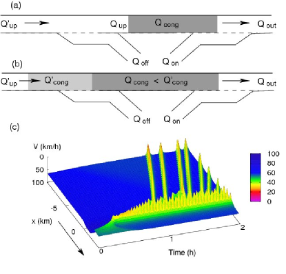
Figure 8: Combination of an on-ramp bottleneck with an upstream off-ramp. (a) When the flow $Q_{\rm up}=Q^{\prime}_{\rm up}-\Delta Q_{\rm off}$ upstream of the on-ramp exceeds $Q_{\rm cong}$, which is defined as the outflow $Q_{\rm out}$ from congested traffic minus the on-ramp flow $\Delta Q_{\rm on}=Q_{\rm on}/I_{\rm fr}$, congested traffic upstream of the on-ramp (dark grey area) is expected to grow. (b) As soon as the congested area extends up to the location of the off-ramp, the off-ramp bottleneck is activated. Its effective outflow $Q^{\prime}_{\rm out}$ is given by the congested flow $Q_{\rm cong}$ upstream of the on-ramp, while congested flow $Q^{\prime}_{\rm cong}$ upstream of the off-ramp is higher by the amount $\Delta Q_{\rm off}=Q_{\rm off}/I_{\rm fr}$ of the off-ramp flow. (c) Spatiotemporal velocity field resulting from a computer simulation with the gas-kinetic-based traffic model (GKT) GKT , which allows to treat ramps easily. The arrow indicates the driving direction. One can clearly see pronounced stop-and-go waves emanating from an area of oscillating congested traffic.

What would a bottleneck analysis analogous to the one in Sec. 4 predict for this setup? In order to discuss this, let us again denote the outflow capacity downstream of the on-ramp by $Q_{\rm out}$, its bottleneck strength equivalent to the on-ramp flow $Q_{\rm rmp}=Q_{\rm on}$ by $\Delta Q_{\rm on}=Q_{\rm rmp}/I_{\rm fr}\geq 0$, the upstream flow by $Q_{\rm up}$, and the average congested flow resulting immediately upstream of the on-ramp by $Q_{\rm cong}$. In contrast, we will denote the same quantities relating to the area of the off-ramp by primes (^′), but we will introduce the abbreviation $-\Delta Q_{\rm off}=Q^{\prime}_{\rm rmp}/I_{\rm fr}\leq 0$ for the effect of the off-ramp flow $Q^{\prime}_{\rm rmp}\leq 0$.

According to Fig. 8, we observe the following dynamics: First, traffic breaks down at the strongest bottleneck, which is the on-ramp. If $Q_{\rm up}>Q_{\rm out}-\Delta Q_{\rm on}$, congested flow of size $Q_{\rm cong}=Q_{\rm out}-\Delta Q_{\rm on}$ expands, and eventually reaches the location of the off-ramp, see Fig. 8(a). Afterwards, the freeway capacity downstream of the off-ramp suddenly drops from $Q^{\prime}_{\rm out}=Q_{\rm out}$ to the congested flow

$$Q^{\prime}_{\rm out}=Q_{\rm cong}=Q_{\rm out}-\Delta Q_{\rm on}$$ (21)

due to a spillover effect. This abrupt change in the bottleneck capacity restricts the capacity for the flow upstream of the off-ramp to

$$Q^{\prime}_{\rm cong}=Q_{\rm cong}+\Delta Q_{\rm off}\geq Q_{\rm cong}\,.$$ (22)

This higher flow capacity implies either free flow or milder congestion upstream of the off-ramp. If $Q^{\prime}_{\rm cong}$ is smaller than the previous outflow capacity $Q_{\rm out}$, we have a bottleneck along the off-ramp, and its effective strength $\Delta Q$ is given by the difference of these values:

$$\Delta Q=Q_{\rm out}-(Q_{\rm cong}+\Delta Q_{\rm off})=\Delta Q_{\rm on}-\Delta Q_{\rm off}\,.$$ (23)

That is, the bottleneck strength is defined as the amount of outflow from congested traffic which cannot be served by the off-ramp and the downstream freeway flow. For $Q_{\rm cong}+\Delta Q_{\rm off}\geq Q_{\rm out}$, no bottleneck occurs, which corresponds to a bottleneck strength $\Delta Q=0$. This finally results in the expression

$$\Delta Q=\max(\Delta Q_{\rm on}-\Delta Q_{\rm off},0)\leq\Delta Q_{\rm on}$$ (24)

helbing-sectionbased03 . Whenever $\Delta Q_{\rm off}>\Delta Q_{\rm on}$, there is no effective bottleneck upstream of the off-ramp, i.e. the off-ramp bottleneck is de-activated. For $\Delta Q=\Delta Q_{\rm on}-\Delta Q_{\rm off}>0$, however, the resulting congested flow upstream of the off-ramp becomes

$$Q^{\prime}_{\rm cong}=Q^{\prime}_{\rm out}+\Delta Q_{\rm off}=Q_{\rm out}-\Delta Q_{\rm on}+\Delta Q_{\rm off}=Q_{\rm out}-\Delta Q\,.$$ (25)

In conclusion, if congested traffic upstream of an on-ramp reaches an upstream off-ramp, the off-ramp becomes a bottleneck of strength $\Delta Q$, which is given by the difference between the on-ramp and the off-ramp flows (or zero, if this difference would be negative).

Since $\Delta Q\leq\Delta Q_{\rm on}$ according to Eq. (24) and $Q^{\prime}_{\rm cong}\geq Q_{\rm cong}$ according to Eq. (22), the congestion upstream of the off-ramp tends to be “milder” than the congestion upstream of the on-ramp. The resulting traffic pattern is often characterized by homeogeneous or oscillating congested traffic between the off-ramp and the on-ramp, and by stop-and-go waves upstream of the off-ramp, i.e. it has typically the appearance of a “pinch effect” Kerner-Rehb96-2 (see Fig. 8c). For this reason, Kerner also calls the “pinch effect” a “general pattern” Kerner-book .

6 Other Phase Diagrams and Universality Classes of Models

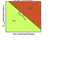
Figure 9: Schematic phase diagram for traffic flow without an extended linearly unstable density regime ($\rho_{c2}=\rho_{c3}$), when the traffic flow at capacity (at the density $\rho_{\rm max}$ corresponding to the maximum flow) is assumed to be metastable ($\rho_{c1}<\rho_{\rm max}<\rho_{c4}$).

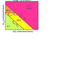
Figure 10: Schematic phase diagram for the case of an incomplete restabilisation at high densities, $\rho_{c3}<\rho_{c4}=\rho_{\text{jam}}$, when traffic at capacity is assumed to be linearly unstable ($\rho_{c1}<\rho_{c2}<\rho_{\rm max}$).

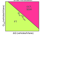
Figure 11: Schematic phase diagram for traffic flow exhibiting both, metastable and linearly unstable density regimes, with unstable flow at capacity ($\rho_{c1}<\rho_{c2}<\rho_{\rm max}$), but no restabilisation for very high densities ($\rho_{c3}=\rho_{c4}=\rho_{\text{jam}}$).

The phase diagram approach can also be used for a classification of traffic models. By today, there are hundreds of traffic models, and many models have a similar goodness of fit, when parameters are calibrated to empirical data HelbTilch-98ab ; Brockfeld-benchmark03 ; Brockfeld-benchmark04 ; Ossen-benchmark05 ; Ossen-interDriver06 ; Kesting-Calibration-TRR08 . It is, therefore, difficult, if not impossible, to determine “the best” traffic model. However, one can classify models according to topologically equivalent phase diagrams. Usually, there would be several models in the same universality class, producing qualitatively the same set of traffic patterns under roughly similar conditions. Among the models belonging to the same universality class, one could basically select any model. According to the above, the differences in the goodness of fit are usually not dramatic. Models with many model parameters may even suffer from insignificant parameters or parameters, which are hard to calibrate, at the cost of predictive power. Therefore, it is most reasonable to choose the simplest representative of a universality class which, however, should fulfil minimum requirements regarding theoretical consistency.

Before we enter the comparison with empirical data, let us discuss a number of phase diagrams expected for certain kinds of traffic models. Particular specifications of the optimal velocity model, for example, are linearly unstable for one density $\rho_{\rm c2}=\rho_{\rm c3}$ only, but show unstable behavior in an extended density regime for sufficiently large perturbations (i.e. extended metastable regimes) HelbMoussaid-EPJB-08 . The schematic phase diagram expected in this case is shown in Fig. 9. Some other traffic models have linearly unstable and metastable regimes, but do not show a restabilisation at very high densities, i.e. $\rho_{\rm c4}=\rho_{\text{jam}}$ (see Fig. 10), and sometimes one even has $\rho_{\rm c3}=\rho_{\text{jam}}$ siebel2006 ; KKW-CA (see Fig. 11). In the latter case, homogeneous congested traffic does not exist. In models such as the IDM, the restabilisation depends on the chosen parameter values Treiber-ThreePhasesTRB , see also Appendix B.

In most of the currently studied traffic models, one has either both, linearly unstable and metastable density ranges, or unconditionally stable traffic. In principle, however, models with linearly unstable but no metastable regimes are conceivable. For example, they may be established by taking a conventional model and introducing a dependence on the square of the velocity gradient (in macroscopic models) or the velocity difference (in microscopic models).

A linearly unstable model without metastable ranges would correspond to $\rho_{\rm c2}=\rho_{\rm c1}$ and $\rho_{\rm c4}=\rho_{\rm c3}$. For such models, we do not expect any multi-stability (see Fig. 12), and localized congested traffic would only be possible under special conditions Lee-emp ; Martin-empStates (e.g. on freeway sections between off- and on-ramps). If, in addition, there is no restabilisation (i.e. $\rho_{\rm c3}=\rho_{\text{jam}}$), only free traffic and oscillating congested traffic should exist. This seems to reflect the situation for the classical Nagel-Schreckenberg model Nagel-S , although the situation is somewhat unclear, since this model is stochastic and an exact distinction between free and congested states is difficult in this model.

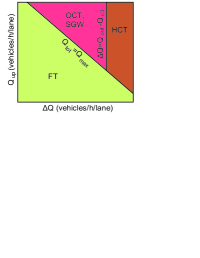
Figure 12: Schematic phase diagram, if there are only stable and linearly unstable, but no metastable density regimes ($\rho_{c1}=\rho_{c2}$, $\rho_{c3}=\rho_{c4}$). Furthermore, traffic at capacity is assumed to be unstable ($\rho_{c1}<\rho_{\rm max}<\rho_{c4}$)

Finally, we would like to discuss the fluid-dynamic model by Lighthill and Whitham Lighthill-W , which does not display any instabilities  Helb-Opus and, consequently, has only homogeneous patterns, namely free traffic for $Q_{\rm tot}\leq Q_{\rm max}$ and (homogeneous) extended congested traffic for $Q_{\rm tot}>Q_{\rm max}$ (which corresponds to a vehicle platoon behind the bottleneck). This is illustrated in Fig. 13. The two phases can also be distinguished locally, if temporal correlations are considered: While perturbations in free traffic travel in forward direction, in the congested regime they travel backward.

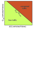
Figure 13: Schematic phase diagram, if traffic is unconditionally stable ($\rho_{c1}=\rho_{c2}=\rho_{c3}=\rho_{c4}$). The most prominent example is the Lighthill-Whitham model Lighthill-W , but many other models (including the gas-kinetic-based traffic model (GKT) GKT and the IDM) can be parameterized to reproduce this case.

We underline again that, by changing model parameters (corresponding to different driving styles), the resulting instability and phase diagrams of many traffic models change as well. For example, the IDM can be parameterized to generate most of the stability diagrams discussed in this contribution. Since different parameter values correspond to different driving styles or prevailing velocities, this may explain differences between empirical observations in different countries. For example, oscillating congested traffic seems to occur less frequent in the United States CasBer-99 ; Zielke-intlComparison .

Finally, note that somewhat different phase diagrams result for models that are characterized by a complex vehicle dynamics and no existence of a fundamental diagram KKW-CA ; Kerner-PhysA-04 . Nevertheless, similarities can be discovered (see Sec. 4).

7 Empirical Phase Diagram

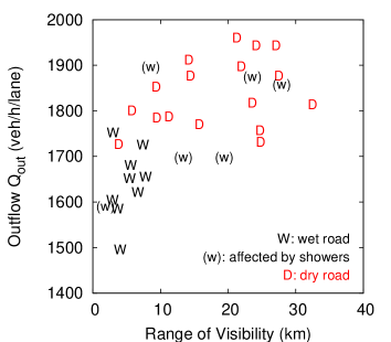
Figure 14: The outflows $Q_{\rm out}$ of congestion patterns correlate significantly with the weather-dependent range of visibility (meteorological optical range $3/\sigma$). This was determined by measuring the extinction coefficient $\sigma$, using multiple laser reflections. “W” denotes traffic breakdowns when the road surface was wet, while “D” stands for a dry road surface. Note that there are three cases of congestion marked with a lower-case “w”, which were related with a short and light shower only, so that the outflow values stayed comparatively high. For details see Ref. Schoenhof-Diss .

The remaining challenge in this paper is to find the universality class that fits the stylized facts of traffic dynamics well. Here, we will primarily demand that it fits the empirical phase diagram, i.e. reproduces all elementary congestion patterns observed, and not more. We have evaluated empirical data from the German freeway A5 close to Frankfurt. Due to the weather-dependence of the outflows $Q_{\rm out}$ (see Fig. 14), it is important to scale all flows by the respective measurements of $Q_{\rm out}$. This naturally collapses the area of localized congested traffic states to a line. As Fig. 15 shows, the phase diagram after scaling the flows is very well compatible with the theoretical phase diagrams of Figs. 5 and 6. Since the determination of the empirical phase diagram did not focus on the detection of “widening synchronized patterns”, it does not allow us to clearly distinguish between the two phase diagrams, i.e. to decide whether $\rho_{\rm c2}>\rho_{\rm max}$ or $\rho_{\rm c2}<\rho_{\rm max}$. However, the empirical WSP displayed in Fig. 1 suggests that Fig. 6 corresponding to $\rho_{\rm c2}>\rho_{\rm max}$ would be the right choice. Another piece of evidence for this is the metastability of vehicle platoons forming behind overtaking trucks (see Ref. HelbTilch-EPJB-08 ).

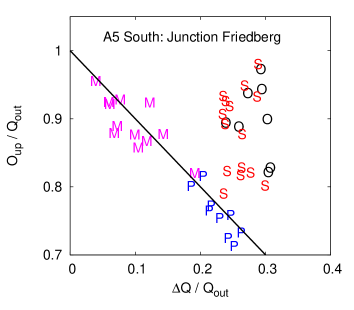
Figure 15: Empirical phase diagram, where the flows have been scaled by the respective outflows $Q_{\rm out}$ (after Martin-empStates ). The data represent the congested traffic states observed on the German freeway A5 at Junction Friedberg in direction South (M = moving localized cluster, S = stop-and-go waves, O = oscillating congested traffic, P = pinned localized cluster). It can be clearly seen that the non-extended traffic states are scattered around the line $Q_{\rm tot}/Q_{\rm out}=(Q_{\rm up}+\Delta Q)/Q_{\rm out}=1$, as expected, while the extended traffic states are above this line. Moreover, pinned localized clusters, moving localized clusters, and stop-and-go waves/oscillating congested traffic are well separated from each other. Homogeneous congested traffic, but not other traffic states were observed for $\Delta Q/Q_{\rm out}\gtrsim 0.5$ (see Ref. Martin-empStates ).

7.1 Reply to Criticisms of Phase Diagrams for Traffic Models with a Fundamental Diagram

In the following, we will face the criticism of the phase diagram approach by Kerner BKerner-98 ; Kerner-book :

1. Models containing a fundamental diagram could not explain the wide scattering of flow-density data observed for “synchronized” congested traffic flow. This is definitely wrong, as a wide scattering is excellently reproduced by considering the wide distribution of vehicle gaps, partially due to different vehicle classes such as cars and trucks GKT-scatter ; Katsu03 . Note that, for a good reproduction of empirical measurements, it is important to apply the same measurement procedure to empirical and simulated data, in particular the data aggregation over a finite time period.

2. As the ramp flow or the overall traffic volume $Q_{\rm tot}$ is increasing, the phase diagram approach would predict the transitions free traffic $\rightarrow$ moving or pinned localized cluster $\rightarrow$ stop-and-go traffic/oscillating congested traffic $\rightarrow$ homogeneous congested traffic. However, this would be wrong because (i) homogeneous congested traffic would not exist Kerner-00 ; Ker02_PRE , and (ii) according to the “pinch effect”, wide moving jams (i.e. moving localized clusters) should occur after the occurrence of “synchronized flow” (i.e. extended congested traffic) Kerner-98e .

   We reply to (i) that it would be easy to build a car-following model with a fundamental diagram that produces no HCT states, but according to empirical data, homogeneous congested traffic does exist (see Fig. 1f), but it occurs very rarely and only for extremely large bottleneck strengths exceeding $\Delta Q\approx 0.5\,Q_{\rm out}$ Martin-empStates . As freeways are dimensioned such that bottlenecks of this size are avoided, HCT occurs primarily when freeway lanes are closed after a serious accident. In other words, when excluding cases of accidents from the data set, HCT states will normally not be found.

   Moreover, addressing point (ii), Kerner is wrong in claiming that our theoretical phase diagram would necessarily require moving localized clusters to occur before the transition to stop-and-go waves or oscillating congested traffic. This misunderstanding might have occurred by ignoring the dependence of the resulting traffic state on the perturbation size. The OCT pattern of Fig. 3(c) clearly shows that a direct transition from free traffic flow to oscillating congested traffic is possible in cases of small perturbations. The same applies to a fast increase in the traffic volume $Q_{\rm tot}(t)$, which is typical during rush hours.

3. The variability of the empirical outflow $Q_{\rm out}$ would not be realistically accounted for by traffic models with a fundamental diagram. This variability, however, does not require an explanation based on complex vehicle dynamics. To a large extent, it can be understood by variations in the weather conditions (see Fig. 14) and in the flow conditions on the freeway lanes in the neighborhood of ramps Martin-empStates , which is particularly affected by a largely varying truck fraction GKT-scatter .

In summary, the phase diagram approach for traffic models with a fundamental diagram has been criticized with invalid arguments.

7.2 On the Validity of Traffic Models

In the past decades, researchers have proposed a large number of traffic models and it seems that there often exist several different explanations for the same observation(s) Treiber-ThreePhasesTRB . As a consequence, it is conceivable that there are models which are macroscopically correct (in terms of reproducing the observed congestion patterns discussed above), but microscopically wrong. In order to judge the validity of competing traffic models, we consider it necessary to compare models in a quantitative way, based on empirical data. This should include

• a definition of suitable performance measures (such as the deviation between simulated and measured travel times or velocity profiles),

• the implementation and parameter calibration of the competing models with typical empirical data sets, and

• the comparison of the performance of the competing models for different test data sets of representative traffic situations.

Based on data sets of car-following experiments, such analyses have, for example, been performed with a number of follow-the-leader models HelbTilch-98ab ; Brockfeld-benchmark03 ; Brockfeld-benchmark04 ; Ossen-benchmark05 ; Ossen-interDriver06 ; Kesting-Calibration-TRR08 , with good results in particular for the intelligent driver model (IDM) Brockfeld-benchmark03 ; Brockfeld-benchmark04 ; Kesting-Calibration-TRR08 . If there is no statistically significant difference in the performance of two models (based on an analysis of variance), preference should be given to the simpler one, according to Einstein’s principle that a model should be always as simple as possible, but not simpler.

We would like to point out that over-fitting of a model must be avoided. This may easily happen for models with many parameters. Fitting such models to data will, of course, tend to yield smaller errors than fitting models with a few parameters only. Therefore, one needs to make a significance analysis of parameters that adjusts for the number of parameters, as it is commonly done in statistical analyses. Reproducing a certain calibration data set well does not necessarily mean that an independent test data set will be well reproduced. While the descriptive capability of models with many parameters is often high, models with fewer parameters may have a higher predictive capability, as their parameters are often easier to calibrate.

This point is particularly important, since it is known that traffic flows fluctuate considerably, especially in the congested regime. So, one may pose the question whether these fluctuations are meaningful dynamical features of traffic flows or just noise. To some extent, this depends on the question to be addressed by the model, i.e. how fine-grained predictions the model shall be able to make. There are certainly systematic sources of fluctuations, such as lane-changes, in particular by vehicles entering or leaving the freeway via ramps, different types of vehicles, and different driver behaviors Ossen-interDriver06 ; Kesting-Calibration-TRR08 . Such issues would most naturally be addressed by multi-lane models considering lane changes and heterogeneous driver-vehicle units MOBIL-TRR07 . Details like this may, in particular, influence the outflow $Q_{\rm out}$ of congested traffic flow (see Fig. 17 in Ref. Martin-empStates ). When trying to understand the empirically observed variability of the outflow, however, one also needs to take the variability of the weather conditions and the visibility into account (see Fig. 14). In order to show that car-following models with a fundamental diagram are inferior to other traffic models in terms of reproducing microscopic features of traffic flows (even when multi-lane multi-class features are considered), one would have to show with standard statistical procedures that these other models can explain a larger share of the empirically observed variance, and that the difference in the explanation power is significant, even when the number of model parameters is considered. To the knowledge of the authors, however, such a statistical analysis has not been presented so far.

8 Summary, Conclusions, and Outlook

After a careful discussion of the term “traffic phase”, we have extended the phase diagram concept to traffic models with a fundamental diagram that are not only capable of reproducing congestion patterns such as localized clusters, stop-and-go waves, oscillatory congested traffic, or homogeneous congested traffic, but also “widening synchronized patterns” (WSP) and “widening moving clusters” (WMC). The discovery of these states for the case, where the maximum traffic flow lies in the metastable density regime, was quite unexpected. It offers an alternative and – from our point of view – simpler interpretation of some of Kerner’s empirical findings. A particular advantage of starting from models with a fundamental diagram is the possibility of analytically deriving the schematic phase diagram of traffic states from the instability diagram, which makes the approach predictive.

Furthermore, we have discussed how the phase diagram approach can be used to classify models into universality classes. Models within one universality class are essentially equivalent, and one may choose any, preferably the simplest representative satisfying minimum requirements regarding theoretical consistency. The universality class should be chosen in agreement with empirical data. These were well represented by the schematic phase diagram in Fig. 6. Furthermore, we have demonstrated that one needs to implement the full details of a freeway design, in particularly all on- and off-ramps, as these details matter for the resulting congestion patterns. Multi-ramp designs lead to congestion patterns composed of several elementary congestion patterns, but spillover effects must be considered. In this way, a simple explanation of the “pinch effect” Kerner-98e and the so-called “general pattern” Kerner-book results. We have also replied to misunderstandings of the phase diagram concept.

In conclusion, the phase diagram approach is a simple and natural approach, which can explain empirical findings well, in particular the dependence of traffic patterns on the flow conditions. Note that the phase diagram approach is a metatheory rather than a model. It can be theoretically derived from the instability diagram of traffic flows and the self-organized outflow from seriously congested traffic. This is not a triviality and, apart from this, the phase diagram approach is more powerful than the instability diagram itself: It does not only allow predictions regarding the possible appearance of traffic patterns and possible transitions between them. It also allows to predict whether it is an extended or localized traffic pattern, or whether a localized cluster moves or not. Furthermore, it facilitates the prediction of the spreading dynamics of congestion in space, as reflected by Eqs. (7) and (12). This additionally requires formula (11), which determines how the bottleneck strength $\Delta Q$ determines the effective flow capacity $Q_{\rm cong}$ of the upstream freeway section.

Appendix A Modeling of Source and Sink Terms (In- and Outflows)

In this appendix, we will focus on the case of a freeway section with a single bottleneck such as an isolated on-ramp. Scenarios with several bottlenecks are discussed in Sec. 5.

In order to derive the appropriate form of source and sink terms due to on- or off-ramps, we start from the continuity equation, which reflects the conservation of the number of vehicles. If $\rho_{*}(x,t)$ represents the one-dimensional density of vehicles at time $t$ and a location $x$ along the freeway, and if $Q_{*}(x,t)$ represents the vehicle flow measured at a cross section of the freeway, the continuity equation can be written as follows:

$$\frac{\partial\rho_{*}(x,t)}{\partial t}+\frac{\partial Q_{*}(x,t)}{\partial x}=0\,.$$ (26)

Now, assume that $I(x)$ is the number of freeway lanes at location $x$. We are interested in the density $\rho(x,t)=\rho_{*}(x,t)/I(x)$ and traffic flow $Q(x,t)=Q_{*}(x,t)/I(x)$ per freeway lane. Inserting this into the continuity equation (26) and carrying out partial differentiation, applying the product rule of Calculus, we get

$$\frac{\partial}{\partial t}\big{[}I(x)\rho(x,t)\big{]} = I(x)\frac{\partial\rho(x,t)}{\partial t}$$ (27)

$$= -\frac{\partial}{\partial x}\Big{[}I(x)Q(x,t)\Big{]}$$

$$= -Q(x,t)\frac{dI(x)}{dx}-I(x)\frac{\partial Q(x,t)}{\partial x}\,.\qquad$$

Rearranging the different terms, we find

$$\frac{\partial\rho(x,t)}{\partial t}+\frac{\partial Q(x,t)}{\partial x}=-\frac{Q(x,t)}{I(x)}\frac{dI(x)}{dx}\,.$$ (28)

The first term of this equation looks exactly like the continuity equation for the density $\rho_{*}(x,t)$ over the whole cross section at $x$. The term on the right-hand side of the equality sign describes an increase of the density $\rho(x,t)$ per lane, whenever the number of freeway lanes is reduced ($\partial I(x)/\partial x<0$) and all vehicles have to squeeze into the remaining lanes. In contrast, the density per lane $\rho(x,t)$ goes down, if the width of the road increases ($\partial I(x)/\partial x>0$).

It is natural to treat on- and off-ramps in a similar way by the continuity equation

$$\frac{\partial\rho(x,t)}{\partial t}+\frac{\partial Q(x,t)}{\partial x}=\nu_{{}_{+}}(x,t)-\nu_{{}_{-}}(x,t)$$ (29)

with source terms $\nu_{{}_{+}}(x,t)$ and sink terms $-\nu_{{}_{-}}(x,t)$. For example, if a one-lane on-ramp flow $Q_{\rm on}(t)$ is entering the freeway uniformly over an effectively used ramp length of $L_{\rm eff}$, we have $dI(x)/dx=1/L_{\rm eff}$, which together with (27) and (29) implies

$$\nu_{{}_{+}}(x,t)=\left\{\begin{array}[]{ll}\displaystyle\frac{Q_{\rm on}(t)}{I_{\rm fr}L_{\rm eff}}&\mbox{for }x_{\rm rmp}-\frac{L_{\rm eff}}{2}<x<x_{\rm rmp}+\frac{L_{\rm eff}}{2},\\ 0&\mbox{otherwise.}\end{array}\right.$$ (30)

$I_{\rm fr}=I(x_{\rm rmp}\pm L_{\rm eff}/2)$ denotes the number of freeway lanes upstream and downstream of the ramp, which is assumed to be the same, here. The sink term due to off-ramp flows $Q_{\rm off}(t)\geq 0$ has the form

$$\nu_{-}(x,t)=\left\{\begin{array}[]{ll}\displaystyle\frac{Q_{\rm off}(t)}{I_{\rm fr}L_{\rm eff}}&\mbox{for }x_{\rm rmp}-\frac{L_{\rm eff}}{2}<x<x_{\rm rmp}+\frac{L_{\rm eff}}{2}\,,\\ 0&\mbox{otherwise.}\end{array}\right.$$ (31)

Appendix B Parameter Dependence of the Instability Thresholds in the Intelligent Driver Model

The acceleration function $a_{\rm IDM}(s,v,\Delta v)$ of the intelligent driver model (IDM) Opus depends on the gap $s$ to the leading vehicle, the velocity $v$, and the velocity difference $\Delta v$ (positive, when approaching). It is given by

$$a_{\rm IDM}(s,v,\Delta v)=a\left[1-\left(\frac{v}{v_{0}}\right)^{4}-\left(\frac{s^{*}(v,\Delta v)}{s}\right)^{2}\right],$$ (32)

where

$$s^{*}(v,\Delta v)=s_{0}+s_{1}\sqrt{\frac{v}{v_{0}}}+Tv+\frac{v\,\Delta v}{2\sqrt{ab}}.$$ (33)

For identical driver-vehicle units, there exists a one-parameter class of homogeneous and stationary solutions defining the “microscopic” fundamental diagram $v_{e}(s)$ via $a_{\rm IDM}(s,v_{e}(s),0)=0$. From a standard linear analysis around this solutions it follows that the IDM is linearly stable if the condition

$$\frac{\partial a_{\rm IDM}}{\partial s}\leq\frac{\partial a_{\rm IDM}}{\partial v}\left(\frac{\partial a_{\rm IDM}}{\partial\Delta v}+\frac{1}{2}\frac{\partial a_{\rm IDM}}{\partial v}\right)$$ (34)

is fulfilled. With the micro-macro relation

$$s=\frac{1}{\rho}-l_{\rm veh},\quad\mbox{where }l_{\rm veh}=6\,\mathrm{m},$$ (35)

this defines the stability boundaries $\rho_{\rm c2}$ and $\rho_{\rm c3}$ as a function of the model parameters $v_{0}$ (desired velocity), $T$ (desired time headway), $a$ (desired acceleration), $b$ (desired deceleration), $s_{0}$ (minimum gap), and $s_{1}$ (gap parameter; if nonzero, the fundamental diagram has an inflection point). The overall stability can be controlled most effectively by the acceleration $a$. Setting the other parameters to the values used in Fig. 4 [$v_{0}=128\,\mathrm{km/h}$, $T=1\,\mathrm{s}$, $s_{0}=2\,\mathrm{m}$, $s_{1}=10\,\mathrm{m}$, and $b=1.3\,\mathrm{m/s^{2}}$], we obtain

• unconditional linear stability for $a\geq 1.68\,\mathrm{m/s^{2}}$,

• linear instability in the density range $\rho_{c2}\leq\rho\leq\rho_{c3}$ for $0.95\,\mathrm{m/s^{2}}\leq a\leq 1.68\,\mathrm{m/s^{2}}$, where $\rho_{c2}>\rho_{\rm max}$ and $\rho_{c3}<\rho_{\rm jam}$. In this situation, corresponding to Figs. 4(c) and (d), the instability range lies completely on the “congested” side of the fundamental diagram.

• Finally, for $a\leq 0.95\,\mathrm{m/s^{2}}$, the linear instability also extends to the “free branch” of the fundamental diagram ($\rho_{c2}<\rho_{\rm max}$), corresponding to Figs. 4 (a) and (b).

The upper instability threshold $\rho_{c3}$ can be controlled nearly independently from the lower instability threshold $\rho_{c2}$ by the gap parameters $s_{0}$ and $s_{1}$. Generally, $\rho_{c3}$ increases with decreasing values of $s_{1}$. In particular, if $s_{1}=0$, one obtains the analytical result $\rho_{c3}=(l_{\rm veh}+s_{0})^{-1}$ for any $a<s_{0}/T^{2}$, and unconditional linear stability for $a>s_{0}/T^{2}$. As can be seen from the last expression, the instability generally becomes more pronounced for decreasing values of the time headway parameter $T$, which is plausible.

The additional influence of the parameter $b$ according to computer simulations is plausible as well: With decreasing values of $b$, the sensitivity with respect to velocity differences increases, and the instability tends to decrease. Further simulations suggest that the IDM has metastable density areas only when linearly unstable densities exist. Metastability at densities above the linear instability range additonally requires $s_{1}>0$.