Steering chiral swimmers along noisy helical paths

Abstract

Chemotaxis along helical paths towards a target releasing a chemoattractant is found in sperm cells and many microorganisms. We discuss the stochastic differential geometry of the noisy helical swimming path of a chiral swimmer. A chiral swimmer equipped with a simple feedback system can navigate in a concentration gradient of chemoattractant. We derive an effective equation for the alignment of helical paths with a concentration gradient which is related to the alignment of a dipole in an external field. We discuss the chemotaxis index in the presence of fluctuations.

Biological microswimmers use flagellar propulsion or undulatory body movements to swim at low Reynolds numbers Purcell (1977); Lauga and Powers (2009). In addition to forward propulsion with translational velocity $\mathbf{v}$, any chirality in swimming stroke results in a net angular velocity $\bm{\Omega}$. Hence, such a swimmer moves along a helical path with curvature $\kappa_{0}=|{\bm{\Omega}}\times\mathbf{v}|/|\mathbf{v}|^{2}$ and torsion $\tau_{0}=|{\bm{\Omega}}\cdot\mathbf{v}|/|\mathbf{v}|^{2}$ in the absence of fluctuations Crenshaw (1993). Helical swimming paths have been observed for sperm cells Corkidi et al. (2008); Brokaw (1958, 1959); Crenshaw (1996a), eukaryotic flagellates Jennings (1901); Fenchel and Blackburn (1999), marine zooplankton McHenry and Strother (2003); Jékely et al. (2008), and even large bacteria Thar and Fenchel (2001). A necessary condition for a pronounced helicity of the swimming path of a chiral swimmer is given by $|\bm{\Omega}|\gg D_{\rm rot}$ where the rotational diffusion coefficient $D_{\rm rot}\sim L^{-3}$ depends strongly on the size $L$ of the swimmer Berg (2004); Dusenbery (1997). Thus there is a critical size for a chiral swimmer below which fluctuations diminish directional persistence and interfere with helical swimming. The bacterium E. coli for example is much smaller than the swimmers mentioned above and fluctuations dominate over an eventual chirality of swimming. Nevertheless, this bacterium can navigate in a concentration field of a chemoattractant by performing a biased random walk Berg (2004). A larger swimmer moving along a helical path can exploit a fundamentally different chemotaxis strategy: It has been shown both experimentally Brokaw (1958, 1959); Crenshaw (1996a); Jennings (1901); Fenchel and Blackburn (1999); Thar and Fenchel (2001); Böhmer et al. (2005); Kaupp et al. (2008) and theoretically Crenshaw and Edelstein-Keshet (1993); Friedrich and Jülicher (2007) that such a chiral swimmer can navigate in a concentration gradient of chemoattractant by a simple feedback mechanism. Here we study the impact of fluctuations and show that sampling a concentration field along noisy helical paths is a robust strategy for chemotaxis in three dimensional space even in the presence of noise. The alignment of noisy helical paths with a concentration gradient is formally equivalent to the alignment of a polar molecule subject to rotational Brownian motion in an external electrical field.

Stochastic differential geometry of noisy helical paths. The geometry of a swimming path $\mathbf{r}(t)$ is characterized by the tangent $\mathbf{t}=\dot{\mathbf{r}}/v$, normal $\mathbf{n}=\dot{\mathbf{t}}/|\dot{\mathbf{t}}|$ and binormal $\mathbf{b}=\mathbf{t}\times\mathbf{n}$, where $v=|\dot{\mathbf{r}}|$ is speed and dots denote time derivatives. The time evolution of these vectors can be expressed as Kamien (2002)

$$\dot{\mathbf{r}}=v\,\mathbf{t},\hskip 5.69054pt\dot{\mathbf{t}}=v\kappa\,\mathbf{n},\hskip 5.69054pt\dot{\mathbf{n}}=-v\kappa\,\mathbf{t}+v\tau\,\mathbf{b},\hskip 5.69054pt\dot{\mathbf{b}}=-v\tau\,\mathbf{n}$$ (1)

where $\kappa(t)$ and $\tau(t)$ are curvature and torsion of the swimming path $\mathbf{r}(t)$, respectively. For a noisy path, $\kappa(t)$ and $\tau(t)$ fluctuate around their mean values

$$\kappa(t)=\kappa_{0}+\xi_{\kappa}(t),\quad\tau(t)=\tau_{0}+\xi_{\tau}(t)$$ (2)

where $\xi_{\kappa}$ and $\xi_{\tau}$ are stochastic processes with mean zero and respective power spectra $\widetilde{S}_{\kappa}$, $\widetilde{S}_{\tau}$, as well as a cross power spectrum $\widetilde{S}_{\kappa,\tau}$ . For simplicity, $v(t)=v_{0}$ is assumed constant. The stochastic differential equations (1,2) involve multiplicative noise and should be interpreted in the Stratonovich sense if $\xi_{\kappa}$ or $\xi_{\tau}$ is $\delta$-correlated.

In the noise-free case, $\xi_{\kappa}=\xi_{\tau}=0$, the path $\mathbf{r}$ is a perfect helix with radius $r_{0}=\kappa_{0}/(\kappa_{0}^{2}+\tau_{0}^{2})$, pitch $2\pi h_{0}=2\pi\,\tau_{0}/(\kappa_{0}^{2}+\tau_{0}^{2})$, and helix angle $\theta_{0}=\tan^{-1}(h_{0}/r_{0})$. We define the helix reference frame $(\mathbf{R},\mathbf{h}_{1},\mathbf{h}_{2},\mathbf{h}_{3})$ by the linear transformation

$$\mathbf{R}=\mathbf{r}+r_{0}\mathbf{n},\quad\mathbf{h}_{3}=\sin\theta_{0}\,\mathbf{t}+\cos\theta_{0}\,\mathbf{b},$$ (3)

$\mathbf{h}_{1}=-\mathbf{n}$ and $\mathbf{h}_{2}=\mathbf{h}_{3}\times\mathbf{h}_{1}$. Here, $\mathbf{R}(t)$ is the centerline of the helical path $\mathbf{r}(t)$ and $\mathbf{h}_{3}$ is called the helix vector. The helix frame can be interpreted as the material frame of a solid disk with center $\mathbf{R}$, see Fig. 1A: The disk translates and rotates such that a marker point on the disk’s circumference traces the helical path $\mathbf{r}$. For a perfect helix, $\dot{\mathbf{R}}=\overline{v}\mathbf{h}_{3}$, $\dot{\mathbf{h}}_{3}=0$, $\dot{\mathbf{h}}_{1}=\omega_{0}\mathbf{h}_{2}$, $\dot{\mathbf{h}}_{2}=-\omega_{0}\mathbf{h}_{1}$ where $\overline{v}=\omega_{0}h_{0}$ and $\omega_{0}=v_{0}\,(\kappa_{0}^{2}+\tau_{0}^{2})^{1/2}$ is the frequency of helical swimming. The period of a helical turn is $T=2\pi/\omega_{0}$.

In the presence of fluctuations, $\dot{\mathbf{R}}=\overline{v}\mathbf{h}_{3}+v_{0}r_{0}(\xi_{\tau}\mathbf{b}-\xi_{\kappa}\mathbf{t})$. The helix vector $\mathbf{h}_{3}$ performs a stochastic motion on the unit sphere which is characterized by

$$\langle\mathbf{h}_{3}(0)\cdot\mathbf{h}_{3}(t)\rangle\approx\exp(-t/t_{P})$$ (4)

for times $t$ longer than the correlation time of curvature and torsion fluctuations. In the following, we determine the persistence time $t_{P}$ in a limit of weak noise; the result is given in eqn. (7). The rotation matrix $\underline{\rm H}(t)$ with ${H_{kl}=\mathbf{h}_{k}(0)\cdot\mathbf{h}_{l}(t)}$ is an element of ${\rm SO}(3)$. The Lie algebra of ${\rm SO}(3)$ is spanned by the infinitesimal rotations $\underline{\rm E}_{j}$ with $(\underline{\rm E}_{j})_{kl}=\epsilon_{kjl}$, $j=1,2,3$. The time evolution of $\underline{\rm H}(t)$ is given by a matrix-valued differential equation $\dot{\underline{\rm H}}=\underline{\rm H}\cdot\underline{\rm h}$ with infinitesimal rotation $\underline{\rm h}=\omega_{0}\underline{\rm E}_{3}+\xi_{j}\underline{\rm E}_{j}$ where we use Einstein summation convention for $j=1,2,3$. From eqns. (1-3), we find $\xi_{1}=0$, $\xi_{2}=\omega_{0}\,(r_{0}\xi_{\tau}-h_{0}\xi_{\kappa})$, and $\xi_{3}=\omega_{0}\,(r_{0}\xi_{\kappa}+h_{0}\xi_{\tau})$. The rotation of the helix frame after a time $t$ consists of a rotation around $\mathbf{h}_{3}(0)$ by an angle $\omega_{0}t$ and random rotations around all axes due to the curvature and torsion fluctuations. We characterize these random rotations by continuous stochastic processes $\Xi_{j}(t)$ with $\Xi_{j}(0)=0$ and write

$$\underline{\rm H}(t)=\exp(\omega_{0}t\,\underline{\rm E}_{3})\cdot\exp(\Xi_{j}\underline{\rm E}_{j}).$$ (5)

Note that $\exp(\omega_{0}nT\,\underline{\rm E}_{3})=\mathbbm{1}$ after $n$ helical turns. The $\Xi_{j}$ represent generalized rotation angles: $\Xi_{1}$ and $\Xi_{2}$ describe rotations of $\mathbf{h}_{3}$. Symmetry implies $\langle\Xi_{1}\rangle=\langle\Xi_{2}\rangle=0$. We consider the limit of weak noise characterized by $|\widetilde{S}_{\kappa}(\omega)|,|\widetilde{S}_{\tau}(\omega)|\ll\kappa_{0}/v_{0}$. One can develop a systematic expansion in powers of the noise strengths $\eta_{\kappa}$, $\eta_{\tau}$ with $\eta_{\kappa}^{2}=v_{0}r_{0}\int_{-\infty}^{\infty}dt|\langle\xi_{\kappa}(0)\xi_{\kappa}(t)\rangle|$ and analogously $\eta_{\tau}$. We write $\cong$ to denote equality to leading order in $\eta_{\kappa}$, $\eta_{\tau}$. For times $t=nT$ longer than the correlation time of $\xi_{\kappa}$, $\xi_{\tau}$ but still shorter than $T/(\eta_{\kappa}+\eta_{\tau})$, we find

$$\langle\Xi_{1}^{2}\rangle\cong\langle\Xi_{2}^{2}\rangle\cong 2D\,t,\quad\langle\Xi_{1}\,\Xi_{2}\rangle\cong 0$$ (6)

with $4D=\widetilde{S}_{2}(\omega_{0})$ where $\widetilde{S}_{2}(\omega)=\omega_{0}^{2}[h_{0}^{2}\widetilde{S}_{\kappa}(\omega)+r_{0}^{2}\widetilde{S}_{\tau}(\omega)-2r_{0}h_{0}{\rm Re\,}\widetilde{S}_{\kappa,\tau}(\omega)]$ is the power spectrum of $\xi_{2}$. Hence, the stochastic motion of the helix vector $\mathbf{h}_{3}$ can be effectively described as isotropic rotational diffusion with rotational diffusion coefficient $D$ for long times. The derivation of (6) proceeds as follows: $\underline{\rm H}(t)$ can be written as a time-ordered exponential integral $\underline{\rm H}(t)={\rm{\bf T}exp}\int_{0}^{t}dt^{\prime}\,\underline{\rm h}(t^{\prime})$. To linear order in the noise strengths, ${\Xi_{2}+i\,\Xi_{1}}\cong\int_{0}^{t}dt^{\prime}\,\xi_{2}(t)\,e^{i\omega_{0}(t-t^{\prime})}$. Next, $\langle\Xi_{1}^{2}+\Xi_{2}^{2}\rangle\cong\int_{0}^{t}dt_{1}\int_{0}^{t}dt_{2}\,\langle\xi_{2}(t_{1})\,\xi_{2}(t_{2})\rangle\,e^{-i\omega_{0}(t_{1}-t_{2})}\approx\,\widetilde{S}_{2}(\omega_{0})\,t$. Similarly, $\langle\Xi_{3}^{2}\rangle\cong\widetilde{S}_{3}(0)\,t$ where $\widetilde{S}_{3}(\omega)$ is the power spectrum of $\xi_{3}$. Hence the swimming path $\mathbf{r}(t)$ is a noisy helix with a centerline $\mathbf{R}(t)$ that follows a persistent random walk (on time-scales larger than the correlation time of curvature and torsion fluctuations) . This persistent random walk has a persistence time

$$t_{P}=(2D)^{-1}=2/\widetilde{S}_{2}(\omega_{0})$$ (7)

that is governed by the power spectra of the curvature and torsion fluctuations evalutuated at the helix frequency $\omega_{0}$ and a persistence length $l_{P}=\overline{v}\,t_{P}$ Kamien (2002); Friedrich (2008).

A chemotactic chiral swimmer. We now consider a chiral swimmer in a concentration field $c(\mathbf{x})$ of chemoattractant equipped with a feedback mechanism which allows it to dynamically adjust its curvature and torsion in response to a chemotactic stimulus $s(t)$. The stimulus $s(t)=\sum_{j}\delta(t-t_{j})$ counts single chemoattractant molecules detected by the swimmer at times $t_{j}$. The rate $q=\langle s\rangle$ of molecule detection of the swimmer is assumed proportional to the local chemoattractant concentration Friedrich and Jülicher (2008)

$$\langle s(t)\rangle=q(t)=\lambda\,c(\mathbf{r}(t)).$$ (8)

When $q$ is large compared to a typical measurement time $\sigma^{-1}$ of the swimmer and $q(t)$ changes on a time-scale slow compared to the mean inter-event-interval $1/q$, then we can replace $s(t)$ by a coarse-grained version known as the diffusion limit

$$s(t)\approx q(t)+\sqrt{q(t)}\,\xi_{s}(t)$$ (9)

where $\xi_{s}(t)$ is Gaussian white noise with $\langle\xi_{s}(t_{1})\xi_{s}(t_{2})\rangle=\delta(t_{1}-t_{2})$. In this limit $\eta\ll 1$ where $\eta=(q\sigma)^{-1/2}$ characterizes the relative noise strength of $s(t)$ for an averaging time $\sigma$ Friedrich and Jülicher (2008). The chemotactic stimulus $s(t)$ is transduced by a signaling system of the swimmer and triggers a chemotactic response which we characterize by a dimensionless output variable $a(t)$ with $a=1$ for a time-independent stimulus $s(t)=s_{0}$. We assume that $a(t)$ affects curvature and torsion in a linear way $\kappa(t)=\kappa_{0}+\kappa_{1}(a(t)-1)$ and analogously for $\tau$ Friedrich and Jülicher (2007). Recall that swimming speed $v(t)=v_{0}$ is assumed constant. For the signaling system relating stimulus $s(t)$ and output $a(t)$, we use a simple dynamical system which exhibits adaptation and a relaxation dynamics Barkai and Leibler (1997); Friedrich and Jülicher (2007, 2008)

$$\begin{split}\sigma\,\dot{a}=p\,s-a,\quad\mu\,\dot{p}&=p\,(1-a).\\ \end{split}$$ (10)

Here $p(t)$ is a variable representing a dynamic sensitivity; $\sigma$ is a relaxation time and $\mu$ is a time-scale of adaptation. For a time-independent stimulus $s(t)=s_{0}$, the system (10) reaches a stationary state with $a=1$, $p=1/s_{0}$. Small periodic variations of the stimulus $s(t)=s_{0}+s_{1}\cos\omega t$ evoke a periodic response of the output variable $a(t)=1+s_{1}{\rm Re\,}\widetilde{\chi}_{a}(\omega)e^{i\omega t}+\mathcal{O}(s_{1}^{2})$ with linear response coefficient $\widetilde{\chi}_{a}(\omega)=i\omega\mu/[s_{0}(1+i\omega\mu-\sigma\mu\omega^{2})]$.

Swimming in a concentration gradient. We consider a chemotactic chiral swimmer in a linear concentration field of chemoattractant

$$c(\mathbf{x})=c_{0}+\mathbf{c}_{1}\cdot\mathbf{x}.$$ (11)

Fig. 1B shows an example of a stochastic swimming path $\mathbf{r}(t)$ in such a linear concentration field which has been obtained numerically. In the simulation, the chemotactic chiral swimmer detects individual chemoattractant moleculs arriving at random times (distributed according to an inhomogenous Poisson process with rate $q(t)$ Friedrich and Jülicher (2008)).

We characterize the chemotaxis mechanism of a chiral swimmer in the limit where both chemoattractant concentration $c_{0}$ is high with $\eta=(\lambda c_{0}\sigma)^{-1/2}\ll 1$, and the concentration gradient is weak with $\nu=|\mathbf{c}_{1}|r_{0}/c_{0}\ll 1$. The concentration gradient $\mathbf{c}_{1}$ is a sum $\mathbf{c}_{1}=c_{\parallel}\mathbf{h}_{3}+\mathbf{c}_{\perp}$ with a component parallel to $\mathbf{h}_{3}$ of length $c_{\parallel}=\mathbf{c}_{1}\cdot\mathbf{h}_{3}$, and a component $\mathbf{c}_{\perp}=\mathbf{c}_{1}-c_{\parallel}\mathbf{h}_{3}$ perpendicular to $\mathbf{h}_{3}$ of length $c_{\perp}=|\mathbf{c}_{\perp}|$. While the swimmer moves in the concentration field along the noisy helical path $\mathbf{r}(t)$, the binding rate $q(t)$ varies with time. In the limit of weak noise and a weak gradient, we approximate $q(t)$ by the value for $q(t)$ obtained for swimming along the unperturbed path with chemotactic feedback switched off $q(t)\lambda\approx c_{0}+c_{\parallel}(0)\overline{v}t+c_{\perp}(0)r_{0}\cos(\omega_{0}t+\varphi_{0})$ where $\varphi_{0}$ is the angle enclosed by $\mathbf{c}_{\perp}(0)$ and $\mathbf{h}_{1}(0)$. It is this periodic modulation of $q(t)$ which underlies navigation in a concentration gradient as it causes a bias in the orientational fluctuations of $\mathbf{h}_{3}$: The stimulus $s(t)$ elicits a periodic modulation of the average curvature and torsion with amplitude proportional to $c_{\perp}$. As a consequence, the expectation values $\langle\Xi_{1}\rangle$, $\langle\Xi_{2}\rangle$ of the generalized rotation angles introduced in (5) are non-zero and scale with $c_{\perp}$, $\langle\Xi_{2}+i\Xi_{1}\rangle\cong c_{\perp}\,\varepsilon\widetilde{\chi}_{a}(\omega_{0})e^{-i\varphi_{0}}\,t$ with $\varepsilon=\lambda\omega_{0}r_{0}(h_{0}\kappa_{1}-r_{0}\tau_{1})/2$. Similarly, $\langle\Xi_{3}\rangle\cong c_{\parallel}\,\overline{\varepsilon}\,t$ with $\overline{\varepsilon}=\mu\omega_{0}^{2}h_{0}(r_{0}\kappa_{1}+h_{0}\tau_{1})/c_{0}$ Friedrich and Jülicher (2007).

We can now derive an effective stochastic equation of motion for the helix frame in the limit $\eta,\nu\ll 1$ by a coarse-graining procedure as outlined in Friedrich and Jülicher (2008). The Stratonovich stochastic differential equation for the helix frame

$$\begin{array}[]{lll}\dot{\mathbf{R}}&=\overline{v}\,\mathbf{h}_{3}&\\ \dot{\mathbf{h}}_{3}&=-\varepsilon\,{\rm Re\,}\left[\widetilde{\chi}_{a}(\omega_{0})\,\mathbf{c}\right]&+\,\overline{\xi}_{1}\mathbf{h}_{2}-\overline{\xi}_{2}\mathbf{h}_{1}\\ \dot{\mathbf{h}}_{j}&=-(\dot{\mathbf{h}}_{3}\cdot\mathbf{h}_{j})\,\mathbf{h}_{3}&+\,\epsilon_{kj3}\,\overline{\omega}\,\mathbf{h}_{k},\quad j=1,2\\ \end{array}$$ (12)

generates the statistics of the noisy helical path to leading order in $\nu$ and $\eta$ . Here $\overline{\omega}=\omega_{0}+\overline{\varepsilon}c_{\parallel}$ and $\mathbf{c}=\mathbf{c}_{\perp}+i\,\mathbf{h}_{3}\times\mathbf{c}_{\perp}$. Eqn. (12) contains a multiplicative noise term $\overline{\xi}_{1}\mathbf{h}_{2}-\overline{\xi}_{2}\mathbf{h}_{1}$ where $\overline{\xi}_{j}$ denotes Gaussian white noise with $\langle\overline{\xi}_{k}(t_{1})\,\overline{\xi}_{l}(t_{2})\rangle=2D\,\delta_{kl}\delta(t_{1}-t_{2})$. Here $D$ plays the role of a rotational diffusion coefficient and is given by $D=|\varepsilon\,\widetilde{\chi}_{a}(\omega_{0})/r_{0}|^{2}\,c_{0}/\lambda$. Note that $D$ is concentration dependent with $D\sim 1/c_{0}$. In the deterministic limit $\overline{\xi}_{1}=\overline{\xi}_{2}=0$, we recover the results from Friedrich and Jülicher (2007). Eqn. (12) provides a coarse-grained description of the time evolution of the helix frame on time-scales larger than the correlation time $\sigma$ of curvature and torsion fluctuations.

Effective dynamics of the alignment angle. In a linear concentration field (11), the quantity of interest is the alignment angle $\psi$ enclosed by the helix vector $\mathbf{h}_{3}$ and the direction of the gradient $\mathbf{c}_{1}$ Friedrich and Jülicher (2007), see Fig. 1A. The symmetries of the problem imply that the dynamics of $\psi$ decouples from the other degrees of freedom of the helix frame. From (12), we find by using the rules of stochastic calculus

$$\dot{\psi}=-\beta\sin\psi+\xi+D\cot\psi.$$ (13)

Here $\xi$ denotes Gaussian white noise with $\langle\xi(t_{1})\,\xi(t_{2})\rangle=2D\,\delta(t_{1}-t_{2})$. The alignment rate is $\beta=-|\bm{\nabla}c|\,\varepsilon\,{\rm Re\,}\widetilde{\chi}_{a}(\omega_{0})$. In the absence of fluctuations, we recover the deterministic limit $\dot{\psi}=-\beta\sin\psi$ Friedrich and Jülicher (2007). In this limit, the steady state is characterized by either parallel alignment of helix vector and concentration gradient with $\psi=0$ for $\beta>0$ or by anti-parallel alignment with $\psi=\pi$ for $\beta<0$. Eqn. (13) contains a noise-induced drift term $D\cot\psi$ which diverges for $\psi=0$ and $\psi=\pi$ implying that noise impedes perfect parallel or anti-parallel alignment of the helix vector.

The corresponding Fokker-Planck equation for the probability distribution $P(z,t)$ of $z=\cos\psi$ with $|z|\leq 1$ reads $\dot{P}=-\partial_{z}[{(1-z^{2})}{(\beta-D\partial_{z})}]P$. Fig. 1C compares $P(z,t)$ to a histogram of $z$ obtained from simulating $10^{5}$ chemotactic chiral swimmers in a linear concentration field. The distribution $P(z,t)$ relaxes to a steady state distribution $P_{0}(z)\sim\exp(\beta z/D)$ on a time-scale which is set by the inverse alignment rate $\beta^{-1}$. This steady-state distribution $P_{0}(z)$ has its maximum at $z^{\ast}=\pm 1$ for $\beta\gtrless 0$, respectively. The first moment of $P_{0}(z)$ is given by the Langevin function Debye (1929)

$$\langle z\rangle={\rm coth}({\rm Pe})-{\rm Pe}^{-1},\quad{\rm Pe}=\beta/D$$ (14)

where ${\rm Pe}$ describes a Peclet number of rotational motion. Note that this result for the mean orientation of a chemotactic chiral swimmer is formally equivalent to the orientation of a polar molecule in an external electrical field: Eqn. (14) with ${\rm Pe}$ replaced by $|\mathbf{m}||\mathbf{E}|/(k_{B}T)$ also describes the mean orientation $\langle z\rangle=\langle\mathbf{m}\cdot\mathbf{E}\rangle/(|\mathbf{m}||\mathbf{E}|)$ of a polar molecule with dipole moment $\mathbf{m}$ subject to rotational Brownian motion in an electric field $\mathbf{E}$ Debye (1929). Note that eqn. (14) characterizes an active process while a polar molecule is an equilibrium system.

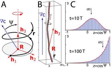
Figure 1: A. A helical path $\mathbf{r}$ can be described as the trajectory of a point on the circumference of a disk which rotates and translates; see text for details. B. Helical swimming path $\mathbf{r}$ of a chemotactic chiral swimmer in a linear concentration field: The helix vector $\mathbf{h}_{3}$ fluctuates around the direction of the concentration gradient $\bm{\nabla}c$. Parameters were $v_{0}=r_{0}/\sigma$, $\tau_{0}=0.2/r_{0}$, $-\kappa_{1}=\tau_{1}=0.5/r_{0}$, $\mu=\sigma$, $\lambda c_{0}=10^{2}/\sigma$, $|\mathbf{c}_{1}|=10^{-2}c_{0}/r_{0}$. C. Histograms of $z=\cos\psi$ where $\psi$ equals the angle enclosed by the helix axis and the gradient direction for a simulated ensemble of helical swimming paths as in B with initial distribution $P(z,0)=\delta(z)$ at times $t=10T,100T$. Also shown is the analytical solution $P(z,t)$ (red). Approximately, $P(z,100T)$ equals the steady-state distribution $P_{0}(z)\sim\exp({\rm Pe}\,z)$.

At steady state, a chemotactic chiral swimmer moves up a concentration gradient with average speed $\langle z\rangle\overline{v}$. The chemotaxis index $\rm CI$ is defined as the ratio of this average speed gradient-upwards and the swimming speed $v_{0}$

$${\rm CI}=\langle z\rangle{\rm CI_{max}},\quad{\rm CI_{max}}=\overline{v}/v_{0}=\sin\theta_{0}.$$ (15)

Note that ${\rm CI}$ approaches its maximal value $\rm CI_{max}$ for ${\rm Pe}\mathrel{\hbox to0.0pt{\lower 4.0pt\hbox{\hskip 1.0pt$\sim$}\hss}\raise 1.0pt\hbox{$>$}}1$. This condition is satisfied already beyond moderate concentration gradients with $|\bm{\nabla}c|\mathrel{\hbox to0.0pt{\lower 4.0pt\hbox{\hskip 1.0pt$\sim$}\hss}\raise 1.0pt\hbox{$>$}}|\varepsilon|/(\lambda r_{0})^{2}$. The maximal value $\rm CI_{max}$ for the chemotaxis index is limited only by the geometry of helical swimming.

Relation to experiments. Chemotaxis of sperm cells has been extensively studied for sea urchin sperm cells Kaupp et al. (2008). Tracking experiments in three dimensions show that these sperm cells swim along noisy helical paths with typical values for swimming speed, average curvature and torsion $v_{0}\approx 100-200\,\mu{\rm m}\,{\rm s}^{-1}$, $\kappa_{0}\approx 0.025-0.05\,\mu{\rm m}^{-1}$, $\tau_{0}\approx-0.0025\,\mu{\rm m}^{-1}$ Crenshaw (1996a); Corkidi et al. (2008). For comparision, the length of the sperm tail is ${L\approx 50\,\mu{\rm m}}$ Böhmer et al. (2005). Using a two-dimensional experimental setup in which sperm cells swim along a circular path, it has been shown that a periodic chemotactic stimulus causes a phase-locked periodic swimming response Böhmer et al. (2005); Wood et al. (2005). Such a behavioural response is consistent with our model of a chemotactic chiral swimmer.

In a pioneering experiment, C. J. Brokaw observed helical swimming paths of bracken fern sperm cells in a shallow observation chamber Brokaw (1958, 1959) . In the absence of chemoattractant, sperm swimming paths were noisy helices whose centerlines could be described as planar persistent random walks with persistence time $t_{P,\rm 2d}\approx 5\,{\rm s}$ and net speed $\overline{v}\approx 200\,{\mu\rm m}\,{\rm s}^{-1}$, corresponding to a persistence length of $l_{P,\rm 2d}\approx 1\,{\rm mm}$. Accordingly, the planar orientational fluctuations of the helix vector are characterized by a rotational diffusion coefficient $D=t_{P,\rm 2d}^{-1}=0.2\,{\rm s}^{-1}$. In a strong concentration gradient of chemoattractant, sperm swimming paths were bent helices which aligned with the gradient direction at a rate proportional to the relative strength of the concentration gradient $\beta\approx 150\,{\mu\rm m}\,{\rm s}^{-1}\,|\bm{\nabla}c|/c$ . In an initially homogeneous concentration field of charged chemoattractant, alignment of helical sperm swimming paths could also induced by applying an external electrical field $|\mathbf{E}|$. In this case, it was found that the alignment rate is proportional to the field strength $\beta/|\mathbf{E}|\approx 1.6\,{\rm s}^{-1}\,{\rm(V/cm)}^{-1}$. The mean alignment $\langle z\rangle=\langle\mathbf{h}_{3}\cdot\mathbf{E}\rangle/|\mathbf{E}|$ of helical paths at steady state was measured as a function of field strength $|\mathbf{E}|$. The experimental data could be well fitted by eqn. (14) assuming ${\rm Pe}\sim|\mathbf{E}|$ and yielded ${\rm Pe}/|\mathbf{E}|\approx 8\,{(\rm V/cm)}^{-1}$ . The above estimates for $D$ and $\beta/|\mathbf{E}|$ give approximately the same value for ${\rm Pe}/|\mathbf{E}|=(\beta/D)/|\mathbf{E}|$ Brokaw (1959). The physical origin of helix alignment in an electrical field is not entirely known: The observed alignment might be due to electrohydrodynamic effects resulting from sperm cells binding chemoattractant ions (with sperm cells effectively behaving as electric dipoles) Brokaw (1959). An alternative possibility is that the electric field induces a concentration gradient of chemoattractant ions and that the observed alignment of helical paths is a result of chemotactic navigation in this gradient.

Conclusion. In this Letter, we studied the stochastic differential geometry of noisy helical swimming paths which is relevant for many biological mircoswimmers with chiral propulsion Corkidi et al. (2008); Brokaw (1958, 1959); Crenshaw (1996a); Jennings (1901); Fenchel and Blackburn (1999); McHenry and Strother (2003); Jékely et al. (2008); Thar and Fenchel (2001). A simple feedback mechanism enables a chiral swimmer to navigate along a helical path upwards a concentration gradient of chemoattractant. Chemotaxis along noisy helices is employed by sperm cells and possbily other biological microswimmers Brokaw (1958, 1959); Crenshaw (1996a); Jennings (1901); Fenchel and Blackburn (1999); Thar and Fenchel (2001). A similar mechanism underlies phototaxis of the unicellular flagellate Chlamydomonas Crenshaw (1996b), and is found in phototactic marine zooplankton McHenry and Strother (2003); Jékely et al. (2008). Our theory shows that navigation along helical paths is remarkably robust in the presence of fluctuations: An effective rotation of the helix vector is determined by integrating its orientational fluctuations over several helical turns. Consequently, a small bias in these orientational fluctuations due to chemotactic signaling results in robust steering and the helix vector tends to align with the concentration gradient $\bm{\nabla}c$. If chemotactic signaling is adaptive, the alignment rate $\beta$ is proportional to the relative strength of the concentration gradient $|\bm{\nabla}c|/c$. After a transient period of alignment of duration $\beta^{-1}$, a chemotactic chiral swimmer moves upwards the concentration gradient with an average speed that is only limited by the geometry of helical swimming provided the strength of the concentration gradient exceeds a characteristic value. We conclude that temporal sampling of a concentration field along a helical path provides a universal strategy for chemotaxis which is highly adapted for a noisy environment.

References

- Purcell (1977) E. M. Purcell, Am. J. Phys. 45, 1 (1977).
- Lauga and Powers (2009) E. Lauga and T. R. Powers, Rep. Prog. Phys. ?, ? (2009), arXiv:0812.2887v1.
- Crenshaw (1993) H. C. Crenshaw, Bull. Math. Biol. 55, 197 (1993).
- Corkidi et al. (2008) G. Corkidi, B. Taboada, C. D. Wood, A. Guerrero, A. Darszon, Biochem. & Biophys. Res. Comm. 373, 125 (2008).
- Brokaw (1958) C. J. Brokaw, J. exp. Biol. 35, 197 (1958).
- Brokaw (1959) C. J. Brokaw, J. Cell. Comp. Physiol. 54, 95 (1959).
- Crenshaw (1996a) H. C. Crenshaw, Americ. Zool. 36, 608 (1996a).
- Jennings (1901) H. S. Jennings, Am. Soc. Natural. 35, 369 (1901).
- Fenchel and Blackburn (1999) T. Fenchel and N. Blackburn, Protist 150, 325 (1999).
- McHenry and Strother (2003) M. J. McHenry, J. A. Strother, Marine Biol. 142, 173 (2003).
- Jékely et al. (2008) G. Jékely, J. Colombelli, H. Hausen, K. Guy, E. Stelzer, F. Nédélec, and D. Arendt, Nature 456, 395 (2008).
- Thar and Fenchel (2001) R. Thar and T. Fenchel, Appl. Env. Microbiol. 67, 3299 (2001).
- Berg (2004) H. C. Berg, E. coli in Motion (Springer, 2004).
- Dusenbery (1997) D. B. Dusenbery, Proc. Natl. Acad. Sci. U.S.A. 94, 10949 (1997).
- Böhmer et al. (2005) M. Böhmer, Q. Van, I. Weyand, V. Hagen, M. Beyermann, M. Matsumoto, M. Hoshi, E. Hildebrand, and U. B. Kaupp, EMBO J. 24, 2741 (2005).
- Kaupp et al. (2008) U. B. Kaupp, N. D. Kashikar, and I. Weyand, Annu. Rev. Physiol. 70, 93 (2008).
- Crenshaw and Edelstein-Keshet (1993) H. C. Crenshaw and L. Edelstein-Keshet, Bull. Math. Biol. 55, 213 (1993).
- Friedrich and Jülicher (2007) B. M. Friedrich and F. Jülicher, Proc. Natl. Acad. Sci. U.S.A. 104, 13256 (2007).
- Kamien (2002) R. D. Kamien, Rev. Mod. Phys. 74, 953 (2002).
- Friedrich (2008) B. M. Friedrich, Phys. Biol. 5, 026007(6) (2008).
- Friedrich and Jülicher (2008) B. M. Friedrich and F. Jülicher, New J. Phys. 10, 123025(19) (2008).
- Barkai and Leibler (1997) N. Barkai and S. Leibler, Nature 387, 913 (1997).
- Debye (1929) P. J. W. Debye, Polar molecules (Dover, 1929).
- Wood et al. (2005) C. D. Wood, T. Nishigaki, T. Furuta, A. S. Baba, and A. Darszon, J. Cell. Biol. 169, 725 (2005).
- Crenshaw (1996b) H. C. Crenshaw, Mol. Biol. Cell. 7, 279 (1996b).