Pattern Formation, Social Forces, and Diffusion Instability in Games with Success-Driven Motion

Abstract

A local agglomeration of cooperators can support the survival or spreading of cooperation, even when cooperation is predicted to die out according to the replicator equation, which is often used in evolutionary game theory to study the spreading and disappearance of strategies. In this paper, it is shown that success-driven motion can trigger such local agglomeration and may, therefore, be used to supplement other mechanisms supporting cooperation, like reputation or punishment. Success-driven motion is formulated here as a function of the game-theoretical payoffs. It can change the outcome and dynamics of spatial games dramatically, in particular as it causes attractive or repulsive interaction forces. These forces act when the spatial distributions of strategies are inhomogeneous. However, even when starting with homogeneous initial conditions, small perturbations can trigger large inhomogeneities by a pattern-formation instability, when certain conditions are fulfilled. Here, these instability conditions are studied for the prisoner’s dilemma and the snowdrift game. Furthermore, it is demonstrated that asymmetrical diffusion can drive social, economic, and biological systems into the unstable regime, if these would be stable without diffusion.

1 Introduction

Game theory is a well-established theory of individual strategic interactions with applications in sociology, economics, and biology Neumann ; Axelrod ; Rapoport ; Gintis ; Binmore ; Nowak , and with many publications even in physics (see Ref. Network2 for an overview). It distinguishes different behaviors, so-called strategies $i$, and expresses the interactions of individuals in terms of payoffs $P_{ij}$. The value $P_{ij}$ quantifies the result of an interaction between strategies $i$ and $j$ for the individual pursuing strategy $i$. The more favorable the outcome of the interaction, the higher is the payoff $P_{ij}$.

There are many different games, depending on the structure of the payoffs, the social interaction network, the number of interaction partners, the frequency of interaction, and so on Gintis ; Binmore . Theoretical predictions for the selection of strategies mostly assume a rational choice approach, i.e. a payoff maximization by the individuals, although experimental studies Kagel ; Camerer ; Henrich support conditional cooperativity Conditional and show that moral sentiments Unselfish can support cooperation. Some models also take into account learning (see, e.g. Flache and references therein), where it is common to assume that more successful behaviors are imitated (copied). Based on a suitable specification of the imitation rules, it can be shown imit1 ; imit2 ; Kluwer that the resulting dynamics can be described by game-dynamical equations gamedyn1 ; gamedyn2 , which agree with replicator equations for the fitness-dependent reproduction of individuals in biology Eigen ; Fisher ; Schuster .

Another field where the quantification of human behavior in terms of mathematical models has been extremely successful concerns the dynamics of pedestrians molnar , crowds panic , and traffic tilch . The related studies have led to fundamental insights into observed self-organization phenomena such as stop-and-go waves tilch or lanes of uniform walking direction molnar . In the meantime, there are many empirical crowdturb and experimental results TranSci ; Hoogendoorn , which made it possible to come up with well calibrated models of human motion ACS3 ; Yu .

Therefore, it would be interesting to know what happens if game theoretical models are combined with models of driven motion. Would we also observe self-organization phenonomena in space and time? This is the main question addressed in this paper. Under keywords such as “assortment” and “network reciprocity”, it has been discussed that the clustering of cooperators can amplify cooperation, in particular in the prisoner’s dilemma Pepper ; cluster1 ; cluster2 ; cluster3 . Therefore, the pattern formation instability is of prime importance to understand the emergence of cooperation between individuals. In Sec. 4, we will study the instability conditions for the prisoner’s dilemma and the snowdrift game. Moreover, we will see that games with success-driven motion and asymmetrical diffusion may show pattern formation, where a homogeneous distribution of strategies would be stable without the presence of diffusion. It is quite surprising that sources of noise like diffusion can support the self-organization in systems, which can be described by game-dynamical equations with success-driven motion. This includes social, economic, and biological systems.

We now proceed as follows: In Sec. 2, we introduce the game-dynamical replicator equation for the prisoner’s dilemma (PD) and the snow-drift game (SD). In particularly, we discuss the stationary solutions and their stability, with the conclusion that cooperation is expected to disappear in the prisoner’s dilemma. In Sec. 3, we extend the game-dynamical equation by the consideration of spatial interactions, success-driven motion, and diffusion. Section 3.1 compares the resulting equations with reaction-diffusion-advection equations and discusses the similarities and differences with Turing instabilities and differential flow-induced chemical instabilities (DIFICI). Afterwards, Sec. 4 analyzes the pattern formation instability for the prisoner’s dilemma and the snowdrift game with its interesting implications, while details of the instability analysis are provided in Appendix B. Finally, Sec. 5 studies the driving forces of the dynamics in cases of large deviations from stationary and homogeneous strategy distributions, before Sec. 6 summarizes the paper and presents an outlook.

2 The Prisoner’s Dilemma without Spatial Interactions

In order to grasp the major impact of success-driven motion and diffusion on the dynamics of games (see Sec. 3), it is useful to investigate first the game-dynamical equations without spatial interactions. For this, we represent the proportion of individuals using a strategy $i$ at time $t$ by $p_{i}(t)$. While the discussion can be extended to any number of strategies, we will focus on the case of two strategies only for the sake of analytical tractability. Here, $i=1$ shall correspond to the cooperative strategy, $i=2$ to defection (cheating or free-riding). According to the definition of probabilities, we have $0\leq p_{i}(t)\leq 1$ for $i\in\{1,2\}$ and the normalization condition

$$p_{1}(t)+p_{2}(t)=1\,.$$ (1)

Let $P_{ij}$ be the payoff, if strategy $i$ meets strategy $j$. Then, the expected payoff for someone applying strategy $i$ is

$$E_{i}(t)=\sum_{j=1}^{2}P_{ij}p_{j}(t)\,,$$ (2)

as $p_{j}(t)$ represents the proportion of strategy $j$, with which the payoffs $P_{ij}$ must be weighted. The average payoff in the population of individuals is

$$\overline{E}(t)=\sum_{l=1}^{2}E_{l}(t)p_{l}(t)=\sum_{l=1}^{2}\sum_{j=1}^{2}p_{l}(t)P_{lj}p_{j}(t)\,.$$ (3)

In the game-dynamical equations, the temporal increase $dp_{i}(t)/dt$ of the proportion of individuals using strategy $i$ is proportional to the number of individuals pursuing strategy $i$ who may imitate, i.e. basically to $p_{i}(t)$. The proportionality factor, i.e. the growth rate $\lambda(i,t)$, is given by the difference between the expected payoff $E_{i}(t)$ and the average payoff $\overline{E}(t)$:

$$\frac{dp_{i}(t)}{dt} = \lambda(i,t)p_{i}(t)=\big{[}E_{i}(t)-\overline{E}(t)\big{]}p_{i}(t)$$ (4)

$$= \bigg{(}\sum_{j=1}^{2}P_{ij}p_{j}(t)-\sum_{l=1}^{2}\sum_{j=1}^{2}p_{l}(t)P_{lj}p_{j}(t)\bigg{)}p_{i}(t)\,.\quad$$

The equations (4) are known as replicator equations. They were originally developed in evolutionary biology to describe the spreading of “fitter” individuals through their higher reproductive success Eigen ; Fisher ; Schuster . However, the replicator equations were also used in game theory, where they are called “game-dynamical equations” gamedyn1 ; gamedyn2 . For a long time, it was not clear whether or why these equations could be applied to the frequency $p_{i}(t)$ of behavioral strategies, but it has been shown that the equations can be derived from Boltzmann-like equations for imitative pair interactions of individuals, if “proportional imitation” or similar imitation rules are assumed imit1 ; imit2 ; Kluwer .

Note that one may add a mutation term to the right-hand side of the game-dynamical equations (4). This term could, for example, be specified as

$$W_{2}p_{2}(t)-W_{1}p_{1}(t) = rq[1-p_{1}(t)]-r(1-q)p_{1}(t)$$ (5)

$$= r[q-p_{1}(t)]$$

for strategy $i=1$, and by the negative expression of this for $i=2$. Here, $r$ is the overall mutation rate, $W_{2}=rq$ the mutation rate towards cooperation, and $W_{1}=r(1-q)$ the mutation rate towards defection Kluwer . This implementation reflects spontaneous, random strategy choices due to erroneous or exploration behavior and modifies the stationary solutions.

It can be shown that

$$\sum_{i=1}^{2}\frac{dp_{i}(t)}{dt}=0\,,$$ (6)

so that the normalization condition (1) is fulfilled at all times $t$, if it is fulfilled at $t=0$. Moreover, the equation $dp_{i}(t)/dt=\lambda p_{i}(t)$ implies $p_{i}(t)\geq 0$ at all times $t$, if $p_{i}(0)\geq 0$ for all strategies $i$.

We may now insert the payoffs of the prisoner’s dilemma, i.e.

$$P_{11} = R\mbox{ (``reward''),}$$

$$P_{12} = S\mbox{ (``sucker's payoff''),}$$

$$P_{21} = T\mbox{ (``temptation''), and}$$

$$P_{22} = P\mbox{ (``payoff'')}$$ (7)

with the assumed payoff relationships

$$T>R>P>S\,.$$ (8)

Additionally, one often requires

$$2R>S+T\,.$$ (9)

The “reward” $R$ is the payoff for mutual cooperation and the “punishment” $P$ the payoff for mutual defection, while $T$ is the “temptation” of unilateral defection, and a cheated cooperator receives the sucker’s payoff $S$. While we have $P>S$ in the prisoner’s dilemma, the snowdrift game (also known as chicken or hawk-dove game) is characterized by $S>P$, i.e. it is defined by

$$T>R>S>P\,.$$ (10)

Both games are characterized by a temptation to defect ($T>R$), while the prisoner’s dilemma has the additional challenge that there is a high risk to cooperate ($S<P$). This difference has a large influence on the resulting level $p_{1}(t)$ of cooperation: Inserting the above payoffs into Eq. (4), one eventually obtains the game-dynamical equation

$$\frac{dp_{1}(t)}{dt}=[1-p_{1}(t)]\big{[}-A+Bp_{1}(t)\big{]}p_{1}(t)\,.$$ (11)

This directly follows from Eq. (46) of Appendix A, when the abbreviations

$$A=P-S\qquad\mbox{and}\qquad B=P+R-S-T$$ (12)

are used to pronounce the equation’s structure. Setting $dp_{1}(t)/dt=0$, one obviously finds three stationary solutions $p_{1}(t)=p_{1}^{k}$, namely

$$p_{1}^{1}=0\,,\quad p_{1}^{2}=1\,\quad\mbox{and}\quad p_{1}^{3}=\frac{A}{B}\,.$$ (13)

Not all of these solutions are stable with respect to small deviations. In fact, a linear stability analysis (see Appendix A) delivers the eigenvalues

$$\lambda_{1}=-A,\qquad\lambda_{2}=A-B,\qquad\mbox{and}\qquad\lambda_{3}=A\left(1-\frac{A}{B}\right).$$ (14)

The stationary solution $p_{1}^{k}$ is stable with respect to perturbations (i.e. small deviations from them), if $\lambda_{k}\leq 0$, while for $\lambda_{k}>0$, the deviation will grow in time. Due to

$$A-B=T-R>0\,,$$ (15)

the solution $p_{1}^{2}=1$ corresponding to 100% cooperators is unstable with respect to perturbations, i.e. it will not persist. Moreover, the solution $p_{1}^{1}$ will be stable in the prisoner’s dilemma because of $A=P-S>0$. This corresponds to 0% cooperators and 100% defectors, which agrees with the expected result for the one-shot prisoner’s dilemma (if individuals decide according to rational choice theory). In the snowdrift game, however, the stationary solution $p_{1}^{1}=0$ is unstable due to $A=P-S<0$, while the additional stationary solution $p_{1}^{3}=A/B<1$ is stable. Hence, in the snowdrift game with $B<A<0$, we expect the establishment of a fraction $A/B$ of cooperators. For the prisoner’s dilemma, the solution $p_{1}^{3}$ does not exist, as it does not fall into the range between 0 and 1 that is required from probabilities: If $B>0$, we have $p_{1}^{3}=A/B>1$, while $p_{1}^{3}=A/B<0$ for $B<0$.

In summary, for the prisoner’s dilemma, there is no evolutionarily stable solution with a finite percentage of cooperators, if we do not consider spontaneous strategy mutations (and neglect the effect of spatial correlations through the applied factorization assumption). According to the above, cooperation in the PD is essentially expected to disappear. Strategy mutations, of course, can increase the stable level $p_{1}^{1}$ of cooperation from zero to a finite value. Specifically, $p_{1}^{1}$ will assume a value close to zero for small values of $r$, while it will converge to $q$ in the limit $r\rightarrow\infty$.

In the next section, we will show that

1. when the proportions of cooperators and defectors are allowed to vary in space, i.e. if the distribution of cooperators and defectors is inhomogeneous, the proportion of cooperators may locally grow,

2. we obtain such a variation in space by success-driven motion, as it can destabilize a homogeneous distribution of strategies, which gives rise to spatial pattern formation in the population (agglomeration or segregation or both EPL ).

Together with the well-known fact that a clustering of cooperators can promote cooperation Pepper ; cluster1 ; cluster2 ; cluster3 , pattern formation can potentially amplify the level of cooperation, as was demonstrated numerically for a somewhat related model in Ref. ACS5 . We will also show that, in contrast to success-driven motion, random motion (“diffusion” in space) stabilizes the stationary solution $p_{1}^{1}$ with 0% cooperators (or, in the presence of strategy mutations, with a small percentage of cooperators).

3 Taking into Account Success-Driven Motion and Diffusion in Space

We now assume that individuals are distributed over different locations $x\in[0,L]$ of a one-dimensional space. A generalization to multi-dimensional spaces is easily possible. For the sake of simplicity, we assume that the spatial variable $x$ is scaled by the spatial extension $L$, so that $x$ is dimensionless and varies between 0 and 1. In the following, the proportion of individuals using strategy $i$ at time $t$ and at a location between $x$ and $x+dx$ is represented by $p_{i}(x,t)dx$ with $p_{i}(x,t)\geq 0$. Due to the spatial degrees of freedom, the proportion of defectors is not immediately given by the the proportion of cooperators anymore, and the previous normalization condition $p_{2}(t)=1-p_{1}(t)$ is replaced by the less restrictive condition

$$\sum_{i=1}^{2}\int\limits_{0}^{L}dx\,p_{i}(x,t)=1\,.$$ (16)

This allows the fractions of cooperators and defectors to uncouple locally, i.e. the proportion of cooperators does not have to decrease anymore by the same amount as the proportion of defectors increases.

Note that, if $\rho_{i}(x,t)=p_{i}(x,t)N/L$ represents the density of individuals pursuing strategy $i$ at location $x$ and time $t$, Eq. (16) can be transferred into the form

$$\sum_{i=1}^{2}\int\limits_{0}^{1}dx\,\rho_{i}(x,t)=\frac{N}{L}=\rho\,,$$ (17)

where $N$ is the total number of individuals in the system and $\rho$ their average density.

One may also consider to treat unoccupied space formally like a third strategy $i=0$. In this case, however, the probabilities $p_{i}(x,t)$ in all locations $x$ add up to the maximum concentration $p_{\rm max}$, see Eq. (23). This means

$$p_{0}(x,t)=p_{\rm max}-p_{1}(x,t)-p_{2}(x,t)$$ (18)

and

$$\frac{\partial p_{0}(x,t)}{\partial t}=-\frac{\partial p_{1}(x,t)}{\partial t}-\frac{\partial p_{2}(x,t)}{\partial t}\,.$$ (19)

Therefore, $p_{0}(x,t)$ can be eliminated from the system of equations, because unoccupied space does not interact with strategies 1 and 2. As a consequence, the dynamics in spatial games with success-driven motion is different from the cyclic dynamics in games considering volunteering volun : In order to survive invasion attempts by defectors in the prisoner’s dilemma, one could think that cooperators would seek separated locations, where they would be “loners”. However, cooperators do not tend to maneuver themselves into non-interactive states ACS5 : On the contrary: The survival of cooperators rather requires to have a larger average number of interaction partners than defectors have.

After this introductory discussion, let us now extend the game-dynamical equations according to

$$\frac{\partial p_{i}(x,t)}{\partial t} = \bigg{(}\sum_{l=1}^{2}p_{l}\sum_{j=1}^{2}P_{ij}p_{j}-\sum_{l=1}^{2}\sum_{j=1}^{2}p_{l}P_{lj}p_{j}\bigg{)}p_{i}(x,t)$$ (20)

$$- \frac{\partial}{\partial x}\left(p_{i}(x,t)\frac{\partial E_{i}(x,t)}{\partial x}\right)+D_{i}\frac{\partial^{2}p_{i}(x,t)}{\partial x^{2}}\qquad$$

with the local expected success

$$E_{i}(x,t)=\sum_{j=1}^{2}P_{ij}p_{j}(x,t)\,,$$ (21)

compare Eq. (2). The additional sum $\sum_{l}p_{l}$ had to be introduced for reasons of normalization, as we do not have $p_{1}+p_{2}=1$ any longer. $\partial p_{i}(x,t)/\partial t$ represents the (partial) time derivative. The first term in large brackets on the right-hand side of Eq. (20) assumes that locally, an imitation of more successful strategies occurs. An extension of the model to interactions with neighboring locations would be easily possible. The second term, which depends on $E_{i}(x,t)$, describes success-driven motion withTamas ; withTadek . Finally, the last term represents diffusion, and $D_{i}\geq 0$ are called diffusion coefficients or diffusivities. These terms can be generalized to multi-dimensional spaces by replacing the spatial derivative $\partial/\partial x$ by the nabla operator $\vec{\nabla}$.

The notion of success-driven motion is justified for the following reason: Comparing the term describing success-driven motion with a Fokker-Planck equation FPG , one can conclude that it corresponds to a systematic drift with speed

$$V_{i}(x,t)=\frac{\partial E_{i}(x,t)}{\partial x}\,.$$ (22)

According to this, individuals move into the direction of the gradient of the expected payoff, i.e. the direction of the (greatest) increase of $E_{i}(x,t)$. In order to take into account capacity constraints (saturation effects), one could introduce a prefactor

$$C(x,t)=1-\sum_{l=1}^{2}\frac{p_{l}(x,t)N}{\rho_{\rm max}L}\geq 0\,,$$ (23)

where $\rho_{\rm max}=p_{\rm max}N/L\geq N/L>0$ represents the maximum density of individuals. This would have to be done in the imitation-based replicator terms in the first line of Eq. (20) as well. In the following, however, we will focus on the case $C=1$, which allows for a local accumulation of individuals.

The last term in Eq. (20) is a diffusion term which reflects effects of random motion in space FPG . It can be easily seen that, for $D_{i}>0$, the diffusion term has a smoothing effect: It eventually reduces the proportion $p_{i}(x,t)$ in places $x$ where the second spatial derivative $\partial^{2}p_{i}/\partial x^{2}$ is negative, in particular in places $x$ where the distribution $p_{i}(x,t)$ has maxima in space. In contrast, the proportion $p_{i}(x,t)$ increases in time, where $\partial^{2}p_{i}/\partial x^{2}>0$, e.g. where the distribution has its minima. Assuming an additional smoothing term

$$D_{0}\,\frac{\partial^{4}p_{i}(x,t)}{\partial x^{4}}$$ (24)

with a small constant $D_{0}>0$ on the right-hand side of Eq. (20) makes the numerical solution of this model well-behaved (see Appendix B).

When Eq. (20) is solved, one may, for example, assume periodic boundary conditions (i.e. a circular space). In this case, we have $p_{i}(1,t)=p_{i}(0,t)$ and $\partial^{k}p_{i}(1,t)/\partial x^{k}=\partial^{k}p_{i}(0,t)/\partial x^{k}$, and by means of partial integration, it can be shown that

$$\frac{\partial}{\partial t}\sum_{i=1}^{2}\int\limits_{0}^{1}dx\,p_{i}(x,t)=0\,.$$ (25)

Therefore, Eq. (20) fulfils the normalization condition (16) at all times, if it is satisfied at $t=0$. Furthermore, it can be shown that $p_{i}(x,t)\geq 0$ for all times $t$, if this is true at time $t=0$ for all strategies $i$ and locations $x$.

3.1 Comparison with Reaction-Diffusion-Advection Equations

It is noteworthy that the extended game-dynamical model (20) has some similarity with reaction-diffusion-advection (RDA) equations. These equations have been developed to describe the dynamics of chemical reactions with spatial gradients, considering the effects of differential flows and diffusion. Specifically, the kinetics of (binary) chemical reactions is reflected by non-linear terms similar to those in the first line on the right-hand side of Eq. (20). The first term in the second line represents advection terms (differential flows), while the last term of Eq. (20) delineates diffusion effects.

Considering this apparent similarity, what dynamics do we expect? It is known that reaction-diffusion equations can show a Turing instability Turing1 ; Turing3 (also without an advection term). Specifically, for a chemical activator-inhibitor system, one can find a linearly unstable dynamics, if the diffusivities $D_{1}$ and $D_{2}$ are different. As a consequence, the concentration of chemicals in space will be non-homogeneous. This effect has been used to explain pattern formation processes in morphogenesis Meinhardt ; Turing2 . Besides the Turing instability, a second pattern-forming instability can occur when chemical reactions are coupled with differential flows. These so-called “differential flow-induced chemical instabilities” (DIFICI) can occur even for equal or vanishing diffusivities $D_{i}=D$, but they may also interact with the Turing instability DIF1 ; DIF2 ; DIF3 ; DIF4 ; DIF5 .

The difference of the extended game-dynamical equation (20) as compared to the RDA equations lies in the specification of the velocity $V_{i}(x,t)$, which is determined by the gradient of the expected success $E_{i}(x,t)$. Therefore, the advective term is self-generated by the success of the players. We may rewrite the corresponding term in Eq. (20) as follows:

$$-\frac{\partial}{\partial x}\left(p_{i}\frac{\partial E_{i}}{\partial x}\right)=-\sum_{j=1}^{2}P_{ij}\frac{\partial p_{i}}{\partial x}\frac{\partial p_{j}}{\partial x}-\sum_{j=1}^{2}p_{i}P_{ij}\frac{\partial^{2}p_{j}}{\partial x^{2}}\,.$$ (26)

According to the last term of this equation, the advection term related to success-driven motion implies effects similar to a diffusion term with negative diffusion coefficients $p_{i}P_{ij}$ (if $P_{ij}>0$). Additionally, there is a non-linear dependence on the gradients $\partial p_{i}/\partial x$ and $\partial p_{j}/\partial x$ of the strategy distributions in space. Both terms couple the dynamics of different strategies $j$.

As a consequence of this, the resulting instability conditions and dynamics are different from the RDA equations. We will show that, without success-driven motion, diffusion cannot trigger pattern formation. Diffusion rather counteracts spatial inhomogeneities. Success-driven motion, in contrast, causes pattern formation in a large area of the parameter space of payoffs, partly because of a negative diffusion effect.

Besides this, we will show that different diffusivities $D_{i}$ may trigger a pattern formation instability in case of payoff parameters, for which success-driven motion does not destabilize homogeneous strategy distributions in the absence of diffusion. This counter-intuitive effect reminds of the Turing instability, although the underlying mathematical model is different, as pointed out before. In particular, the largest growth rate does not occur for finite wave numbers, as Appendix B shows. The instability for asymmetric diffusion is rather related to the problem of “noise-induced transitions” in systems with multiplicative noise, which are characterized by space-dependent diffusion coefficients Horsthemke . A further interesting aspect of success-driven motion is the circumstance that the space-dependent diffusion effects go back to binary interactions, as the multiplicative dependence on $p_{i}$ and $p_{j}$ shows.

4 Linear Instability of the Prisoner’s Dilemma and the Snowdrift Game

After inserting the payoffs (7) of the prisoner’s dilemma and the snowdrift game into Eq. (20), one can see the favorable effect on the spreading of cooperation that the spatial dependence, in particular the relaxed normalization condition (16) can have: For $i=1$, Eq. (20) becomes

$$\frac{\partial p_{1}(x,t)}{\partial t} = p_{2}\Big{[}(R-T)p_{1}+(S-P)p_{2}\Big{]}p_{1}$$ (27)

$$+ \frac{\partial}{\partial x}\left[(D_{1}-p_{1}R)\frac{\partial p_{1}}{\partial x}-p_{1}S\frac{\partial p_{2}}{\partial x}\right]\,.\qquad$$

It is now an interesting question, whether the agglomeration of cooperators can be supported by success-driven motion. In fact, the second line of Eq. (27) can be rewritten as

$$(D_{1}-p_{1}R)\frac{\partial^{2}p_{1}}{\partial x^{2}}-R\left(\frac{\partial p_{1}}{\partial x}\right)^{2}\!-p_{1}S\frac{\partial^{2}p_{2}}{\partial x^{2}}-S\frac{\partial p_{1}}{\partial x}\,\frac{\partial p_{2}}{\partial x}\,.$$ (28)

This shows that a curvature $\partial^{2}p_{i}/\partial x^{2}<0$ can support the increase of the proportion of strategy $i$ as compared to the game-dynamical equation (4) without spatial dependence. The situation becomes even clearer, if a linear stability analysis of Eqs. (27) is performed (see Appendix B). The result is as follows: If the square of the wave number $\kappa$, which relates to the curvature of the strategy distribution, is large enough (i.e. if the related cluster size is sufficiently small), the replicator terms in the first line on the right-hand side of equation (20) become negligible. Therefore, the conditions, under which homogeneous initial strategy distributions $p_{i}^{0}$ are linearly unstable, simplify to

$$p_{1}^{0}R+p_{2}^{0}P>D_{1}+D_{2}$$ (29)

and

$$(p_{1}^{0}R-D_{1})(p_{2}^{0}P-D_{2})<p_{1}^{0}p_{2}^{0}ST\,,$$ (30)

see Eqs. (74) and (75).

If condition (29) or condition (30) is fulfilled, we expect emergent spatio-temporal pattern formation, basically agglomeration or segregation or both EPL . As has been pointed out before, the agglomeration of cooperators can increase the level of cooperation. This effect is not possible, when spatial interactions are neglected. In that case, we stay with Eq. (11), and the favorable pattern-formation effect cannot occur.

Let us now discuss a variety of different cases:

1. In case of diffusive motion only (i.e. no success-driven motion), Eq. (29) must be replaced by

   $$0>D_{1}+D_{2}$$ (31)

   and Eq. (30) by

   $$D_{1}D_{2}<0\,,$$ (32)

   which cannot be fulfilled. Therefore, diffusion without success-driven motion does not support pattern formation or a related increase in the level of cooperation.

2. In the case of success-driven motion with finite diffusion, Eqs. (29) and (30) imply

   $$p_{1}^{0}R+(1-p_{1}^{0})P>D_{1}+D_{2}$$ (33)

   and

   $$(p_{1}^{0}R-D_{1})\big{[}(1-p_{1}^{0})P-D_{2}\big{]}<p_{1}^{0}(1-p_{1}^{0})ST\,,$$ (34)

   if the normalization condition $p_{2}^{0}=1-p_{1}^{0}$ for a homogeneous initial condition is taken into account. These instability conditions hold for both, the prisoner’s dilemma and the snowdrift game. Inequality (33) basically says that, in order to find spontaneous pattern formation, the agglomerative tendency $R$ of cooperators or the agglomerative tendency $P$ of defectors (or both) must be larger than the diffusive tendency. This agglomeration, of course, requires the reward $R$ of cooperation to be positive, otherwise cooperators would not like to stay in the same location. The alternative instability condition (34) requires that the product $RP$ of the payoffs resulting when individuals of the same strategy meet each other is smaller than the product $ST$ of payoffs resulting when individuals with different strategies meet each other. This basically excludes a coexistence of the two strategies in the same location and is expected to cause segregation. It is noteworthy that condition (34) is not invariant with respect to shifts of all payoffs $P_{ij}$ by a constant value $c$, in contrast to the replicator equations (46).

3. In case of the prisoner’s dilemma without strategy mutations, the stable stationary solution for the case without spontaneous strategy changes is $p_{1}^{0}=p_{1}^{1}=0$. This simplifies the instability conditions further, yielding

   $$P>D_{1}+D_{2}$$ (35)

   and

   $$-D_{1}(P-D_{2})<0\,.$$ (36)

   In order to fulfil one of these conditions, the punishment $P$ must be positive and larger than $D_{2}$ to support pattern formation (here: an aggregation of defectors). Naturally, the survival or spreading of cooperators requires the initial existence of a finite proportion $p_{1}^{0}>0$ of them, see the previous case.

4. In the special case $P=S=0$ ACS5 , Eqs. (33) and (34) become

   $$p_{1}^{0}R>D_{1}+D_{2}$$ (37)

   and

   $$-(p_{1}^{0}R-D_{1})D_{2}<0\,,$$ (38)

   which requires $p_{1}^{0}R>D_{1}$. Therefore, a finite initial proportion $p_{1}^{0}$ of cooperators is needed again for pattern formation (an agglomeration of cooperators). This can be easily reached by spontaneous strategy changes.

5. Neglecting diffusion for a moment (i.e. setting $D_{1}=D_{2}=0$), no pattern formation should occur, if the condition

   $$RP>ST$$ (39)

   and, at the same time,

   $$p_{1}^{0}R+(1-p_{1}^{0})P<0$$ (40)

   is fulfilled. Equation (39) implies the stability condition

   $$S<\frac{RP}{T}\,.$$ (41)

   Besides $T>R$, we have to consider here that $S<P$ in the prisoner’s dilemma and $S>P$ in the snowdrift game (see Fig. 1).

6. Finally, let us assume that the stability conditions $ST-RP<0$ and $p_{1}^{0}R+(1-p_{1}^{0})P<0$ for the previous case without diffusion ($D_{1}=D_{2}=0$) are fulfilled, so that no patterns will emerge. Then, depending on the parameter values, the instability condition following from Eq. (34),

   $$-(D_{1}-D_{2})\underbrace{(1-p_{1}^{0})}_{\geq 0}P$$ (42)

   $$< \underbrace{D_{2}}_{\geq 0}\underbrace{[p_{1}^{0}R+(1-p_{1}^{0})P]}_{<0}$$

   $$\underbrace{-D_{1}D_{2}}_{\leq 0}+\underbrace{p_{1}^{0}(1-p_{1}^{0})}_{\geq 0}\underbrace{(ST-RP)}_{<0}\,,\qquad$$

   may still be matched, if $(D_{1}-D_{2})$ is sufficiently large. Therefore, aymmetrical diffusion ($D_{1}\neq D_{2}$) can trigger a pattern formation instability, where the spatio-temporal strategy distribution without diffusion would be stable. The situation is clearly different for symmetrical diffusion with $D_{1}=D_{2}$, which cannot support pattern formation.

   Although the instability due to asymmetrical diffusion reminds of the Turing instability, it must be distinguished from it (see Sec. 3.1). So, how can the instability then be explained? The reason for it may be imagined as follows: In order to survive and spread, cooperators need to be able to agglomerate locally and to invade new locations. While the first requirement is supported by success-driven motion, the last one is promoted by a larger diffusivity $D_{1}>D_{2}$ of cooperators.

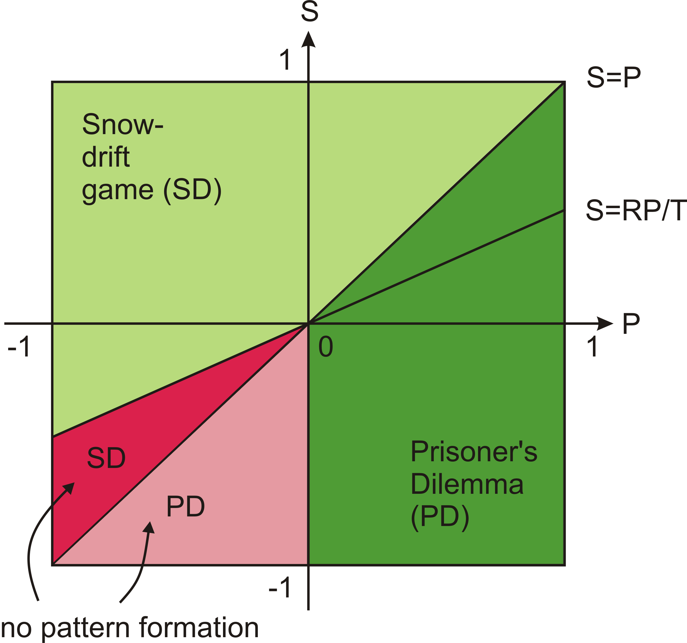
Figure 1: Payoff-dependence of pattern-formation in the prisoner’s dilemma with $S<P$ and the snowdrift game with $S>P$ according to a linear stability analysis for spatial games with success-driven motion, but no diffusion, strategy mutations, or noise. One can clearly see that spontaneous pattern-formation prevails (green area), and that there is only a small area for $P<0$ (marked red), where a homogeneous initial condition is stable with respect to small perturbations.

5 Social Forces in Spatial Games with Success-Driven Motion

In the previous section, we have shown how success-driven motion destabilizes homogeneous strategy distributions in space. This analysis was based on the study of linear (in)stability (see Appendix B). But what happens, when the deviation from the homogeneous strategy distribution is large, i.e. the gradients $\partial p_{i}/\partial x$ are not negligible any longer? This can be answered by writing Eq. (22) explicitly, which becomes

$$V_{i}(x,t)=\sum_{j=1}^{2}P_{ij}\frac{\partial p_{j}(x,t)}{\partial x}=\sum_{j=1}^{2}f_{ij}(x,t)\,.$$ (43)

Here, the expression

$$f_{ij}(x,t)=P_{ij}\frac{\partial p_{j}(x,t)}{\partial x}$$ (44)

(which can be extended by saturation effects), may be interpreted as interaction force (“social force”) excerted by individuals using strategy $j$ on an individual using strategy $i$. It is visible that the sign of $P_{ij}$ determines the character of the force. The force is attractive for positive payoffs $P_{ij}>0$ and repulsive for negative payoffs $P_{ij}<0$. The direction of the force, however, is determined by spatial changes $\partial p_{j}(x,t)/\partial x$ in the strategy distribution $p_{j}(x,t)$ (i.e. not by the strategy distribution itself).

It is not the size of the payoffs $P_{ij}$ which determines the strength of the interaction force, but the payoff times the gradient of the distribution of the strategy $j$ one interacts with (and the availability and reachability of more favorable neighboring locations, if the saturation prefactor $C$ is taken into account). Due to the dependence on the gradient $\partial p_{j}(x,t)/\partial x$, the impact of a dispersed strategy $j$ on individuals using strategy $i$ is negligible. This particularly applies to scenarios with negative self-interactions ($P_{jj}<0$).

Note that success-driven motion may be caused by repulsion away from the current location or by attraction towards more favorable neighborhoods. In the prisoner’s dilemma, for example, cooperators and defectors feel a strong attraction towards areas with a higher proportion of cooperators. However, cooperators seek each other mutually, while the attraction between defectors and cooperators is weaker. This is due to $T+S<2R$, see inequality (9). As a result, even if $P>0$, cooperators are moving away from defectors due to $R>P$ in order to find more cooperative locations, while defectors are following them.

Another interesting case is the game with the payoffs $P_{11}=P_{22}=-P$ and $P_{12}=P_{21}=Q>P$, where we have negative self-interactions among identical strategies and positive interactions between different strategies. Simulations for the no-imitation case show that, despite of the dispersive tendency of each strategy, strategies tend to agglomerate in certain locations thanks to the stronger attractive interactions between different strategies (see Fig. 3 in Ref. withTadek ).

The idea of social forces is long-standing. Montroll used the term to explain logistic growth laws Montroll , and Lewin introduced the concept of social fields to the social sciences in analogy to electrical fields in physics Lewin . However, a formalization of a widely applicable social force concept was missing for a long time. In the meantime, social forces were successfully used to describe the dynamics of interacting vehicles tilch or pedestrians molnar , but there, the attractive or repulsive nature was just assumed. Attempts to systematically derive social forces from an underlying decision mechanism were based on direct pair interactions in behavioral spaces (e.g. opinion spaces), with the observation that imitative interactions or the readiness for compromises had attrative effects Kluwer ; MatSoc . Here, for the first time, we present a formulation of social forces in game-theoretical terms. Considering the great variety of different games, depending on the respective specification of the payoffs $P_{ij}$, this is expected to find a wide range of applications, in particular as success-driven motion has been found to produce interesting and relevant pattern formation phenomena withTadek ; ACS5 .

6 Summary, Discussion, and Outlook

In this paper, we have started from the game-dynamical equations (replicator equation), which can be derived from imitative pair interactions between individuals imit1 ; imit2 . It has been shown that no cooperation is expected in the prisoner’s dilemma, if no spontaneous strategy mutations are taken into account, otherwise there will be a significant, but usually low level of cooperation. In the snowdrift game, in contrast, the stationary solution corresponding to no cooperation is unstable, and there is a stable solution with a finite level of cooperation.

These considerations have been carried out to illustrate the major difference that the introduction of spatial interactions based on success-driven motion and diffusion makes. While diffusion itself tends to support homogeneous strategy distributions rather than pattern formation, success-driven motion implies an unstable spatio-temporal dynamics under a wide range of conditions. As a consequence, small fluctations can destabilize a homogeneous distribution of strategies. Under such conditions, the formation of emergent patterns (agglomeration, segregation, or both) is expected. The resulting dynamics may be understood in terms of social forces, which have been formulated here in game-theoretical terms.

The destabilization of homogeneous strategy distributions and the related occurence of spontaneous pattern formation has, for example, a great importance for the survival and spreading of cooperators in the prisoner’s dilemma. While this has been studied numerically in the past ACS5 , future work based on the model of this paper and extensions of it shall analytically study conditions for the promotion of cooperation. For example, it will be interesting to investigate, how relevant the imitation of strategies in neighboring locations is, how important is the rate of strategy changes as compared to location changes, and how crucial is a territorial effect (i.e. a limitation $p_{\rm max}$ of the local concentration of individuals, which may protect cooperators from invasion by defectors).

Of course, instead of studying the continuous game-dynamical model with success-driven motion and calculating its instability conditions, one can also perform agent-based simulations for a discretized version of the model. For the case without imitation of superior strategies and symmetrical payoffs ($P_{ij}=P_{ji}$), it has been shown that the analytical instability conditions surprisingly well predict the parameter areas of the agent-based model, where pattern-formation takes place EPL . Despite the difference in the previously studied model (see footnote 2), this is also expected to be true for the non-symmetrical games studied here, in particular as we found that the influence of imitation on the instability condition is negligible, if the wave number $\kappa$ characterizing inhomogeneities in the initial distribution is large. This simplified the stability analysis a lot. Moreover, it was shown that asymmetrical diffusion can drive our game-theoretical model with success-driven motion from the stable regime into the unstable regime. While this reminds of the Turing instability Turing1 , it is actually different from it: Compared to reaction-diffusion-advection equations, the equations underlying the game-dynamical model with success-driven motion belong to another mathematical class, as is elaborated in Sec. 3.1.

In Sec. 5, it was pointed out that, in the prisoner’s dilemma, cooperators evade defectors, who seek cooperators. Therefore, some effects of success-driven motion (leaving unfavorable neighborhoods) may be interpreted as punishment of the previous interaction partners, who are left behind with a lower overall payoff. However, “movement punishment” of defectors by leaving unfavorable environments is different from the “costly” or “altruistic punishment” discussed in the literature Punish : In the strict sense, success-driven motion neither imposes costs on a moving individual nor on the previous interaction partners. If we would introduce a cost of movement, it would have to be paid by both, cooperators who evade defectors, and defectors who follow them. Therefore, costly motion would be expected to yield similar results as before, but it would still be different from altruistic punishment. It should also be pronounced that, besides avoiding unfavorable locations, success-driven motion implies the seeking of favorable environments, which has nothing to do with punishment. Without this element, e.g. when individuals leave unfavorable locations based on a random, diffusive motion, success-driven motion is not effective in promoting cooperation. Therefore, the mechanism of success-driven motion, despite some similar features, is clearly to be distinguished from the mechanism of punishment.

Finally, note that migration may be considered as one realization of success-driven motion. Before, the statistics of migration behavior was modeled by the gravity law gravity1 ; gravity2 or entropy approaches entropy1 ; entropy2 , while its dynamics was described by partial differential equations part1 ; part2 and models from statistical physics Weidlich . The particular potential of the approach proposed in this paper lies in the integration of migration into a game-theoretical framework, as we formalize success-driven motion in terms of payoffs and strategy distributions in space and time. Such integrated approaches are needed in the social sciences to allow for consistent interpretations of empirical findings within a unified framework.

Acknowledgments

The author would like to thank Peter Felten for preparing Fig. 1 and Christoph Hauert for comments on manuscript ACS5 .

Appendix A Linear Stability Analysis of the Game-Dynamical Equation Without Spatial Interactions

Inserting the payoffs (7) of the prisoner’s dilemma or the snowdrift game into Eq. (4), we get the game-dynamical equation

$$\frac{dp_{1}(t)}{dt} = \big{[}Rp_{1}+Sp_{2}-R(p_{1})^{2}$$ (45)

$$- (S+T)p_{1}p_{2}-P(p_{2})^{2}\big{]}p_{1}(t)\,.$$

Considering Eq. (1), i.e. $p_{2}(t)=1-p_{1}(t)$, we find

$$\frac{dp_{1}}{dt} = \big{[}Rp_{1}+S(1-p_{1})-R(p_{1})^{2}$$ (46)

$$-(S+T)p_{1}(1-p_{1})-P(1-p_{1})^{2}\big{]}p_{1}(t)$$

$$= (1-p_{1})\big{[}(S-P)+(P+R-S-T)p_{1}\big{]}p_{1}(t)\,.\qquad$$

This is a mean-value equation, which assumes a factorization of joint probabilities, i.e. it neglects correlations Kluwer . Nevertheless, the following analysis is suited to provide insights into the dynamics of the prisoner’s dilemma and the snowdrift game. Introducing the useful abbreviations

$$A=P-S\qquad\mbox{and}\qquad B=P+R-S-T,$$ (47)

Eq. (46) can be further simplified, and we get

$$\frac{dp_{1}(t)}{dt}=[1-p_{1}(t)]\big{[}-A+Bp_{1}(t)\big{]}p_{1}(t)\,.$$ (48)

Obviously, shifting all payoffs $P_{ij}$ by a constant value $c$ does not change Eq. (11), in contrast to the case involving spatial interactions discussed later.

Let $p_{1}^{k}$ with $k\in\{1,2,3\}$ denote the stationary solutions (13) of Eq. (11), defined by the requirement $dp_{1}/dt=0$. In order to analyze the stability of these solutions with respect to small deviations

$$\delta p_{1}(t)=p_{1}(t)-p_{1}^{k}\,,$$ (49)

we perform a linear stability analysis in the following. For this, we insert Eq. (49) into Eq. 11), which yields

$$\frac{d\delta p_{1}(t)}{dt} = (1-p_{1}^{k}-\delta p_{1})(-A+Bp_{1}^{k}+B\,\delta p_{1})(p_{1}^{k}+\delta p_{1})$$ (50)

$$= \big{[}(1-p_{1}^{k})p_{1}^{k}+(1-2p_{1}^{k})\delta p_{1}-(\delta p_{1})^{2}\big{]}$$

$$\times (-A+Bp_{1}^{k}+B\,\delta p_{1})\,.$$

If we concentrate on sufficiently small deviations $\delta p_{1}(t)$, terms containing factors $[\delta p_{1}(t)]^{m}$ with an integer exponent $m>1$ can be considered much smaller than terms containing a factor $\delta p_{1}(t)$. Therefore, we may linearize the above equations by dropping higher-order terms proportionally to $[\delta p_{1}(t)]^{m}$ with $m>1$. This gives

$$\frac{d\delta p_{1}}{dt} = \big{[}(1-p_{1}^{k})p_{1}^{k}+(1-2p_{1}^{k})\delta p_{1}(t)\big{]}(-A+Bp_{1}^{k})$$ (51)

$$+(1-p_{1}^{k})p_{1}^{k}B\,\delta p_{1}(t)$$

$$= \big{[}(1-2p_{1}^{k})(-A+Bp_{1}^{k})+(1-p_{1}^{k})p_{1}^{k}B\big{]}\delta p_{1}(t),\qquad$$

as $(1-p_{1}^{k})p_{1}^{k}(-A+Bp_{1}^{k})=0$ for all stationary solutions $p_{1}^{k}$. With the abbreviation

$$\lambda_{k}=(1-2p_{1}^{k})(-A+Bp_{1}^{k})+(1-p_{1}^{k})p_{1}^{k}B\,,$$ (52)

we can write

$$\frac{d\delta p_{1}(t)}{dt}=\lambda_{k}\,\delta p_{1}(t)\,.$$ (53)

If $\lambda_{k}<0$, the deviation $\delta p_{1}(t)$ will exponentially decay with time, i.e. the solution will converge to the stationary solution $p_{1}^{k}$, which implies its stability. If $\lambda_{k}>0$, however, the deviation will grow in time, and the stationary solution $p_{1}^{k}$ is unstable. For the stationary solutions $p_{1}^{1}=0$, $p_{1}^{2}=1$, and $p_{1}^{3}=A/B$ given in Eq. (13), we can easily find

$$\lambda_{1}=-A,\quad\lambda_{2}=A-B\,,\quad\mbox{and}\quad\lambda_{3}=A\left(1-\frac{A}{B}\right)\,,$$ (54)

respectively.

Appendix B Linear Stability Analysis of the Model with Success-Driven Motion and Diffusion

In order to understand spatio-temporal pattern formation, it is not enough to formulate the (social) interaction forces determining the motion of individuals. We also need to grasp, why spatial patterns can emerge from small perturbations, even if the initial distribution of strategies is uniform (homogeneous) in space.

If Eq. (20) is written explicitly for $i=1$, we get

$$\frac{\partial p_{1}}{\partial t} = \Big{[}(p_{1}+p_{2})(P_{11}p_{1}+P_{12}p_{2})-P_{11}(p_{1})^{2}$$ (55)

$$-(P_{12}+P_{21})p_{1}p_{2}-P_{22}(p_{2})^{2}\Big{]}p_{1}(x,t)$$

$$- \frac{\partial}{\partial x}\bigg{[}p_{1}\bigg{(}P_{11}\frac{\partial p_{1}}{\partial x}+P_{12}\frac{\partial p_{2}}{\partial x}\bigg{)}\bigg{]}+D_{1}\frac{\partial^{2}p_{1}}{\partial x^{2}}\,.\quad$$

The equation for $i=2$ looks identical, if only $p_{1}(x,t)$ and $p_{2}(x,t)$ are exchanged in all places, and the same is done with the indices 1 and 2. We will now assume a homogeneous initial condition $p_{i}(x,0)=p_{i}^{0}$ (i.e. a uniform distribution of strategies $i$ in space) and study the spatio-temporal evolution of the deviations $\delta p_{i}(x,t)=p_{i}(x,t)-p_{i}^{0}$. Let us insert for $p_{1}^{0}$ one of the values $p_{1}^{k}$, which are stationary solutions of the partial differential equation (20), as $p_{2}^{0}=(1-p_{1}^{0})$ holds for homogeneous strategy distributions due to the normalization condition (16). Assuming small deviations $\delta p_{i}(x,t)$ and linearizing Eq. (55) by neglecting non-linear terms, we obtain

$$\frac{\partial\delta p_{1}}{\partial t} = \Big{[}(P_{11}-P_{21})p_{1}^{0}p_{2}^{0}+(P_{12}-P_{22})(p_{2}^{0})^{2}\Big{]}\delta p_{1}$$ (56)

$$+ \Big{[}(P_{11}-P_{21})(p_{1}^{0}\,\delta p_{2}+p_{2}^{0}\,\delta p_{1})$$

$$+2(P_{12}-P_{22})p_{2}^{0}\,\delta p_{2}\Big{]}p_{1}^{0}$$

$$- p_{1}^{0}\bigg{(}P_{11}\frac{\partial^{2}\delta p_{1}}{\partial x^{2}}+P_{12}\frac{\partial^{2}\delta p_{2}}{\partial x^{2}}\bigg{)}+D_{1}\frac{\partial^{2}\delta p_{1}}{\partial x^{2}}\,.\qquad$$

Again, a mutation term $W_{2}\delta p_{2}(x,t)-W_{1}\delta p_{1}(x,t)$ reflecting spontaneous strategy changes may be added, see Eq. (5). The analogous equation for $\delta p_{2}(x,t)$ is obtained by exchanging strategies $1$ and $2$.

In Eq. (56), it can be easily seen that success-driven motion with $P_{ij}>0$ has a similar functional form, but the opposite sign as the diffusion term. While the latter causes a homogenization in space, success-driven motion can cause local agglomeration withTadek , first of all for $P_{ij}>0$.

It is known that linear partial differential equations like Eq. (56) are solved by (a superposition of) functions of the kind

$$\delta p_{i}(x,t)=\mbox{e}^{\tilde{\lambda}t}\Big{[}a_{i}\cos(\kappa x)+b_{i}\sin(\kappa x)\Big{]}\,,$$ (57)

where $a_{i}$ and $b_{i}$ are initial amplitudes, $\tilde{\lambda}=\tilde{\lambda}(\kappa)$ is their growth rate (if positive, or a decay rate, if negative), and $\kappa=\kappa_{n}=2\pi n/L$ with $n\in\{1,2,\dots\}$ are possible “wave numbers”. The “wave length” $2\pi/\kappa=L/n$ may be imagined as the extension of a cluster of strategy $i$ in space. Obviously, possible wave lengths in case of a circular space of diameter $L=1$ are fractions $L/n$. The general solution of Eq. (56) is

$$\delta p_{i}(x,t)=\sum_{n=1}^{\infty}\mbox{e}^{\tilde{\lambda}(\kappa_{n})t}\Big{[}a_{i,n}\cos(\kappa_{n}x)+b_{i,n}\sin(\kappa_{n}x)\Big{]}\,,$$ (58)

i.e. a linear superposition of solutions of the form (57) with all possible wave numbers $\kappa_{n}$. For $t=0$, the exponential prefactor $\mbox{e}^{\tilde{\lambda}(\kappa_{n})t}$ becomes 1, and Eq. (58) may then be viewed as the Fourier series of the spatial dependence of the initial condition $\delta p(i,x,0)$. Hence, the amplitudes $a_{i,n}$ and $b_{i,n}$ correspond to the Euler-Fourier coefficients Maths .

Let us now determine the possible eigenvalues $\tilde{\lambda}(\kappa)$. For the ansatz (57), we have $\partial\delta p_{i}(x,t)/\partial t=\tilde{\lambda}\delta p_{i}(x,t)$ and $\partial^{2}\delta p_{i}(x,t)/\partial x^{2}=-\kappa^{2}\delta p_{i}(x,t)$. Therefore, the linearized equations can be cast into the following form of an eigenvalue problem with eigenvalues $\tilde{\lambda}$:

$$\tilde{\lambda}\left(\begin{array}[]{c}\delta p_{1}(x,t)\\ \\ \delta p_{2}(x,t)\end{array}\right)=\underbrace{\left(\begin{array}[]{ccc}M_{11}&&M_{12}\\ &&\\ M_{21}&&M_{22}\end{array}\right)}_{=\underline{M}}\left(\begin{array}[]{c}\delta p_{1}(x,t)\\ \\ \delta p_{2}(x,t)\end{array}\right)\,.$$ (59)

Here, we have introduced the abbreviations

$$M_{11} = A_{11}+(p_{1}^{0}P_{11}-D_{1})\kappa^{2}\,,$$ (60)

$$M_{12} = A_{12}+p_{1}^{0}P_{12}\kappa^{2}\,,$$ (61)

$$M_{21} = A_{21}+p_{2}^{0}P_{21}\kappa^{2}\,,$$ (62)

$$M_{22} = A_{22}+(p_{2}^{0}P_{22}-D_{2})\kappa^{2}$$ (63)

with

$$A_{11} = \Big{[}(P_{12}-P_{22})p_{2}^{0}+2(P_{11}-P_{21})p_{1}^{0}\Big{]}p_{2}^{0}$$ (64)

$$A_{12} = \Big{[}(P_{11}-P_{21})p_{1}^{0}+2(P_{12}-P_{22})p_{2}^{0}\Big{]}p_{1}^{0}\,,$$ (65)

$$A_{21} = \Big{[}(P_{22}-P_{12})p_{2}^{0}+2(P_{21}-P_{11})p_{1}^{0}\Big{]}p_{2}^{0}\,,$$ (66)

$$A_{22} = \Big{[}(P_{21}-P_{11})p_{1}^{0}+2(P_{22}-P_{12})p_{2}^{0}\Big{]}p_{1}^{0}$$ (67)

The eigenvalue problem (59) can only be solved, if the determinant of the matrix $(\underline{M}-\tilde{\lambda}\underline{1})$ vanishes, where $\underline{1}$ denotes the unit matrix Maths . In other words, $\tilde{\lambda}$ are solutions of the so-called “characteristic polynomial”

$$(M_{11}-\tilde{\lambda})(M_{22}-\tilde{\lambda})-M_{12}M_{21}$$ (68)

$$= \tilde{\lambda}^{2}-(M_{11}+M_{22})\tilde{\lambda}+M_{11}M_{22}-M_{12}M_{21}=0\,.\qquad$$

This polynomial is of degree 2 in $\tilde{\lambda}$ and has the following two solutions:

$$\tilde{\lambda}(\kappa) = \frac{M_{11}+M_{22}}{2}$$ (69)

$$\pm \frac{1}{2}\sqrt{(M_{11}+M_{22})^{2}-4(M_{11}M_{22}-M_{12}M_{21})}\,.\qquad$$

The fastest growing mode (i.e. the value of the wave number $\kappa$ with the largest real value $\mbox{Re}(\tilde{\lambda})$ of $\tilde{\lambda}$) usually determines the length scale of the emerging patterns. Considering (60) to (63), we can easily see that the largest value of $\mbox{Re}(\tilde{\lambda})$ is reached in the limit $\kappa\rightarrow\infty$. This is due to the relationship of success-driven motion with negative diffusion. Hence, the finally resulting distribution would be a superposition of delta peaks. As this is not favorable from a numerical perspective, the smoothing term (24) may be added, which implies the additional terms $D_{0}\kappa^{4}$ in Eqs. (60) and (63). These terms imply, in fact, that $\mbox{Re}(\tilde{\lambda})$ reaches its maximum value for a finite value of $\kappa$. Note, however, that discrete models involving success-driven motion also tend to end up with distributions approximating a superposition of delta peaks withTamas ; withTadek .

When deriving the instability conditions from Eq. (69) in the following, we will focus on the particularly interesting case, where the mathematical expression under the root is non-negative (but the case of a negative value if $4M_{12}M_{21}<-(M_{11}-M_{22})^{2}$ could, of course, be treated as well). It can be shown that $\tilde{\lambda}$ becomes positive, if one of the following instability conditions is fulfilled:

$$M_{11}+M_{22}>0$$ (70)

or

$$M_{11}M_{22}<M_{12}M_{21}\,.$$ (71)

In this case, we expect the amplitudes of the small deviations $\delta p_{i}(x,t)$ to grow over time, which gives rise to spatial pattern formation (such as segregation). Inserting the abbreviations (60) to (63), the instability conditions become

$$\big{[}A_{11}+(p_{1}^{0}P_{11}-D_{1})\kappa^{2}\big{]}+\big{[}A_{22}+(p_{2}^{0}P_{22}-D_{2})\kappa^{2}\big{]}>0$$ (72)

and

$$\big{[}A_{11}+(p_{1}^{0}P_{11}-D_{1})\kappa^{2}\big{]}\big{[}A_{22}+(p_{2}^{0}P_{22}-D_{2})\kappa^{2}\big{]}$$ (73)

$$< \big{(}A_{12}+p_{1}^{0}P_{12}\kappa^{2}\big{)}\big{(}A_{21}+p_{2}^{0}P_{21}\kappa^{2}\big{)}\,.$$

If $\kappa$ is large enough (i.e. if the related cluster size is sufficiently small), the instability conditions (72) and (73) simplify to

$$p_{1}^{0}P_{11}+p_{2}^{0}P_{22}>D_{1}+D_{2}$$ (74)

and

$$(p_{1}^{0}P_{11}-D_{1})(p_{2}^{0}P_{22}-D_{2})<p_{1}^{0}P_{12}p_{2}^{0}P_{21}\,.$$ (75)

These are further discussed in the main text.

References

- (1) J. von Neumann, O. Morgenstern, Theory of Games and Economic Behavior (Princeton University Press, Princeton, 1944).
- (2) R. Axelrod, The Evolution of Cooperation (Basic, New York, 1984).
- (3) A. Rapoport, Game Theory as a Theory of Conflict Resolution (Reidel, Dordrecht, 1974).
- (4) H. Gintis, Game Theory Evolving (Princeton University Press, Princeton, 2000).
- (5) K. Binmore, Playing for Real (Oxford University Press, Oxford, 2007).
- (6) M. A. Nowak, Evolutionary Dynamics (Belknap Press, Cambridge, MA, 2006).
- (7) G. Szabó, G. Fath, Phys. Rep. 446, 97-216 (2007).
- (8) J. H. Kagel, A. E. Roth (eds.), Handbook of Experimental Economics (Princeton University Press, Princeton, 1995).
- (9) C. F. Camerer, Behavioral Game Theory (Princeton University Press, Princeton, 2003).
- (10) J. Henrich, R. Boyd, S. Bowles, C. Camerer, E. Fehr, H. Gintis (eds.) Foundations of Human Sociality: Economic Experiments and Ethnographic Evidence from Fifteen Small-Scale Societies (Oxford University Press, Oxford, 2004).
- (11) U. Fischbacher, S. Gächter, E. Fehr, Economics Letters 71, 397–404 (2001).
- (12) E. Sober, D. S. Wilson, Unto Others: The Evolution and Psychology of Unselfish Behavior (Harvard Univ. Press, Cambridge, Massachusetts, 1998).
- (13) M. W. Macy, A. Flache, Proc. Natl. Acad. Sci. (USA) 99, Suppl. 3, 7229–7236 (2002).
- (14) D. Helbing, in Economic Evolution and Demographic Change. Formal Models in Social Sciences, edited by G. Haag, U. Mueller, K. G. Troitzsch (Springer, Berlin, 1992), pp. 330-348.
- (15) D. Helbing, Theory and Decision 40, 149-179 (1996).
- (16) D. Helbing, Quantitative Sociodynamics (Kluwer Academic, Dordrecht, 1995).
- (17) J. Hofbauer, K. Sigmund, Evolutionstheorie und dynamische Systeme (Paul Parey, Berlin, 1984).
- (18) J. Hofbauer and K. Sigmund, The Theory of Evolution and Dynamical Systems (Cambridge University, Cambridge, 1988).
- (19) M. Eigen, Naturwissenschaften 58, 465ff (1971).
- (20) R. A. Fisher, The Genetical Theory of Natural Selection (Oxford University Press, Oxford, 1930).
- (21) M. Eigen, P. Schuster, The Hypercycle (Springer, Berlin, 1979).
- (22) D. Helbing, P. Molnár, Phys. Rev. E 51, 4282-4286 (1995).
- (23) D. Helbing, I. Farkas, T. Vicsek, Nature 407, 487-490 (2000).
- (24) D. Helbing and B. Tilch (1998) Physical Review E 58, 133-138.
- (25) D. Helbing, A. Johansson, H. Z. Al-Abideen, Phys. Rev. E 75, 046109 (2007).
- (26) D. Helbing, L. Buzna, A. Johansson, T. Werner, Transportation Science 39(1), 1-24 (2005).
- (27) S. P. Hoogendoorn, W. Daamen, Transportation Science 39(2), 147-159 (2005).
- (28) A. Johansson, D. Helbing, P.S. Shukla, Advances in Complex Systems 10, 271-288 (2007).
- (29) W. Yu, A. Johansson, Phys. Rev. E 76, 046105 (2007).
- (30) J. W. Pepper, Artificial Life 13, 1-9 (2007).
- (31) C. Hauert, S. De Monte, J. Hofbauer, K. Sigmund, Science 296, 1129-1132 (2002).
- (32) M. Doebeli, C. Hauert, Ecology Letters 8, 748-766 (2005).
- (33) C. Hauert, Proc. R. Soc. Lond. B 268, 761-769 (2001).
- (34) D. Helbing, W. Yu, Advances in Complex Systems 11(4), 641-652 (2008).
- (35) G. Szabó, C. Hauert, Phys. Rev. Lett. 89, 118101 (2002).
- (36) D. Helbing, T. Vicsek, New Journal of Physics 1, 13.1-13.17 (1999).
- (37) D. Helbing, T. Platkowski, International Journal of Chaos Theory and Applications 5(4), 47-62 (2000).
- (38) H. Risken, The Fokker-Planck Equation: Methods of Solution and Applications (Springer, Berlin, 1989).
- (39) A. M. Turing, Philosophical Transactions of the Royal Society of London B 237, 37-72 (1952).
- (40) A. D. Kessler, H. Levine, Nature 394, 556-558 (1998).
- (41) A. Gierer and H. Meinhardt, Kybernetik 12, 30-39 (1972).
- (42) J. D. Murray, Mathematical Biology, Vol. II (Springer, New York, 2002).
- (43) A. B. Rovinsky and M. Menzinger, Phys. Rev. Lett. 69, 1193-1196 (1992).
- (44) S. P. Dawson, A. Lawniczak, and R. Kapral, J. Chem. Phys. 100, 5211-5218 (1994).
- (45) A. B. Rovinsky and M. Menzinger, Phys. Rev. Lett. 72, 2017-2020 (1994).
- (46) Y. Balinsky Khazan and L. M. Pismen, Phys. Rev. E 58, 4524-4531 (1998).
- (47) R. Satnoianu, J. Merkin, and S. Scott, Phys. Rev. E 57, 3246-3250 (1998).
- (48) W. Horsthemke, R. Lefever, Noise-Induced Transitions (Springer, Berlin, 1984).
- (49) D. Helbing, T. Platkowski, Europhysics Letters 60, 227-233 (2000).
- (50) C. Hauert, M. Doebeli, Nature 428, 643-646 (2004).
- (51) E. W. Montroll, Proc. Natl. Acad. Sci USA 75, 4633-4637 (1978).
- (52) K. Lewin, Field Theory in the Social Science (Harper & Brothers, New York, 1951).
- (53) D. Helbing, Journal of Mathematical Sociology 19 (3), 189-219 (1994).
- (54) E. Fehr and S. Gächter, Nature 415, 137-140 (2002).
- (55) E. Ravenstein, The Geographical Magazine III, 173-177, 201-206, 229-233 (1876).
- (56) G. K. Zipf, Sociological Review 11, 677-686 (1946).
- (57) A. G. Wilson, J. Transport Econ. Policy 3, 108-126 (1969).
- (58) S. Brice, Transpn. Res. B 23(1), 19-28 (1989).
- (59) H. Hotelling, Environment and Planning A 10, 1223-1239 (1978).
- (60) T. Puu, Environment and Planning A 17, 1263-1269 (1985).
- (61) W. Weidlich, G. Haag (eds.) Interregional Migration (Springer, Berlin, 1988).
- (62) K. F. Riley, M. P. Hobson & S. J. Bence, Mathematical Methods for Physics and Engineering (Cambridge University, Cambridge, 2006).