Epidemic spreading with nonlinear infectivity in weighted scale-free networks

Abstract

In this paper, we investigate the epidemic spreading for SIR model in weighted scale-free networks with nonlinear infectivity, where the transmission rate in our analytical model is weighted. Concretely, we introduce the infectivity exponent $\alpha$ and the weight exponent $\beta$ into the analytical SIR model, then examine the combination effects of $\alpha$ and $\beta$ on the epidemic threshold and phase transition. We show that one can adjust the values of $\alpha$ and $\beta$ to rebuild the epidemic threshold to a finite value, and it is observed that the steady epidemic prevalence $R$ grows in an exponential form in the early stage, then follows hierarchical dynamics. Furthermore, we find $\alpha$ is more sensitive than $\beta$ in the transformation of the epidemic threshold and epidemic prevalence, which might deliver some useful information or new insights in the epidemic spreading and the correlative immunization schemes.

1 Introduction

There has been a long history for the research of epidemic spreading [1]. And in the general case, the epidemic system can be represented as a network where nodes stand for individuals and an edge connecting two nodes denotes the interaction between individuals. In the past, researchers mainly focused the disease transmission study on the conventional networks [2, 3] such as lattices, regular tree, and ER random graph. Since late 1990s, scientists have presented a series of statistical complex topological characteristics [4, 5, 6, 7] such as the small-world (SM) phenomenon [8] and scale-free (SF) property [9] by investigating many real networks including the internet [10], the www [11], the scientific web [13], the protein networks [14] and so on. Subsequently, the studies of dynamical processes on complex networks also have attracted lots of interests with various subjects [15, 16], and as one of the typical dynamical processes built on complex networks, epidemic spreading has been investigating intensively once more.

The basic conceptual tools in understanding the epidemic spreading and the related effective strategies for epidemic controlling should be the epidemiological models [17, 18]. Among the numerous possible models, the most investigated and classical models are SI model [19, 20], SIS model [21, 22, 23, 24, 25] and SIR model [26, 27, 28, 29], which can approximately describe the spreading of real viruses such as HIV, encephalitis, influenza virus in biological networks; computer virus, trash mail in technological networks; and even gossip in social networks. The most valuable result in standard SIR model (or SIS model) is that the critical threshold (of transmission rate) vanishes for the scale-free networks in the limit of infinite network size [28].

In consideration of epidemic spreading in real cases, there yet has been some inappropriate assumption in the details of the standard SIR model. We know that in the classical SIR model the transmission rate $\lambda$ is a constant, but in the real world, $\lambda$ should be different among individuals. Based on this assumption, in reference [30], Jaewook Joo et al. proposed the effective transmission rate that they introduced a effective coefficient $C(k,l)$ based on standard transmission rate $\lambda$ for the edge $(k,l)$; similarly, in reference [31], Ronen Olinky et al. also studied the effectiveness of the transmission rate, and in their work, the transmission rate is $\lambda A(k)$ where $A(k)$ means the probability that a susceptible node actually acquires the epidemic through an edge connected an infected node with degree $k$. In these previous studies, the transmission rate on a given edge is just treated as a function with degrees of the two connecting nodes, which will induce the transmission rates of two opposite directions on the same edge are symmetrical. And, their analytical methods and results which are based on the stationary state of the SIS model may be not valid in the SIR model.

Thus, in order to make the transmission rate accord with the realistic cases much more, we take into account the effects of the weights of edges and the strengths of nodes which are of great importance measures in the weighted networks [33, 34, 35]. And indeed, the weight (or the strength) is one of the most important indications in lots of real networks, for example, in social networks it can represent the intimacy between individuals; in the internet the weight can imply the knowledge of its traffic flow or the bandwidths of routers [7]; in the world-wide airport networks it can evaluate the importance of a airport [5, 33], and so on [34, 35]. Particularly, for epidemic spreading, the weight can indicate the extent of frequency of the contacting of two nodes in scale-free networks, the larger the weight is, the more intensively the two nodes communicate, at the same time, the more possible a susceptible individual will be infected through the edge where the transmission rate is larger.

On the other hand, in the classical SIR model, each infected individual can establish contacts with all his/her acquaintances (neighbors) within one time step, that is to say, each infected node’s infectivity equals its degree. But in the real case, a individual can’t contact all his intimate friends, particularly when he is a patient. In reference [38], the infectivity is assumed as a constant $A$, which means each infected individual will generate $A$ contacts at each time step. Recently, Fu et al. proposed a piecewise linear infectivity [39], which means: if the degree $k$ of a node is small, its infectivity is $\alpha k$; otherwise its infectivity is $A$ as a saturated value when $k$ is beyond a constant $A/\alpha$. Both the constant or the piecewise linear method, the heterogeneous infectivity of nodes with different degrees is not considered as adequately as possible in scale-free networks, that is to say there may be some nodes with different degrees which have the same infectivity, and there will be a large number of such nodes if the constant $A$ is assigned irrelevantly or the size of underlying networks is infinite. So, in order to solve these problems, we introduce the nonlinear infectivity, namely, a infectivity exponent $\alpha$ will be introduced to take control of the number of contacts that a infected node generates within one time step, and the $\alpha$ is between 0 and 1 which is convenient to adjust for different scale-free networks.

In this paper, we present the modified SIR model where the infectivity exponent $\alpha$ and the weight exponent $\beta$ are added; based on the modified model, the dynamical differential equations for epidemic spreading is proposed. We parse the equations to investigate the threshold behavior and propagation behavior for epidemic spreading; and the analytical results we obtain is verified by the necessary numerical stimulations. We show that one can adjust the values of $\alpha$ and $\beta$ to rebuild the epidemic threshold to a nonzero finite value for different networks, which can prohibit or delay the epidemic outbreaks to some extent. And we find $\alpha$ is more sensitive than $\beta$ in the transformation of the epidemic threshold and epidemic prevalence, which indicates the intrinsic factor (the infectivity exponent $\alpha$) take more responsibility than the extrinsic factor (the weight exponent $\beta$) for the epidemic outbreaks in large scale-free networks.

2 Standard SIR model

Epidemic modeling has a history of researching, and mathematicians also put forward many epidemic models [2, 3, 18]. In the domain of complex networks, SIR model [26, 27, 28, 29] is one of the most investigated and classical epidemic models. In the standard SIR model, individuals can be divided into three classes depending on their states: susceptible (healthy), infected and removed (immunized or dead). In order to take into account the heterogeneity induced by the presence of nodes with different degrees, we use $S_{k}(t)$, $I_{k}(t)$, $R_{k}(t)$ to denote the densities of susceptible, infected and removed individuals with degree $k$ at time $t$, respectively. And these variables are connected by means of the normalization: $S_{k}(t)+I_{k}(t)+R_{k}(t)=1$. The global quantities such as the (average) epidemic prevalence are therefore expressed by an average over the various degree classes, i.e., $R(t)=\sum_{k}P(k)R_{k}(t)$. For the standard SIR model, the epidemic evolves by the following rules: at each time step, a susceptible individual acquires the infection at the transmission rate $\lambda$ in one contact with any neighboring infected individual, which means if a susceptible individual has a edge connecting a infected individual, the disease will transmitted to the susceptible one through the edge with a specific probability $\lambda$. On the other hand, the infected ones will recover and become immune (can’t be infected any more) with rate $\mu$, one can set $\mu=1$ without loss of generality.

For a comparison, firstly we review some classical results from reference [28], where Moreno et al. used the mean field theory to describe the dynamical differential equations of SIR model as follows:

$$\frac{dS_{k}(t)}{dt}=-\lambda k(1-I_{k}(t)-R_{k}(t))\sum_{k^{{}^{\prime}}}P(k^{{}^{\prime}}/k)I_{k^{{}^{\prime}}}(t),$$ (1)

$$\frac{dI_{k}(t)}{dt}=-I_{k}(t)+\lambda k(1-I_{k}(t)-R_{k}(t))\sum_{k^{{}^{\prime}}}P(k^{{}^{\prime}}/k)I_{k^{{}^{\prime}}}(t),$$ (2)

$$\frac{dR_{k}(t)}{dt}=I_{k}(t),$$ (3)

where $P(k^{{}^{\prime}}/k)$ denotes the conditional probability for a node with degree $k$ to connect a node with degree $k^{{}^{\prime}}$. In the uncorrelated case, Moreno et al. obtained the epidemic threshold: $\lambda_{c}=\langle k\rangle/\langle k^{2}\rangle$, which implies the absence of the epidemic threshold in a wide range of scale-free networks $(\langle k^{2}\rangle\rightarrow\infty$, $\lambda_{c}\rightarrow 0)$. This result is a bad message for epidemic controlling and preventing, since the epidemic will prevail in many real networks with any nonzero value of transmission rate $\lambda$.

3 SIR model in weighted network

In this section, we will give a detailed investigation about the modified SIR model into which we introduce the weighted transmission rate and nonlinear infectivity. The results we obtain might deliver some useful information for the epidemiology. And for a better analysis, we firstly describe the general differential equations for SIR model based on the mean field theory, as follows:

$$\frac{dS_{k}(t)}{dt}=-k(1-I_{k}(t)-R_{k}(t))\sum_{k^{{}^{\prime}}}P(k^{{}^{\prime}}/k)I_{k^{{}^{\prime}}}(t)\frac{\varphi(k^{{}^{\prime}})}{k^{{}^{\prime}}}\lambda_{k^{{}^{\prime}}k},$$ (4)

$$\frac{dI_{k}(t)}{dt}=-\mu I_{k}(t)+k(1-I_{k}(t)-R_{k}(t))\sum_{k^{{}^{\prime}}}P(k^{{}^{\prime}}/k)I_{k^{{}^{\prime}}}(t)\frac{\varphi(k^{{}^{\prime}})}{k^{{}^{\prime}}}\lambda_{k^{{}^{\prime}}k},$$ (5)

$$\frac{dR_{k}(t)}{dt}=\mu I_{k}(t),$$ (6)

where $S_{k}$, $I_{k}$, $R_{k}$ have the same meaning with the standard SIR model (see section 2); and $\varphi(k^{{}^{\prime}})$, $\lambda_{k^{{}^{\prime}}k}$ denote the infectivity of nodes with degree $k^{{}^{\prime}}$ and the transmission rate from nodes with degree $k^{{}^{\prime}}$ to nodes with degree $k$, respectively.

3.1 The model

Different from the previous studies, in this paper, we mainly focus the SIR model on the weighted networks. Among varieties of weighted patterns in complex networks, making use of nodes’s degrees to express the weights of edges is very important, namely, the weight between two nodes with degree $k$ and $k^{{}^{\prime}}$ may represent as a function of their degrees [33, 34, 35], i.e., $w_{kk^{{}^{\prime}}}=w_{0}(kk^{{}^{\prime}})^{\beta},$ where the basic parameter $w_{0}$ and the exponent $\beta$ depend on the particular complex networks (e.g., in the E.coli matabolic network $\beta$ = 0.5; in the US airport network (USAN) $\beta$ = 0.8 [36]; in the scientist collaboration networks (SCN) $\beta$ = 0 [33]). Noteworthily, the weight $w_{kk^{{}^{\prime}}}$ belongs to an edge, similarly, a node (with degree $k$) also can be measured by weights, i.e., the strength of a node (with degree $k$), which can be obtained by summing the weights of the links that connected to it, i.e., $N_{k}=k\Sigma_{k^{{}^{\prime}}}P(k^{{}^{\prime}}/k)w_{kk^{{}^{\prime}}},$ where $N_{k}$ is the strength of a node with degree $k$. In this paper, for simplicity, we focus on uncorrelated (also called non-assortative mixing) networks where the conditional probability satisfies $P(k^{{}^{\prime}}/k)=k^{{}^{\prime}}P(k^{{}^{\prime}})/\langle k\rangle$ [37]. Thus, one can obtain $N_{k}=w_{0}\langle k^{1+\beta}\rangle k^{1+\beta}/\langle k\rangle$.

Here, for each node with degree $k$ we fixed a total transmission rate which is given by $\lambda k$, and the transmission rate on the edge from the $k$-degree node to $k^{{}^{\prime}}$-degree node, will be redistributed by the proportion of the k-degree node’s strength that the edge’s weight accounts for, that’s to say the $\lambda_{kk^{{}^{\prime}}}$ can be defined as follows:

$$\lambda_{kk^{{}^{\prime}}}=\lambda k\frac{w_{kk^{{}^{\prime}}}}{N_{k}},$$ (7)

from which we know the more proportion of $N_{k}$ that the weight $w_{kk^{{}^{\prime}}}$ of an edge accounts for, the more possible the disease will transmit through the edge. In the uncorrelated case, one can obtain $\lambda_{kk^{{}^{\prime}}}=\lambda k^{{}^{\prime}\beta}\langle k\rangle/\langle k^{1+\beta}\rangle$. Moreover, the reasonable total probability that a susceptible node with degree $k$ will be infected at time step $t$ is given by $1-\prod_{\forall k^{{}^{\prime}}\in NIDS(t)}(1-\lambda_{kk^{{}^{\prime}}})$, where $NIDS(t)$ denotes the degree sequence of neighboring infected nodes that connect to the susceptible node with degree $k$ at time step $t$.

On the other hand, from the general differential equations of SIR model (equations (4) - (6)), we know $\varphi(k)$ denotes the infectivity of nodes with degree $k$, and here, in the present model we define it as follows:

$$\varphi(k)=k^{\alpha},0<\alpha\leq 1,$$ (8)

which is to say, each infected individual can establish contacts with its $k^{\alpha}$ neighbors within one time step. The exponent $\alpha$ will dominate the infectivity among nodes with different degrees. Since $0<\alpha\leq 1$, it can be adjusted to make the contacts fall on a more realistic range. And the node’s infectivity will grow nonlinearly with the increasing degree $k$.

We take the simplified expressions of $\varphi(k)$ and $\lambda_{kk^{{}^{\prime}}}$ into the equations (4) - (6) with $\mu=1$ (without lack of generality), we obtain as follows:

$$\frac{dS_{k}(t)}{dt}=-\frac{\lambda k^{1+\beta}}{\langle k^{1+\beta}\rangle}S_{k}(t)\theta(t),$$ (9)

$$\frac{dI_{k}(t)}{dt}=-I_{k}(t)+\frac{\lambda k^{1+\beta}}{\langle k^{1+\beta}\rangle}S_{k}(t)\theta(t),$$ (10)

$$\frac{dR_{k}(t)}{dt}=I_{k}(t),$$ (11)

where $\theta(t)=\sum_{k}k^{\alpha}P(k)I_{k}(t)$. The above equations combined with the initial conditions $R_{k}(0)=0,I_{k}(0)=I_{k}^{0}$, and $S_{k}(0)=1-I_{k}(0)-R_{k}(0)=1-I_{k}^{0}$. And in the general case $I_{k}^{0}$ is very small, then we can obtain $S_{k}(0)\simeq 1$. Under this approximation, equation (9) can be directly integrated, as follows:

$$S_{k}(t)=e^{-\frac{\lambda k^{1+\beta}}{\langle k^{1+\beta}\rangle}\phi(t)},$$ (12)

where $\phi(t)=\int_{0}^{t}\theta(t)dt=\sum_{k}k^{\alpha}P(k)R_{k}(t)$, and in the last equality we have made use of equation (11).

3.2 Threshold behavior

In order to obtain some material results for the epidemic threshold and the average epidemic prevalence, firstly we compute the time derivative of the magnitude $\phi$ [28]:

$$\frac{d\phi(t)}{dt} = \sum_{k}k^{\alpha}P(k)[1-R_{k}(t)-S_{k}(t)]$$ (13)

$$= \langle k^{\alpha}\rangle-\phi(t)-\sum_{k}k^{\alpha}P(k)S_{k}$$

$$= \langle k^{\alpha}\rangle-\phi(t)-\sum_{k}k^{\alpha}P(k)e^{-\frac{\lambda k^{1+\beta}}{\langle k^{1+\beta}\rangle}\phi(t)}.$$

For the general $P(k)$ distribution, equation (13) can not be solved in a closed form. However, we can still obtain some useful results in the steady state of the epidemics. Since in the steady stage with sufficiently large $t$, we have that $I_{k}(\infty)=I_{k}=0$ and consequently $\lim_{t\rightarrow\infty}$ d$\phi(t)$/dt=0, then one can get the self-consistent equation for $\phi$ from equation (13) as follows:

$$\phi=\langle k^{\alpha}\rangle-\sum_{k}k^{\alpha}P(k)e^{-\frac{\lambda k^{1+\beta}}{\langle k^{1+\beta}\rangle}\phi}.$$ (14)

The value $\phi$=0 is always a (trivial) solution. Then we compute the second order derivative of the rhs of equation (14) for $\phi$, and note that

$$\frac{d^{2}}{d\phi^{2}}(\langle k^{\alpha}\rangle-\sum_{k}k^{\alpha}P(k)e^{-\frac{\lambda k^{1+\beta}}{\langle k^{1+\beta}\rangle}\phi})<0,$$ (15)

we can see the rhs of equation (14) is a convex function, therefore, a nontrivial solution of equation (14) exists only if the condition

$$\frac{d}{d\phi}(\langle k^{\alpha}\rangle-\sum_{k}k^{\alpha}P(k)e^{-\frac{\lambda k^{1+\beta}}{\langle k^{1+\beta}\rangle}\phi})|_{\phi=0}>1,$$ (16)

can be satisfied. This relation implies

$$\sum_{k}P(k)\lambda\frac{k^{\alpha+\beta+1}}{\langle k^{1+\beta}\rangle}=\lambda\frac{\langle k^{\alpha+\beta+1}\rangle}{\langle k^{1+\beta}\rangle}>1,$$ (17)

and the above inequation defines the epidemic threshold:

$$\lambda_{c}=\frac{\langle k^{\beta+1}\rangle}{\langle k^{\alpha+\beta+1}\rangle}.$$ (18)

Below which the average epidemic prevalence ($R(t)$) will finally be approximatively null, and above which it will attain a finite value. One can see if $\alpha=1,\beta=0$, then $\lambda_{c}=\langle k\rangle/\langle k^{2}\rangle$, which induces the absence of the epidemic threshold in a wide range of scale-free networks [32]. And if $\alpha+\beta=0$, the threshold will be a finite value given by $\lambda_{c}=\langle k^{\beta+1}\rangle/\langle k\rangle=\langle k^{1-\alpha}\rangle/\langle k\rangle\geq 1/\langle k\rangle$; similarly, if $\alpha+\beta=-1$, one can also get a finite threshold which is $\lambda_{c}=\langle k^{1+\beta}\rangle=\langle k^{-\alpha}\rangle\geq\langle 1/k\rangle$.

Furthermore, we consider the epidemic threshold in the case of general scale-free networks of which the degree distribution is $P(k)=ck^{-\gamma},2<\gamma\leq 3$, where $c$ is the normalization constant. Then, we obtain $\langle k^{\beta+1}\rangle=c(\langle k_{\rm max}^{\beta+2-\gamma}\rangle-\langle k_{\rm min}^{\beta+2-\gamma}\rangle)/(\beta+2-\gamma)$ and $\langle k^{\alpha+\beta+1}\rangle=c(\langle k_{\rm max}^{\alpha+\beta+2-\gamma}\rangle-\langle k_{\rm min}^{\alpha+\beta+2-\gamma}\rangle)/(\alpha+\beta+2-\gamma)$, where $k_{\rm max}$ $(k_{\rm min})$ denotes the largest (smallest) degree in the underlying networks. Substituting into equation (18), one can rehandle the epidemic threshold as follows:

$$\lambda_{c}=\frac{\alpha+\beta+2-\gamma}{\beta+2-\gamma}\times\frac{k_{\rm max}^{\beta+2-\gamma}-k_{\rm min}^{\beta+2-\gamma}}{k_{\rm max}^{\alpha+\beta+2-\gamma}-k_{\rm min}^{\alpha+\beta+2-\gamma}}.$$ (19)

From equation (19), one can see that the infinite of the largest degree ($k_{\rm max}\rightarrow\infty$ or equally $N\rightarrow\infty$, since $k_{\rm max}\propto N^{1/(\gamma-1)}$  [12]) will make the epidemic threshold $\lambda_{c}$ tends towards zero if $\gamma<\alpha+\beta+2$; on the other hand, if $\gamma>\alpha+\beta+2$, the epidemic threshold $\lambda_{c}$ is approximate to be a finite value, given by $\lambda_{c}=k_{\rm min}^{-\alpha}(\alpha+\beta+2-\gamma)/(\beta+2-\gamma)$. Thus, the critical border is $\gamma=\alpha+\beta+2$. Although for most real networks including the internet [10], the www [11], the world-wide airport networks [33] and the scientific collaborations networks [13], the topology exponent $\gamma$ exists between 2 and 3, which is incidental to induce the absence of the epidemic threshold, one can adjust the infectivity exponent $\alpha$ and the weight exponent $\beta$ to restore a nonzero threshold for a given networks (a fixed value of $\gamma$).

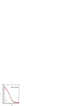
Figure 1: (a): The epidemic threshold $\lambda_{c}$ versus $\alpha$ with the exponent $\beta=0$ in BA networks. (b): The epidemic threshold $\lambda_{c}$ versus $\beta$ with the exponent $\alpha=1.0$ in BA networks.

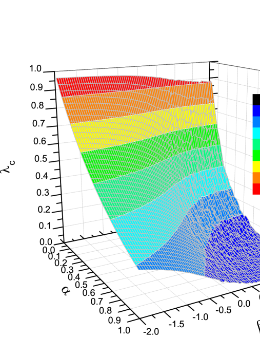
Figure 2: The epidemic threshold $\lambda_{c}$ in a 3D-graph, which is made up with various $\alpha$ and $\beta$ in BA networks.

In order to get a intuitionistic relation with $\lambda_{c}$, $\alpha$ and $\beta$, we have performed numerical simulations for the epidemic threshold. Firstly, on the basis of the simulated stochastic realizations of SIR model on BA networks [9] of which the theoretical scale-free exponent is 3 ($\gamma=3$), we fix $\beta=0$ and adjust $\alpha$ between 0 and 1 to show the transformation of epidemic threshold $\lambda_{c}$. In this case the critical value of $\alpha$ is: $\alpha_{c}=\gamma-\beta-2=1$, below which $\lambda_{c}$ is a nonzero finite value. As figure 1(a) displays, the value of $\lambda_{c}$ is greater than 0.01 with the relation $\alpha\ll 1$, vice versa. Secondly, we fix $\alpha=1.0$ and adjust $\beta$ between -2 and 2 to show the transformation of $\lambda_{c}$. In this case the critical value of $\beta$ is: $\beta_{c}=\gamma-\alpha-2=0$, below which $\lambda_{c}$ is a nonzero finite value. As figure 1(b) displays, at the point of $\beta_{c}=0$, $\lambda_{c}\simeq 0.03$, and $\lambda_{c}$ will take on a much faster change in $\beta<0$ than the one in $\beta>0$, and the finiteness of $\lambda_{c}$ is apparent when $\beta<-0.5$. From figure 1, one can see the simulations are consistent with the analytic results about critical threshold when we consider the effect of finite scale of the substrate work we use. Moreover, it is observed that the decreasing trend of $\lambda_{c}$ with increasing $\alpha$ is much quicker than the one with increasing $\beta$, that is to say, $\alpha$ is more sensitive than $\beta$ in the transformation of epidemic threshold $\lambda_{c}$, which means $\alpha$ is the leading factor for the transformation of $\lambda_{c}$ in the present model. Figure 2 displays the epidemic threshold in a 3D-graph, which is made up with various $\alpha$ and $\beta$, and the critical condition for a nonzero finite threshold is $\alpha+\beta<1$. One can see that $\lambda_{c}$ is small in the blue area where the great mass of data meet the condition that $\alpha+\beta>1$, which is the condition of threshold vanishing.

3.3 Propagation behavior

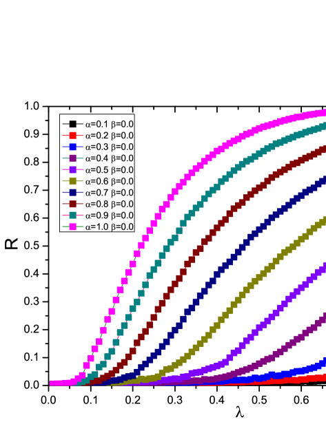
Figure 3: The steady epidemic prevalence $R$ versus $\lambda$ for SIR model in BA networks with $N=10^{4}$, $\langle k\rangle=6$, $\beta=0$, and $\alpha$=1.0, 0.9, 0.8, $\cdots$, 0.2, 0.1 (from top to bottom).

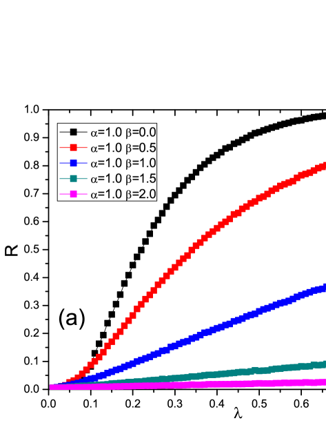
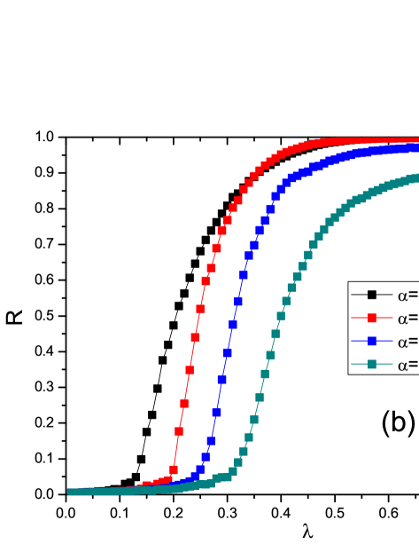
Figure 4: The steady epidemic prevalence $R$ versus $\lambda$ for SIR model in BA networks with $N=10^{4}$, $\langle k\rangle=6$, $\alpha=1.0$, and (a): $\beta$=0, 0.5, 1.0, 1.5, 2.0 (from top to bottom); (b): $\beta$=-0.5, -1.0, -1.5, -2.0 (from top to bottom).

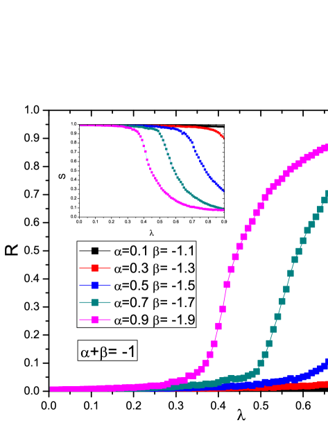
Figure 5: The steady epidemic prevalence $R$ versus $\lambda$ for SIR model in BA networks with $N=10^{4}$, $\langle k\rangle=6$, $\alpha+\beta=-1$, and from top to bottom: $\alpha$=0.9, 0.7, 0.5, 0.3, 0.1; accordingly $\beta$=-1.9, -1.7, -1.5, -1.3, -1.1. The inset shows the susceptible density $S$ versus $\lambda$ with the same combination of $\alpha$ and $\beta$.

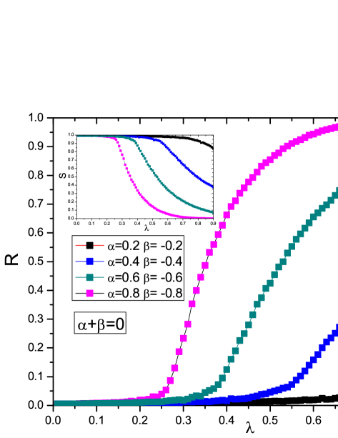
Figure 6: The steady epidemic prevalence $R$ versus $\lambda$ for SIR model in BA networks with $N=10^{4}$, $\langle k\rangle=6$, $\alpha+\beta=0$, and from top to bottom: $\alpha$=0.8, 0.6, 0.4, 0.2; accordingly $\beta$=-0.8, -0.6, -0.4, -0.2. The inset shows the susceptible density $S$ versus $\lambda$ with the same combination of $\alpha$ and $\beta$.

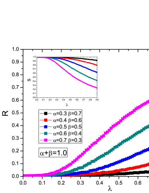
Figure 7: The steady epidemic prevalence $R$ versus $\lambda$ for SIR model in BA networks with $N=10^{4}$, $\langle k\rangle=6$, $\alpha+\beta=1$, and from top to bottom: $\alpha$=0.7, 0.6, 0.5, 0.4, 0.3; accordingly $\beta$=0.3, 0.4, 0.5, 0.6, 0.7. The inset shows the susceptible density $S$ versus $\lambda$ with the same combination of $\alpha$ and $\beta$.

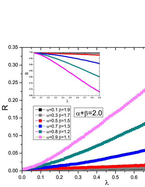
Figure 8: The steady epidemic prevalence $R$ versus $\lambda$ for SIR model in BA networks with $N=10^{4}$, $\langle k\rangle=6$, $\alpha+\beta=2$, and from top to bottom: $\alpha$=0.9, 0.8, 0.7, 0.5, 0.3, 0.1; accordingly $\beta$=1.1, 1.2, 1.3, 1.5, 1.7, 1.9. The inset shows the susceptible density $S$ versus $\lambda$ with the same combination of $\alpha$ and $\beta$.

For further investigation of the epidemic dynamics of the present model, we study the propagation behavior of the epidemic spreading. Firstly, we investigate the average epidemic prevalence in the steady stage of epidemic evolution with different combinations of $\alpha$ and $\beta$. From the analysis in section 3, it is easily to conclude that $I_{k}=0$ at the epidemic critical point of $\lambda$, which will induce a quite small $R_{k}$, and we can approximately get $\phi\simeq 0$ according to the relationship $\phi=\sum_{k}k^{\alpha}P(k)R_{k}$. Then, expanding the rhs of equation (14) for the small $\phi$, and ignoring the higher-order terms, we obtain

$$\frac{\langle k^{\alpha+\beta+1}\rangle}{\langle k^{\beta+1}\rangle}\lambda-\frac{1}{2}\frac{\langle\alpha+2\beta+2\rangle}{\langle k^{1+\beta}\rangle^{2}}\lambda^{2}\phi=1.$$ (20)

Next, we compute the derivative of equation (20) for $\lambda$ at the critical point, as follows:

$$\frac{d\phi}{d\lambda}|_{\lambda_{c}}=\frac{2\langle k^{\alpha+\beta+1}\rangle^{3}}{\langle k^{1+\beta}\rangle\langle k^{\alpha+2\beta+2}\rangle}.$$ (21)

As referred above, one can obtain that

$$R=\sum_{k}P(k)R_{k}=1-\sum_{k}P(k)e^{-\lambda k^{1+\beta}\phi/\langle k^{1+\beta}\rangle},$$ (22)

consequently,

$$\frac{dR}{d\lambda}|\lambda_{c} = \sum_{k}P(k)\lambda_{c}\frac{k^{1+\beta}}{\langle k^{1+\beta}\rangle}\frac{d\phi}{d\lambda}|\lambda_{c}$$ (23)

$$= \frac{2\langle k^{\alpha+\beta+1}\rangle^{2}}{\langle k^{\alpha+2\beta+2}\rangle}.$$

Similarly, in the considering of general scale-free networks as referred above, equation (23) can be written as follows:

$$\frac{dR}{d\lambda}|\lambda_{c} = \frac{2c(\alpha+2\beta+3-\gamma)}{(\alpha+\beta+2-\gamma)^{2}}\frac{(k_{\rm max}^{\alpha+\beta+2-\gamma}-k_{\rm min}^{\alpha+\beta+2-\gamma})^{2}}{k_{\rm max}^{\alpha+2\beta+3-\gamma}-k_{\rm min}^{\alpha+2\beta+3-\gamma}}\propto k_{\rm max}^{\alpha+1-\gamma}.$$ (24)

The obtained results shows, the exponent $\alpha$ will make a primary contribution to the velocity of increasing of the steady epidemic prevalence ($R$) by given the topology of a underlying network. Combining the analysis in section 3, for a fixed sum of $\alpha$ and $\beta$, one can conclude that the more ratio of $\alpha$ to $\beta$ is , the larger the $\lambda_{c}$ is, and the slowly the $R$ grows as $\lambda$ increases (since the most large-scale real networks have the relationship $\alpha+1-\gamma<0$).

For a better understanding of the epidemic propagation behavior, we take numerical simulations with various combination of $\alpha$ and $\beta$ on BA networks ($\gamma=3$). Firstly, we investigate the impact of $\alpha$ and $\beta$ separately, which are the two particular cases: $\alpha=1.0$ with different $\beta$, and $\beta=0$ with different $\alpha$. Figure 3 displays the effects of $\alpha$ on the steady epidemic prevalence $R$ with $\beta=0$. As the figure shows, for a same $\lambda$, one can observe the slope of $R$ grows as $\alpha$ increases (see $\alpha$=0.9, 0.8, $\cdots$, 0.2, 0.1), which is consistent with the analytical results from equation (24). Figure 4 displays $R$ versus $\lambda$ in the case of $\alpha=1.0$, and figure 4(a): $\beta$=0, 0.5, 1.0, 1.5, 2.5 (from top to bottom); figure 4(b): $\beta$=-0.5, -1.0, -1.5, -2.5 (from top to bottom). As shown in figure 4, the larger the absolute value of $\beta$ is, the more slowly the $R$ grows. On the other hand, for a general case ($\alpha\neq 1$ and $\beta\neq 0$), according to the critical equation $\alpha+\beta+2=\gamma$ and the algebraic sign of the sum $\alpha+\beta$, we consider four representative combinations of $\alpha$ and $\beta$, which are $\alpha+\beta=-1$, $\alpha+\beta=0$, $\alpha+\beta=1$ and $\alpha+\beta=2$. In each combination, there also has been divided into several different configurations by the ratio of $\alpha$ to $\beta$. As shown in figures (5 - 8), for a fixed sum of $\alpha$ and $\beta$, one can see the $R$ grows more quickly as the ratio increasing, which is consistent with our analytical results that $\alpha$ is a more sensitive factor to $R$. And further more, since $\alpha+\beta>1$, one can see the epidemic threshold $\lambda_{c}$ is quite small (tends to zero, considering the effects of finite size) in figure 4(a) and figure 8, which is also consistent with the critical condition of $\lambda_{c}$; otherwise, for $\alpha+\beta<1$, $\lambda_{c}$ becomes to be a nonzero finite value as shown in figure 3, figure 4(b), figure 5 and figure 6. For the early stage of $\lambda>\lambda_{c}$ in figures (3 - 8), one can see the $R$ grows in an exponential form with $\lambda$ increases, then the growth rate will take off slowly for $\lambda\gg\lambda_{c}$, at last, it will tend to be zero, which means the value of $R$ have attained a steady value.

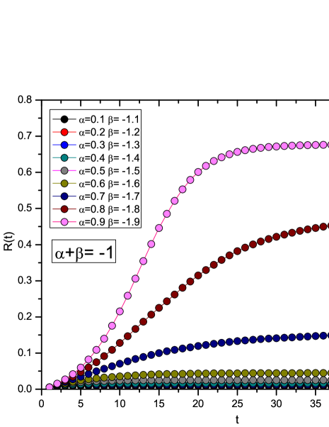
Figure 9: The temporal epidemic prevalence $R(t)$ versus $\lambda$ for SIR model in BA networks with $N=10^{4}$, $\langle k\rangle=6$, $\alpha+\beta=-1$, and from top to bottom: $\alpha$=0.9, 0.8, 0.7, $\cdots$, 0.2, 0.1; accordingly $\beta$=-1.9, -1.8, -1.7, $\cdots$, -1.2, -1.1.

Figure 10: The temporal epidemic prevalence $R(t)$ versus $\lambda$ for SIR model in BA networks with $N=10^{4}$, $\langle k\rangle=6$, $\alpha+\beta=0$, and from top to bottom: $\alpha$=0.8, 0.7, $\cdots$, 0.2, 0.1; accordingly $\beta$=-0.8, -0.7, $\cdots$, -0.2, -0.1.

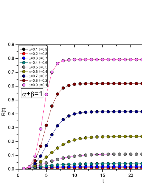
Figure 11: The temporal epidemic prevalence $R(t)$ versus $\lambda$ for SIR model in BA networks with $N=10^{4}$, $\langle k\rangle=6$, $\alpha+\beta=1$, and from top to bottom: $\alpha$=0.9, 0.8, 0.7, $\cdots$, 0.2, 0.1; accordingly $\beta$=0.1, 0.2, 0.3, $\cdots$, 0.8, 0.9.

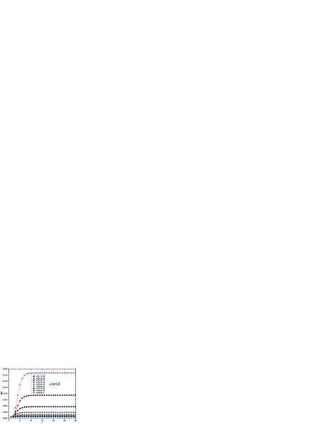
Figure 12: The temporal epidemic prevalence $R(t)$ versus $\lambda$ for SIR model in BA networks with $N=10^{4}$, $\langle k\rangle=6$, $\alpha+\beta=2$, and from top to bottom: $\alpha$=0.9, 0.8, 0.7, $\cdots$, 0.2, 0.1; accordingly $\beta$=1.1, 1.2, 1.3, $\cdots$, 1.8, 1.9.

For investigating the temporal propagation behavior, we simulate the time behavior of $R(t)$ for SIR model on BA networks with $\lambda=0.5$. As displayed in figure 9 ($\alpha+\beta=-1$), figure 10 ($\alpha+\beta=0$), figure 11 ($\alpha+\beta=1$) and figure 12 ($\alpha+\beta=2$), one can see that, the prevalence $R(t)$ grows in an exponential form in the early stage, and then stabilizes in a nonzero value as time goes on. Since $\lambda$ may be smaller than $\lambda_{c}$ when the value of $\alpha$ is much small such as $\alpha=0.1,0.2$, thus if $\lambda<\lambda_{c}$, the steady value of $R(t)$ (i.e., $R$) will be quite small, which approximatively equals to the initial density of infected nodes; when $\lambda>\lambda_{c}$, the prevalence $R(t)$ is higher as the ratio of $\alpha$ to $\beta$ gets larger at the same time of $t$, as the figures display. Moreover, it is observed that the steady value of $R(t)$ is smaller in figure 12 compared with the other figures (9 - 11). Although the exact solution of $R(t)$ about $\alpha$ and $\beta$ which can demonstrate the difference well is difficult to be managed here, from a qualitative perspective, we believe that’s because of the trait of SIR model. In figure 12, $\alpha+\beta=2$ which will induce a small threshold $\lambda_{c}$, thus at the early stage of evolution many susceptible nodes will be infected in view of the relation of $\lambda\gg\lambda_{c}$, and due to the immune rate we set is unity ($\mu=1$), the old infected nodes will become removed ones that cant’t be infected any more at the same time. Consequently the optional objects for a infected node will decrease as time evolutes, Moreover, there will be many infected nodes surrounded by the removed ones. Under this situation, the epidemic spreading will arrive at a equilibrium much more quickly, and thus the epidemic prevalence in the steady stage also will be a small value as figure 12 displays.

4 Conclusion and discussion

To sum up, in this paper, we have investigated the dynamical behavior of SIR model with weighted transmission rate and nonlinear infectivity, we present that one can adjust the exponent $\alpha$ and $\beta$ to control the epidemic threshold which is absent for the standard SIR model in scale-free networks. The critical value just depends on the exponent $\alpha$ and $\beta$ for a given topology of networks (a fixed value of $\gamma$), and $\alpha$ is more sensitive than $\beta$ for the transformation of the epidemic threshold and epidemic prevalence, which agrees with the numerical simulations very well. And the numerical results of the time behavior of $R(t)$ also have been presented, where the remarkable result is that, for a fixed $\lambda$, the smaller threshold $\lambda_{c}$ will induce a smaller epidemic prevalence at the equilibrium.

In a way, epidemic spreading can be managed as a reaction-diffusion process [40, 41, 42], which also has a very close relation with information retrieval, peer-trust and influence spreading. The efficient diffusion or inefficient diffusion maybe has its merits in various natural and artificial networks. Our work might deliver some useful information or new insights in designing data layout, city layout and network layout for performing their best advantages.

References

References

- [1] Kermack W O and McKendrick A G 1927 Proc. R. Soc. London. Ser. A 115 700
- [2] Bailey and N T J 1975 The Mathematical Theory of Infectious Diseases, second ed (London: Griffin)
- [3] Anderson, May and R M 1992 Infectious Disease in Humans (Oxford: Oxford University Press)
- [4] Albert R and Barabsi A-L 2002 Rev. Mod. Phys. 74 47
- [5] Amaral L A N, Scala A, Barthlemy M and Stanley H E 2000 Proc. Natl. Acad. Sci. USA. 97 1149
- [6] Dorogovtsev S N and Mends J F F 2003 Evolution of Networks: From Biological Nets to the Internet and WWW (Oxford: Oxford University Press)
- [7] Pastor-Satorras R and Vespignani A 2004 Evolution and Structures of the Internet: A Statistical Physics Approach (Cambridge: Cambridge University Press)
- [8] Watts D J and Strogats S H 1998 Nature 393 440
- [9] Barabsi A-L and Albert R 1999 Science 286 509
- [10] Faloutsos M, Faloutsos P and Faloutsos C 1999 Comput. Commm. Rev. 29 251
- [11] Albert R, Jeong H, Barabsi A-L 1999 Nature 401 130
- [12] Cohen R, Erez K, ben-Avraham D and Havlin S 2000 Phys. Rev. Lett. 85 4626
- [13] Newman M E J 2001 Phys. Rev. E 64 016132
- [14] Strogatz S H 2001 Nature 410 268
- [15] Newman M E J 2003 SIAM Rev. 45 167
- [16] Boccaletti S, Latora V, Moreno Y, Chavez M and Hwang D-U 2006 Phys. Rep. 424 175
- [17] Daily, D J, Gani and J 2001 Epodemic Modelling: An Introduction (Cambridge: Cambridge University Press)
- [18] Diekmann, O, Heesterbeek and J A P 2000 Mathematical Epidemiology of Infectious Disease: Model Buliding, Analysis and Interpretation (New York: Wiley)
- [19] Barthlemy M, Barrat A, Pastor-Satorras R and Vespihnani A 2004 Phys. Rev. Lett. 92 178701
- [20] Barthlemy M, Barrat A, Pastor-Satorras R and Vespihnani A 2005 J. Theor. Biol. 235 275
- [21] Pators-Satorras R and Vespignani A 2001 Phys. Rev. Lett. 86 3200
- [22] Pators-Satorras R and Vespignani A 2001 Phys. Rev. E 63 066117
- [23] Bogu M and Pators-Satorras R 2002 Phys. Rev. E 66 047104
- [24] Bogu M, Pators-Satorras R and Vespignani A 2003 Phys. Rev. Lett. 90 028701
- [25] Yan G, Fu Z Q and Chen G 2008 Eur. Phys. J. B 26 370
- [26] May R M and Lloyd A L 2002 Phys. Rev. E 64 066112
- [27] Lloyd A L and May R M 2001 Science 292 1316
- [28] Moreno Y, Pators-Satorras R and Vespignani A 2002 Eur. Phys. J. B 26 521
- [29] Moreno Y, Gomez J B and Pacheco A F 2003 Phys. Rev. E 68 035103
- [30] Joo J and Lebowitz J L 2004 Phys. Rev. E 69 066105
- [31] Olinky R and Stone L 2004 Phys. Rev. E 70 030902
- [32] Pators-Satorras R and Vespignani A 2002 Handbok of Graphs and Networks: From the Genome to the Internet (Berlin: Wiley-VCH)
- [33] Barrat A, Barthlemy M, Pators-Satorras R and Vespignani A 2004 Proc. Natl. Acad. Sci. USA 101 3747
- [34] Barrat A, Barthlemy M and Vespignani A 2004 Phys. Rev. Lett. 92 228701
- [35] Barrat A, Barthlemy M and Vespignani A 2004 Phys. Rev. E 70 066149
- [36] Macdonald P J, Almaas E and Barabsi A-L 2005 Europhys. Lett. 72 10232
- [37] Newman M E J 2002 Phys. Rev. Lett. 89 208701
- [38] Zhou T, Liu J G, Bai W L, Chen G R and Wang B H 2006 Phys. Rev. E 74 056109
- [39] Fu X, Samll M, Walker D M and Zhang H 2008 Phys. Rev. E 77 036113
- [40] Gallos L K and Argyrakis P 2005 Phys. Rev. E 72 017101
- [41] Baronchelli A, Catanzaro M and Pastor-Satorras R 2008 Phys. Rev. E 78 016111
- [42] Colizza V, Pastor-Satorras R and Vespignani A 2007 Nat. Phys. 3 276