Considerations on the magnitude distributions of the Kuiper belt and of the Jupiter Trojans

Abstract

By examining the absolute magnitude ($H$) distributions (hereafter HD) of the cold and hot populations in the Kuiper belt and of the Trojans of Jupiter, we find evidence that the Trojans have been captured from the outer part of the primordial trans-Neptunian planetesimal disk. We develop a sketch model of the HDs in the inner and outer parts of the disk that is consistent with the observed distributions and with the dynamical evolution scenario known as the ‘Nice model’. This leads us to predict that the HD of hot population should have the same slope of the HD of the cold population for $6.5<H<9$, both as steep as the slope of the Trojans’ HD. Current data partially support this prediction, but future observations are needed to clarify this issue. Because the HD of the Trojans rolls over at $H\sim 9$ to a collisional equilibrium slope that should have been acquired when the Trojans were still embedded in the primordial trans-Neptunian disk, our model implies that the same roll-over should characterize the HDs of the Kuiper belt populations, in agreement with the results of Bernstein et al. (2004) and Fuentes and Holman (2008). Finally, we show that the constraint on the total mass of the primordial trans-Neptunian disk imposed by the Nice model implies that it is unlikely that the cold population formed beyond 35 AU.

1 Introduction

Models have recently proposed that the Jovian Trojan asteroids and the Kuiper belt objects share a common origin — they formed in a massive primordial disk that stretched from roughly 15 to $\sim\!30\,$AU and were transported to their current locations during the phase of orbital migration of the giant planets (Morbidelli et al. 2005; Levison et al. 2008). This connection is a main result of the so-called Nice model (Tsiganis et al., 2005; Gomes et al., 2005). In the Nice model, the giant planets are assumed to have formed in a compact configuration (all were located between 5–$15\,$AU) and be surrounded by a $\sim\!35M_{\oplus}$ planetesimal disk that extended to about $30\,$AU. It introduced the idea that Jupiter and Saturn were so close in the past that they had to migrate across their mutual 1:2 resonance. This led to a violent, but temporary phase of instability in the dynamics of the four outer planets. The gravitational interaction between the ice giants and the planetesimals damped the orbits of these planets - leading them to evolve onto their current orbits.

As a result, however, $\sim\!35M_{\oplus}$ of planetesimals were scattered throughout the Solar System. Some were then captured into stable orbits by the migrating planets. In particular, as Jupiter and Saturn passed through various resonances with one another, a small number of planetesimals would have been captured into the Trojans regions of Jupiter. Morbidelli et al. (2005) showed that this process quantitatively reproduces both the number and the orbital element distribution of the observed Trojan swarms. Another example can be found in the trans-Neptunian region, which, according to Levison et al. (2008; L08 hereafter), was populated during the high-eccentricity phase of Neptune. The simulations in L08 are the most successful to date at reproducing the observed characteristics of the Kuiper belt.

If the above argument is correct, then there should be a genetic link between the Trojan asteroids of Jupiter and the Kuiper belt objects (hereafter KBOs), which should be detectable by studying their physical characteristics. Perhaps the most significant physical property of a population is its size-distribution, or equivalently, for a size-independent albedo, its absolute magnitude ($H$) distribution (hereafter HD). In particular, if the Trojan and Kuiper belt populations are related they should have similar HDs. This assumes that they have not undergone significant collisional evolution since they were emplaced in their current orbits. Levison et al. (2008b) has shown that this is a reasonable assumption for the Trojans. The fact that, as we show below, the HDs of the Trojans and the Kuiper belt are consistent with one another argues that this is a reasonable assumption for the Kuiper belt as well — at least at the sizes we are concerned with here. Thus, the goal of this paper is to study the HDs of the Trojans and the Kuiper belt to search for any genetic link.

Before we proceed, however, we need to discuss the structure of the Kuiper belt in more detail. The Kuiper belt has very intriguing properties that show that the primordial disk of trans-Neptunian planetesimals was drastically sculpted by a variety of dynamical processes. A characteristic of particular relevance here is the co-existence of cold and hot populations (defined by having inclination respectively smaller and larger than 4.5 degrees; Brown, 2001) with different physical properties (Levison and Stern, 2001; Tegler and Romanishin, 2000, 2003; Doressoundiram et al., 2001, 2005; Trujillo and Brown, 2002; Bernstein et al., 2004, B04 hereafter; Elliot et al., 2005; see however Pexinho et al., 2008 for a proposed alternative inclination divide between populations of different color properties). Levison and Stern (2001) showed that all of the largest KBOs are found in the hot population. This led them to suggest that the hot population formed closer to the Sun (where large objects would form more quickly) than the cold population, and were transported outward as the orbits of the planets evolved (see Gomes, 2003). The difference in the size-distributions was confirmed by B04, who showed that the HD for the hot population is shallower at the bright end than that of the cold.

L08 explained the differences between the hot and cold populations in the context of the Nice model by showing that the cold population is derived almost exclusively from the outer part of the disk, while the hot population samples the full disk more evenly. Thus they concluded that the different HDs of the cold and the hot populations at the bright end can be explained if the HD was not uniform throughout the original planetesimal disk; instead, the outer part of the disk had a steep HD and the inner part had a shallow HD and contained the largest objects.

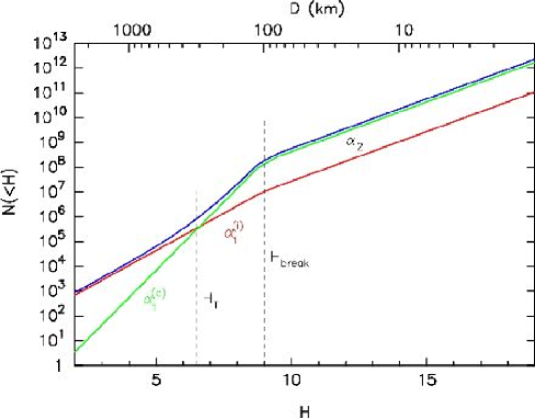
Figure 1: Sketch of the HDs in the inner (red) and outer (green) parts of the disk, showing the meaning of the quantities $\alpha_{1}^{(i)}$, $\alpha_{1}^{(o)}$, $\alpha_{2}$, $H_{T}$ and $H_{\rm break}$. The values of these quantities that we adopt to draw this figure are those that characterize the disk model defined in Sect. 3. The blue curve shows the HD obtained summing the HDs for the inner and the outer parts of the disk. We expect that the current HDs of the cold and of the hot populations of the Kuiper belt have the same shapes of the green and of the blue curves, respectively. The HD of the Trojans has the shape of the blue curve, but is defined only for $H>7.5$ (the absolute magnitude of the brightest Trojan). The correspondence between the size scale (top) and $H$ scale (bottom) has been obtained assuming a 4.5% albedo. For simplicity, we assume that the albedo is size-independent.

Studies of the collisional accretion and erosion of planetesimals (e.g. Kenyon and Bromley, 2004) show that a small-body population should have a cumulative size distribution that can be exemplified by a broken power-law: the exponent $q_{1}$ of this power-law for large sizes is a characteristic of the accretion process and thus it can have different values for different populations; the exponent $q_{2}$ for small sizes is instead quite universal and characteristic of collisional equilibrium (i.e. $q_{2}\sim-2$). The roll-over of the power-law from exponent $q_{1}$ to exponent $q_{2}$ occurs around a size $R_{\rm break}$ which can also differ from one population to another. Remember now that, if the albedo is size-independent, a cumulative power-law size distribution with exponent $q$ is equivalent to an exponential HD of type $N(<H)\propto 10^{\alpha H}$, with $\alpha=-q/5$. Thus, it is reasonable to expect that the inner and outer parts of the original trans-Neptunian disk each followed a broken HD, with their own values of $\alpha_{1}$ at the bright end ($\alpha_{1}^{(i)}$ for the inner disk, $\alpha_{1}^{(o)}$ for the outer disk, with $\alpha_{1}^{(i)}<\alpha_{1}^{(o)}$) and rolling over to $\alpha_{2}\sim 0.4$ at some $H\sim H_{\rm break}$. These broken HDs with different $\alpha$-slopes can be visualized in Fig. 1.

The Nice model implies that the HD of the Trojans, hot Kuiper belt, and cold Kuiper belt populations should each be a combination of the HDs found in the inner and outer parts of the original planetesimal disk. In practice, in each magnitude range, these populations should have inherited the HD of the part of the disk from which they captured most of the objects. Thus we expect that the currently observed Trojans and Kuiper belt populations have HDs with three exponents: the brightest objects ($H<H_{T}$) should have $\alpha=\alpha_{1}^{(i)}$; the intermediate objects ($H_{T}<H<H_{\rm break}$) should have $\alpha=\alpha_{1}^{(o)}$; the faint end ($H>H_{\rm break}$) should have $\alpha=\alpha_{2}$. The absolute magnitude at the transition between the first two exponents, $H_{T}$, is a function of the mixing ratio of the inner and outer disk in each population and therefore could change from one population to another. In our analysis below, we assume this simple HD as a template for analyzing the various populations of interest.

2 Absolute magnitude distributions of multi-opposition objects

We have considered the list of multi-opposition trans-Neptunian objects given by the Minor Planet Center (see http://www.cfa.harvard.edu/iau/lists/TNOs.html) as of April 14, 2008. This list excludes the so-called Scattered disk objects (Duncan and Levison, 1997; Luu et al., 1997). We have selected the bodies with $40<a<47.4$ AU, in order to exclude those in the 2:3 and 1:2 resonances with Neptune, to simplify the discussion. Of the selected objects, those with $i<4.5^{\circ}$ have been classified in the cold population, and the remainder in the hot population, in agreement with previous studies (Brown, 2001; Trujillo and Brown, 2002; Elliot et al., 2005).

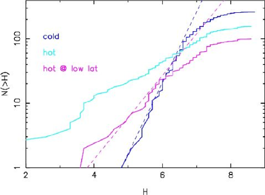
Figure 2: The absolute magnitude ($H$) cumulative distributions of the cold population (blue), of the hot population (cyan) and of the objects of the hot population discovered within $4.5^{\circ}$ of the ecliptic (magenta). For reference, the thin dashed blue line has a slope of $1.1$; the thin dashed magenta line has a slope of $0.65$.

Fig. 2 shows the cumulative HDs in the cold (solid blue curve) and hot (solid cyan curve) populations. It is evident that the HD in the hot population appears to be much shallower. This, however, could be due to a bias, because part of the hot population has been discovered in wide field surveys with shallower limiting magnitudes that strayed farther from the ecliptic than the deep surveys that discovered the smaller cold population objects. Thus, in Fig. 2, we also plot the HD of the hot population objects discovered within $4.5^{\circ}$ (solid purple curve) from the ecliptic. In doing this, we believe that, although we have not removed all observational selection effects, we have chosen our objects so that the hot and cold population suffer from similar biases. Thus, we believe that any difference that we see in the distributions are real. Still, the hot HD appears shallower than that of the cold population. As we explained above, this result is not new (Levison and Stern 2001; B04).

In Fig. 2 the observed low-$H$ end (i.e. large sizes) of the HD of the cold population is fit with a line of slope $\alpha=1.1$ (dashed blue line). This slope is somewhat shallower than the preferred slope ($1.3$) of B04, but falls within its 1-$\sigma$ uncertainty (which extends down to $\alpha\sim 1$). In addition, we find that a line with the best fit slope of the debiased hot population in B04 (i.e. $\alpha=0.65$, dashed purple line) matches the observed HD of the low-latitude hot population reasonably well. This general agreement with B04 argues that the slopes of the observed low-latitude HDs that we determined with our simple techniques from the MPC catalogue do not suffer from significant observational biases. Thus, we feel comfortable comparing our results directly to the Trojans.

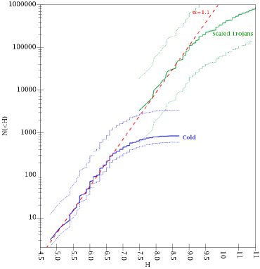
Figure 3: The cumulative $H$-distributions of the cold population (blue lines) and of the Trojan population (green lines). The blue dotted lines bracket the current number of cold KBOs according to B04. The dotted green curves show the current HD of the Trojans, scaled by factors of 600 (lower curve) and 19,000 (upper curve), which correspond to the minimal and maximal ratios between the populations of cold KBOs and Trojans, according to the Nice model. The solid blue and green curves show the observed HDs of the cold KBOs and Trojans, scaled by appropriate factors so that they fall within the boundaries provided by the dotted curves. The red dashed line corresponds to an HD with $\alpha=1.1$. This line highlights that the HD of the Trojan population with $H<9$ has the same slope of the HD of the cold population with $H<6.5$. We interpret the apparent turn-over of the HD of the cold population at $H=6.5$ as due to observational biases. The common slope of the HDs of cold KBOs and Trojans supports the genetic link between these two populations predicted by the Nice model.

As a first step in our analysis, we compare the HDs of the cold population with that of the Trojans of Jupiter. In order to make this comparison, however, we need to scale the observed distributions in a physically meaningful way. Using the information in B04, we estimate that there should be between about 50 and 200 objects in the cold population with $H<6$. The dotted blue curves in Fig. 3 show the observed cold population scaled to these two extremes. To scale the Trojans, we make use of the fact that the Nice model predicts that both the cold Kuiper belt and the Trojans come from the primordial trans-Neptunian disk and provides the corresponding capture efficiencies. In particular, L08 showed that between 0.04% and 0.16% of the full original disk (inner plus outer parts) was captured in the cold Kuiper belt population during the migration of the planets. Morbidelli et al. (2005) calculated that the fraction of the full disk that was captured into the Trojans swarms with low libration amplitude orbits was between $0.85\times 10^{-7}$ and $0.65\times 10^{-6}$. Thus, we expect that the ratio of cold KBOs to Trojans should be between 600 and 19,000. The dotted green curves in the figure show the Trojan HD (which is complete to $H=11$; Szabó et al., 2007) scaled by these factors.

The solid blue and green curves in Fig. 3 show the observed HDs of the cold KB and the Trojans, respectively, scaled using factors that are consistent with the constraints discussed in the last paragraph. They illustrate that the two distributions have essentially the same slope at the bright end (we attribute the roll-off in the cold population for $H>H_{\rm bias}\sim 6.7$ to observational bias).

Of course, this close similarity between the slopes could be coincidental. We think, however, that this is unlikely, because this common slope is very steep and peculiar. Indeed, in the asteroid belt, no sub-population has a similar HD (with the possible exception of some super-catastrophic families). The cold population/Trojan slope is very far from a collisional equilibrium slope ($\alpha=$0.4–0.5; Dohnanyi, 1969). It is also steeper than what a prolonged phase of collisional coagulation would give (S. Kenyon, private communication). Thus, it would be odd that the Trojans and the cold population show the same slope if they were unrelated. Instead, we believe that their common HD slope is real and reveals the genetic link predicted by the Nice model (see sect. 1).

The Trojans’ HD shows a roll-over at $H_{\rm break}\sim 9$. Beyond this magnitude, the HD of the Trojans has a shallower slope with exponent $0.4$ (Jewitt et al., 2000; Szabó et al., 2007), consistent with the expected value of $\alpha_{2}$ (see sect. 1). Notice that the Trojan population is observationally complete down to absolute magnitude $H\sim 11$ (Szabó et al., 2007), so the observed roll-over of its HD is a real feature. Unfortunately, we do not know with certainty the Kuiper belt HDs at these magnitudes because of its greater distance. However, if the arguments in sect. 1 are correct, both the hot and cold populations Kuiper belt should show the same type of roll-over at these magnitudes. This is consistent with the results of B04 and Fuentes and Holman (2008).

We interpret the common slope of Trojans and cold KBOs as the slope of the HD of the outer part of the primordial trans-Neptunian disk (i.e. $\alpha_{1}^{(o)}=1.1$). The lack of a shallow part in the Trojans’ HD (i.e. with $\alpha\sim\alpha_{1}^{(i)}$) indicates that the $H_{T}$ for this population is brighter than the largest Trojan, i.e. $H_{T}\lesssim 7.5$. Similarly, the lack of a shallow part in the HD of the cold Kuiper belt suggests that this population must have $H_{T}\lesssim 4.8$.

We now turn to the hot population. As we described in sect. 1, we expect that there is a value of $H_{T}$, characteristic of this population, such that $\alpha=\alpha_{1}^{(i)}$ for $H<H_{T}$ and $\alpha=\alpha_{1}^{(o)}$ for $H_{T}<H<H_{\rm break}$. Because $\alpha_{1}^{(o)}$ is also the slope of the cold population, we expect that the HD of the hot population to steepen up so that its slope matches that of the cold population for objects fainter than $H_{T}$.

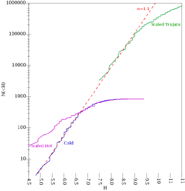
Figure 4: The same as Fig. 2, but only the solid curves for the cold KBOs and Trojans are plotted, while the HD of the hot population has been added, scaled up by a factor of 2.5. Notice that the observed HDs of the cold and of the hot populations are identical for $H>6.5$, in agreement with our predictions. See text for a broader discussion on this point.

In Fig. 4 we show the same green (scaled Trojan) and blue (cold KB) curves as were in Fig. 3, but we added the observed HD of the hot population discovered within $4.5^{\circ}$ of the ecliptic. We choose this subset of the hot population so that the observational biases are comparable for the two populations. To make the comparison more straightforward, we multiplied the hot population curve by a factor of 2.5. As one sees, the hot population HD is shallower for $H\lesssim 6.5$–7.0, but overlaps almost perfectly the HD of the cold population beyond this magnitude threshold. So, our prediction seems to be confirmed and $H_{T}$ for the hot population turns out to be $\sim 6.7$. This is not in conflict with Bernstein et al. (2004), who claimed that the the luminosity functions of the hot and cold populations have significantly different slopes for apparent magnitude $R\lesssim 23$ because, for an average distance of 42 AU, $R=23$ is equivalent to $H=6.7$.

A closer inspection of Fig. 4, however, reveals an important and troubling issue. Although the HDs of the hot and cold populations appear indistinguisheable for $H\gtrsim 6.7$, the HD of the hot population does not seem to become steeper, unlike what we would expect. Instead, it remains constant from $H\sim 6.0$ to $H\sim 7.5$. It is the HD of the cold population that becomes shallower to match that of the hot population! Above, we have argued that the reason for this apparent deviation of the cold population’s HD from the $\alpha=1.1$ line at $H\sim 6.7$ is that $H_{\rm bias}\sim 6.7$. If this is true, then Fig. 4 implies that $H_{T}\sim H_{\rm bias}$ and the bias conspires with the increase in the hot population’s $\alpha$ to produce a constant slope. This would be an amazing coincidence. To avoid this coincidence, the alternative interpretation is that $H_{\rm bias}\sim 7.5$ and that the HD of the hot belt has really a single slope up to at least $H_{\rm bias}$. This, though, would imply that the apparent roll-over of the HD of the cold population at $H\sim 6.7$ is also real (because biases change the slope only for $H>H_{\rm bias}\sim 7.5$). We see two problems with this alternative interpretation. First, it would seem another amazing coincidence that, whatever physical process caused this roll-over , it gave to the cold population exactly the same slope that the hot population has at larger sizes. Second, a roll-over at $H\sim 6.5$ would be in conflict with the results of all surveys devoted to unveil the true slope of the Kuiper belt luminosity function (Gladman et al., 2001; B04; Petit et al., 2006; Fraser et al., 2008; Fuentes and Holman, 2008), which reported no roll-over up to at least $H\sim 8$–9. On the other hand, it is also true that no team has ever reported a steepening of the HD of the hot population, but there have never been dedicated pencil beam surveys off ecliptic, so this feature, extended only over a couple of magnitudes, might have passed un-noticed.

Thus, for the moment we prefer our original interpretation to its alternative, although we feel quite uncomfortable about the coincidence that it implies. However, this is a testable hypothesis. If the above argument is correct, we predict that the hot population’s HD becomes as steep as the common cold-population/Trojan slope ($\alpha\sim 1.1$) for $H$ in the $\sim$6.5-9 interval. These predictions can be checked in the future when more data are collected and observational biases are removed.

3 The mass of the trans-Neptunian disk

The Nice model requires that the original mass of the trans-Neptunian planetesimal disk was 35–50 $M_{\oplus}$ (Tsiganis et al., 2005; Gomes et al., 2005). It is not obvious, a priori, that this requirement is consistent, even at the order of magnitude level, with the size distributions that we can infer from the considerations reported in the previous section for the inner and the outer parts of the disk. Here we discuss this consistency check.

In section 2 we concluded that $H_{T}$ for the hot population is $\sim 6.5$. The simulations in L08 show that particles in the inner and outer parts of the disk have roughly the same probability of being captured in the hot population. So, the value of $H_{T}$ characterizing the hot population should have been also the one at which the HDs of the inner and the outer parts of the disk crossed-over (i.e. $N_{\rm inner}(<H_{T})=N_{\rm outer}(<H_{T})$; see Fig. 1).

We have also seen that the the cold population has 50-200 objects with $H=6$, which is equivalent to 175 to 700 objects with $H<H_{T}\equiv 6.5$, for $\alpha=1.1$. The fraction of the full trans-Neptunian disk captured in the cold population is 0.04%–0.16% (L08). Thus, there were between $10^{5}$ and $1.7\times 10^{6}$ objects with $H<H_{T}$ in the disk, half of which in the inner and in the outer parts. Assuming an albedo of 4.5%, $H=6.5$ corresponds to $D\sim 300$ km.

For the outer part of the disk, $\alpha_{1}^{(o)}=1.1$ implies that the exponent of the cumulative size distribution is $q_{1}=-5.5$. The size of the largest object in the outer disk is the value $D_{\rm max}$ such that $N(>D_{\rm max})$=1. Given $q_{1}$ and the estimated number range of 300 km objects obtained above, $D_{\rm max}$ is 2,100-3,500 km.

For the inner part of the disk, we assume that the size distribution is truncated at $D_{\rm max}=$2,500 km (Pluto-size) and $q_{1}=-3$ (i.e. $\alpha_{1}^{(i)}=0.6$, which is within the slope uncertainties for the hot population; see B04). Scaling again from the number of 300 km objects, this gives between $\sim$ 100 and 1,500 objects of size $D_{\rm max}$. This is consistent with the estimate (L08) that roughly 1,000 Pluto-size objects had to exist in the disk (Charnoz and Morbidelli, 2007) estimated this number to be $\sim 300$).

For both the inner and the outer disks we assume $H_{\rm break}=9$. Assuming again that the albedo is 4.5%, this corresponds to $D_{\rm break}=100$ km. For smaller objects, we assume $\alpha_{2}=0.4$ (i.e. $q_{2}=-2$) as for the Trojans.

Now we have all the ingredients to compute the total mass (we assume a bulk density of 1g/cm³). We find that the mass of the inner disk is between 1.5 and 23 Earth masses; the mass of the outer disk is between 9 and 130 Earth masses. The total mass of the full disk is between 10 and 150 Earth masses. The order of magnitude uncertainty on the total mass comes from the comparable uncertainty on the total number of objects, illustrated by the green curves in Fig. 3. Nevertheless, the fact that our estimate brackets the disk mass required in the dynamical simulations of Tsiganis et al. (2005) and Gomes et al. (2005) gives, once again, confidence on the gross consistency of that model.

The extremes of the mass estimate correspond to $N(D>300{\rm km})=10^{5}$ and $1.7\times 10^{6}$, respectively. The total mass scales almost linearly with $N(D>300{\rm km})$, so that a total mass of 35 Earth masses would imply $N(D>300{\rm km})\sim 4\times 10^{5}$. The HDs shown in Fig. 1 have been normalized to this value.

4 Cold population: local or implanted?

In the original version of the Nice model, the planetesimal disk is assumed to be truncated at $\sim 34$ AU (Tsiganis et al., 2005; Gomes et al., 2005). The Kuiper belt is therefore empty. The cold population is captured into the Kuiper belt from within 34 AU (L08).

However, Morbidelli et al. (2008) showed that, from a purely dynamical point of view, the Nice model is also consistent with the existence of a local, low mass Kuiper belt population, extended up to 44 AU. In fact, the resulting $(a,e)$ distribution of cold population objects would be indistinguishable from that in L08. In the case where the outer edge was initially at 44 AU, about 7% of the particles initially in the Kuiper belt ($a>40$ AU, $q>38$ AU) remained there, although on modified orbits. The others escaped to planet-crossing orbits during the large eccentricity phase of Neptune. Thus, a local population could be consistent with the Nice model provided that its total number of objects in the 40–44 AU interval was about 15 times the one currently present in the cold population.

Here we examine this possibility at the light of the considerations of the previous sections. In particular, we re-work our estimates assuming that the outer disk contained 15 times the current number of bodies with $D>300$ km in the cold population in the 40–44 AU interval (i.e. from 2,500 to 10,000 bodies) and show that this would imply a radial distribution of the disk’s surface density that is unlikely.

Our argument is the following. Given that the median initial semi major axis of the bodies trapped in the Trojan region is $\sim 26$ AU, we assume that this was the boundary between the inner and the outer parts of the disk. If the surface density of the disk had a radial profile as $1/r$, there would have been an equal number of objects per linear AU. In this case, as 2,500–10,000 bodies with $D>300$ km were spread over 4 AU (40–44 AU interval), the full outer disk (26–44 AU) would have contained 11,000–45,000 bodies. Assuming a $1/r^{2}$ surface density profile, the total number would increase to 14,000–55,000. Remember now that the total number of bodies larger than 300 km (or $H<6.5\equiv H_{T}$) should have been the same in the inner and in the outer parts of the disk (because of the very definition of $H_{T}$). As we have seen in the previous section, if this number had really been $\lesssim$ 50,000, the total mass of the full disk would have been $\lesssim 10M_{\oplus}$, too low for the dynamics of the Nice model. Moreover, the disk would have contained less than $5\times 10^{5}$ bodies larger than 200 km (assuming $q_{1}^{(o)}=-5.5$), too low to explain the capture of a few Trojans of this size given a capture probability lower than $6.5\times 10^{-7}$ (Morbidelli et al., 2005).

To have a total mass in the disk of $\sim 35$ Earth masses, the number of $D>300$ km bodies in each part of the disk should have been $\sim$ 200,000, as computed in the previous section. With 2,500–10,000 bodies in the 40–44 AU region, this could have been achieved only if the disk had a surface density profile of $r^{-\beta}$ with $\beta\sim 7$–11. This is much steeper than any radial profile ever proposed or inferred from observations of extra-solar disks.

Therefore we conclude that, in the framework of the Nice model, it is unlikely that the planetesimal disk extended into the Kuiper belt region. Thus, the cold population should have been implanted into the Kuiper belt from a smaller initial heliocentric distance.

5 Conclusions

In this paper, we have given a fresh look at the HDs of the Kuiper belt objects and of the Jovian Trojans. We have partitioned the Kuiper belt objects between 40 and 47 AU into a cold and a hot population, according to their orbital inclinations (Brown, 2001). We have confirmed that the HD of the hot population is shallower than that of the cold population (Fig. 2) for $H<6.5$ (B04), which supports models in which these two populations are derived from different regions of the primordial trans-Neptunian planetesimal disk.

We have found that the slope of the bright end of the Trojan population is very similar to that of the cold Kuiper belt population (Fig. 3). This, if not just a coincidence, suggests a genetic link between the two populations. Of all the models proposed so far on the history of the Kuiper belt, only the Nice model predicts such a link.

Thus, we have developed a sketch model of the HDs in the inner and the outer parts of the trans-Neptunian disk that is consistent with the aspects of the Nice model and explains the similarity of the HDs of the Trojans and of the cold population. This HD model has led us to predict that the HD of the hot population should steepen up, so that its slope matches that of the cold population for $H\gtrsim 6.5$. The current data seem to support this prediction because they show that the HDs of the hot and of the cold populations are identical beyond this magnitude threshold (Fig. 4). However, we pointed out that it is disturbing that the observed HD of the hot population has a straight slope up to $H\sim 7.5$, because this would imply that the steepening up of the real HD is perfectly counterbalanced by the observational biases. Thus, this issue remains to be settled with future observations.

Our HD model of the disk also implies that it is unlikely that the cold population formed in situ, but suggests that this population was implanted into the Kuiper belt from a smaller heliocentric distance.

Acknowledgments

This work was done while the first author was on sabbatical at SWRI. A.M. is therefore grateful to SWRI and CNRS for providing the opportunity of this long term visit and for their financial support.

References

• Bernstein, G. M., Trilling, D. E., Allen, R. L., Brown, M. E., Holman, M., Malhotra, R. 2004. The Size Distribution of Trans-Neptunian Bodies. Astronomical Journal 128, 1364-1390.

• Brown, M. E. 2001. The Inclination Distribution of the Kuiper Belt. Astronomical Journal 121, 2804-2814.

• Charnoz, S., Morbidelli, A. 2007. Coupling dynamical and collisional evolution of small bodies. II. Forming the Kuiper belt, the Scattered Disk and the Oort Cloud. Icarus 188, 468-480.

• Dohnanyi, J. W. 1969. Collisional models of asteroids and their debris. Journal of Geophysical Research 74, 2531-2554.

• Doressoundiram, A., Barucci, M. A., Romon, J., Veillet, C. 2001. Multicolor Photometry of Trans-neptunian Objects. Icarus 154, 277-286.

• Doressoundiram, A., Peixinho, N., Doucet, C., Mousis, O., Barucci, M. A., Petit, J. M., Veillet, C. 2005. The Meudon Multicolor Survey (2MS) of Centaurs and trans-neptunian objects: extended dataset and status on the correlations reported. Icarus 174, 90-104.

• Duncan, M. J., Levison, H. F. 1997. A scattered comet disk and the origin of Jupiter family comets. Science 276, 1670-1672.

• Elliot, J. L., and 10 colleagues 2005. The Deep Ecliptic Survey: A Search for Kuiper Belt Objects and Centaurs. II. Dynamical Classification, the Kuiper Belt Plane, and the Core Population. Astronomical Journal 129, 1117-1162.

• Fraser, W. C., Kavelaars, J. J., Holman, M. J., Pritchet, C. J., Gladman, B. J., Grav, T., Jones, R. L., Macwilliams, J., Petit, J.-M. 2008. The Kuiper belt luminosity function from $m_{R}=21$ to 26. Icarus 195, 827-843.

• Fuentes, C. I., Holman, M. J. 2008. a SUBARU Archival Search for Faint Trans-Neptunian Objects. Astronomical Journal 136, 83-97.

• Gladman, B., Kavelaars, J. J., Petit, J.-M., Morbidelli, A., Holman, M. J., Loredo, T. 2001. The Structure of the Kuiper Belt: Size Distribution and Radial Extent. Astronomical Journal 122, 1051-1066.

• Gomes, R. S. 2003. The origin of the Kuiper Belt high-inclination population. Icarus 161, 404-418.

• Gomes, R., Levison, H. F., Tsiganis, K., Morbidelli, A. 2005. Origin of the cataclysmic Late Heavy Bombardment period of the terrestrial planets. Nature 435, 466-469.

• Jewitt, D. C., Trujillo, C. A., Luu, J. X. 2000. Population and Size Distribution of Small Jovian Trojan Asteroids. Astronomical Journal 120, 1140-1147.

• Kenyon, S. J., Bromley, B. C. 2004. The Size Distribution of Kuiper Belt Objects. Astronomical Journal 128, 1916-1926.

• Levison, H. F., Stern, S. A. 2001. On the Size Dependence of the Inclination Distribution of the Main Kuiper Belt. Astronomical Journal 121, 1730-1735.

• Levison, H. F., Morbidelli, A., Vanlaerhoven, C., Gomes, R., Tsiganis, K. 2008. Origin of the structure of the Kuiper belt during a dynamical instability in the orbits of Uranus and Neptune. Icarus 196, 258-273.

• Levison, H. F., Bottke, W., Gounelle, M., Morbidelli, A., Nesvorny, D., Tsiganis, K. 2008b. Chaotic Capture of Planetesimals into Regular Regions of the Solar System. II: Embedding Comets in the Asteroid Belt. AAS/Division of Dynamical Astronomy Meeting 39, #12.05.

• Luu, J., Marsden, B. G., Jewitt, D., Trujillo, C. A., Hergenrother, C. W., Chen, J., Offutt, W. B. 1997. A New Dynamical Class in the Trans-Neptunian Solar System.. Nature 387, 573-575.

• Morbidelli, A., Levison, H. F., Tsiganis, K., Gomes, R. 2005. Chaotic capture of Jupiter’s Trojan asteroids in the early Solar System. Nature 435, 462-465.

• Morbidelli, A., Levison, H. F., Gomes, R. 2008. The Dynamical Structure of the Kuiper Belt and Its Primordial Origin. The Solar System Beyond Neptune 275-292.

• Peixinho, N., Lacerda, P., Jewitt, D. 2008. Color-Inclination Relation of the Classical Kuiper Belt Objects. Astronomical Journal 136, 1837-1845.

• Petit, J.-M., Holman, M. J., Gladman, B. J., Kavelaars, J. J., Scholl, H., Loredo, T. J. 2006. The Kuiper Belt luminosity function from $m_{R}=22$ to 25. Monthly Notices of the Royal Astronomical Society 365, 429-438.

• Szabó, G. M., Ivezić, Ž., Jurić, M., Lupton, R. 2007. The properties of Jovian Trojan asteroids listed in SDSS Moving Object Catalogue 3. Monthly Notices of the Royal Astronomical Society 377, 1393-1406.

• Tegler, S. C., Romanishin, W. 2000. Extremely red Kuiper-belt objects in near-circular orbits beyond 40 AU. Nature 407, 979-981.

• Tegler, S. C., Romanishin, W. 2003. Resolution of the Kuiper belt object color controversy: two distinct color populations. Icarus 161, 181-191.

• Trujillo, C. A., Brown, M. E. 2002. A Correlation between Inclination and Color in the Classical Kuiper Belt. Astrophysical Journal 566, L125-L128.

• Tsiganis, K., Gomes, R., Morbidelli, A., Levison, H. F. 2005. Origin of the orbital architecture of the giant planets of the Solar System. Nature 435, 459-461.